www.nat-hazards-earth-syst-sci.net/15/187/2015/ doi:10.5194/nhess-15-187-2015
© Author(s) 2015. CC Attribution 3.0 License.
Randomly distributed unit sources to enhance optimization
in tsunami waveform inversion
I. E. Mulia and T. Asano
Department of Ocean and Civil Engineering, Kagoshima University, Kagoshima, Japan Correspondence to: I. E. Mulia ([email protected], [email protected])
Received: 24 March 2014 – Published in Nat. Hazards Earth Syst. Sci. Discuss.: 22 May 2014 Revised: 16 December 2014 – Accepted: 20 December 2014 – Published: 30 January 2015
Abstract. In tsunami waveform inversion using the con-ventional Green’s function technique, an optimal solution is sometimes difficult to obtain because of various factors. This study proposes a new method to both optimize the determina-tion of the unknown parameters and introduce a global opti-mization method for tsunami waveform inversion. We utilize a genetic algorithm that further enhanced by a pattern search method to find an optimal distribution of unit source loca-tions prior to the inversion. Unlike the conventional method that characterized by equidistant unit sources, our method generates a random spatial distribution of unit sources inside the inverse region. This leads to a better approximation of the initial profile of a tsunami. The method has been tested us-ing an artificial tsunami source with real bathymetry data. Comparison results demonstrate that the proposed method has considerably outperformed the conventional one in terms of model accuracy.
1 Introduction
Direct observation of sea surface deformation after the oc-currence of an earthquake is still difficult to obtain; therefore, its estimation is often performed by consideration of relevant seismic information or the hydrodynamic response of the sea determined from recorded tsunami waveforms. Determina-tion of sea surface deformaDetermina-tion generated by earthquakes is crucial to the success of tsunami modeling. One of the most frequently used methods for determining sea surface defor-mation is to presume it from a fault model (Mansinha and Smylie, 1971; Okada, 1985). A more realistic approach was proposed by Satake (1987) who analyzed recorded wave-forms to infer earthquake source parameters or particularly,
coseismic slip, using the Green’s function technique. Even though the fault model is still required, the division of a fault into smaller sub-faults allows the slip to be estimated in a heterogeneous manner, which leads to better approximation of sea surface deformation. A simpler method was actually introduced earlier by Aida (1972) for which no prior assump-tion of a fault model was needed. This study is in line with that of Aida because we are more interested in estimating sea surface deformation than a slip on the fault plane. The mo-tivation behind this is that tsunami excitation can sometimes occur as a result of various factors that are independent of the associated seismic characteristics (Geist, 2002).
mea-sure, the search towards optimality is confined by the uni-form distance of unit sources used in the regular Green’s function.
Tsunami waveform inversion sometimes falls into an ill-posed problem, in which small errors in the observed wave-forms are exceptionally amplified in the solution. Therefore, both the uniqueness and the stability of solutions are some-times difficult to attain without appropriate treatments. The most frequently employed techniques to maintain a stable solution is to use a smoothing constraint (Gusman et al., 2010, 2013; Saito et al., 2010). Other than that, Koike et al. (2003) suggested reducing the unknown parameters using the wavelet base to guarantee the uniqueness of the solution. However, they found later that the selection of the wavelet base was not straightforward. Another effort to overcome the issue was discussed by Voronina (2011). The study promoted a method to control numerical stability for the ill-posed prob-lem in tsunami waveform inversion by means of singular value decomposition and r-solutions techniques. In this pa-per, we proposed a new approach to tackle the same problem by determining the optimal position or spatial distribution of unit sources located around the tsunami source or epicenter. A genetic algorithm (GA) as a global optimization method, combined with a pattern search (PS) method, is employed to search the mentioned positions prior to the inversion. As the selected positions are probably located in between the initial unit sources, interpolations are performed during the opti-mization. Therefore, the Green’s function evolves dynami-cally at each generation of the GA and PS iteration.
2 Inversion method
Generally, the characteristics of tsunami propagation in deep water are linear. According to Satake (1987), even in shal-low coastal areas, the first leading waves recorded at coastal tide gauges are still well simulated by the linear long wave model. Therefore, a typical linear non-dispersive shallow wa-ter equation is used in the forward modeling to compute time histories of sea surface elevation at the specified observation points:
∂V
∂t = −g∇η ∂η
∂t = −∇ · {(d+η)V}
, (1)
whereηis the water elevation of the tsunami,V(u, v)is the depth-averaged horizontal fluid velocity vector,d is the wa-ter depth, andgis gravitational acceleration. Equation (1) is completed with two types of boundary conditions, as follows: (
V·n=g cη
V·n=0
, (2)
wherec=√ghis the wave speed and nis the unit vector normal to the boundary. The upper and lower expression in Eq. (2) represent open and closed boundary respectively.
The Green’s functionGi(x, y, t )indicating the recorded
synthetic waveforms at a location(x, y)corresponding to the ith unit sources is then constructed. This tsunami Green’s function is derived from 2-D linear shallow water equa-tion, Eq. (1), solved using numerical method with specified bathymetry resolutions. The total sea surface fluctuations at (x, y, t )can be expressed as follows:
η (x, y, t )=
i=N
X
i=1
wiGi(x, y, t ) , (3)
wherewi is the weighting factor for each unit source or the
unknown parameters to be determined by the inversion and N is the number of the unit source. Equation (3) is devel-oped based on the assumption of linear superposition con-sidering the nonlinearity for tsunamis in ocean basins to be small, such that it can be neglected (Liu and Wang, 2008). In vector notation, Eq. (3) can be reformulated as follows:
η=wG. (4)
Based on the least squares method, the vector of the unknown parametersw can be acquired by solving the following in-verse equation:
w=GTG−1GTη. (5)
In this study, we assume that the generation of the initial pro-file of the tsunami occur instantaneously. Therefore, incorpo-rating the time variation or transient deformation of the water surface is unnecessary.
3 Global optimization method
The ultimate purpose of a global optimization method is to find the extreme value of a given non-convex function in a certain feasible region. Following the growth of computer science, new types of optimization based on natural pro-cesses and artificial intelligence have been developed exten-sively and used by scientific and engineering communities. The reason for this is that the new optimization methods pos-sess the interesting feature of being able to avoid local opti-mum solutions, which is something classical methods fail to do.
but not as good in fine tuning the approximation of the ex-pected solution. Therefore, PS is employed as a local search algorithm to locate other nearby solutions that could possibly be better than the result of the previous search by GA (Payne and Eppstein, 2005; Costa et al., 2010).
The hybrid algorithm proposed in this study works by sim-ply treating the output of the GA optimization result as the initial condition for the PS optimization. The technique is proven effective even though more fitness function evalua-tion is required; hence, it costs extra computaevalua-tional efforts. However, parallelization of either GA or PS can be easily implemented to expedite the computing time and gain sub-stantial performance enhancement.
The formulation of an optimization problem can be ex-pressed as follows:
min
x∈Xf (x) , (6)
wherex∈Xis the vector of design parameters,f :X→R is the cost function, and X⊂Rn is the constraint set or bounds that can be defined as follows:
X=˙nx∈Rn l
i ≤xi≤ui, i∈ {1, . . ., n}o, (7)
with−∞ ≤li ≤ui ≤ ∞, for alli∈ {1, . . ., n}, wherelandu are the lower and upper bounds, respectively.
In this study, we develop the proposed algorithm with two different design parameters. The first is simply to search the water elevation of each unit source without including a search of the optimum locations, thus similar to that of the ordinary least squares method. By rearranging the Eq. (4), the first design parameter can be expressed as an optimiza-tion problem as follows:
min
x∈Xf (x)
=η−xG, (8)
wherex is the unknown parameterswin the Eq. (4) andX
is the constraint or bounds representing plausible values of subsidence and uplift of the water surface acted as lower and upper bounds respectively. This experiment aims to gauge the significance of the global optimization method applied to a linear system compared to the conventional method using least squares. The purpose of the second design parameters is to search the optimal location of unit sources, while the initial water elevations are calculated using the least squares inversion,
min
x∈Xf (x)
=η−wG(x) , (9)
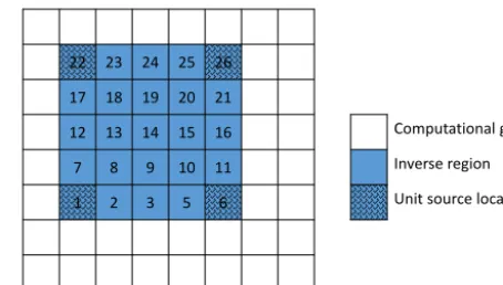
where w are the calculated water elevations using least squares, Eq. (5), andxdefine a unique identification for the computational grid of the forward model located inside the inverse regionX(Fig. 1). In this part, the combination of the algorithm with the least squares method is necessary to save the computational efforts.
22 23 24 25 26
17 18 19 20 21
12 13 14 15 16 Computational grid
7 8 9 10 11 Inverse region
1 2 3 5 6 Unit source locations
Figure 1. Example of a unique identification of the forward model
computational grid used for the second design parameters.
3.1 Genetic algorithm
GA is an optimization method that searches for an optimal value of a complex function by adopting the process of nat-ural evolution (Goldberg, 1989). It can be categorized as a type of stochastic optimization method and as a part of ar-tificial intelligence. In GA, the model parameters or deci-sion variables in the optimization are first transformed into a chromosome-like data structure that later evolves to form a better individual. The most common representation of design parameters in GA is their encoding into a binary string. There are three basic genetic operators in GA: selection, crossover, and mutation.
As described in Wetter and Wright (2003), in GA, finite lower and upper bounds ofX are discretized in the mesh
M(l,1), and all operators are such that the real value of any
point is an element ofM(l,1)∩X. Given a non-empty set X⊂Rnand a non-zeroM∈N,eXM is defined as the set of
all sequenceXwithMelements, e
XM=˙
n
{xi}Mi=1|xi∈X, i∈ {1, . . ., M}
o
. (10)
ConsiderB as the set containing all elements ofM(l,1)∩ X. Similarly,eBM is the set of all sequences in B withM
elements, e
BM=˙
n
yi M i=1
yi∈B, i∈ {1, . . ., M} o
. (11)
We denote k∈N as the generation number, M∈N as the population size,exk∈XeM as theMpoints in thekth
gener-ation,eyk∈eBM as the binary representation ofexk, andeyk,i denotes theith element ofeyk fori∈ {1, . . ., M}, which is a binary representation of a point inRn. The step-by-step
op-eration of the GA is described in the following:
Step (1): randomize the initial populationey0∈eBM ofM
randomly generated points. Then, evaluate alleyk according to the specified cost function; thus, a fitness function2:N× e
BM→RM computes a fitness value ofeyk.
Step (2): select a pair of individuals with the selection functionϑ:N×eBM→eB2. Individuals with better fitness
140°E 142°E 144°E 35°N
37°N 39°N 41°N
−7000 −6000 −5000 −4000 −3000 −2000 −1000 0
−8370 m 0 m
100 km
1 2 3
4 5 6 7
8
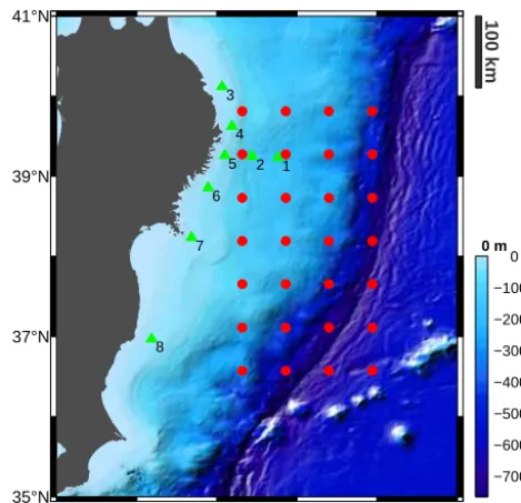
Figure 2. Study area and bathymetry profile. Red dots indicate unit
sources located throughout the inverse region. Green triangles with numbers are artificial observation stations.
Step (3): swap the bits (genes) between the selected in-dividuals (chromosomes) to produce new offspring,φ:N× e
B2×[0,1]→Be2with the crossover probabilitypr∈[0,1].
Step (4): the final genetic operator is termed mutation and aims to maintain genetic diversity. The mutation functionψ:
N×B×[0,1]→Balters a bit on individuals from its initial
state.
3.2 Pattern Search
Similar to GA, PS is an optimization method that does not require the gradient (derivative-free) of the problem to be optimized. The method was first introduced by Hooke and Jeeves (1961). Later, Torczon (1997) conducted studies to prove the convergence of PS using the theory of positive bases. The algorithm of PS used in this study is similar to that of Wetter and Write (2003), while the design parameters are identical to the GA optimization.
For the same optimization problem as formulated in Eqs. (8) and (9), the algorithm searches a lower cost func-tion value than f (xk), wherexk∈Xdenotes a solution at the current iterate and k∈N denotes the iteration number. The search takes place on the points in the set
γk=˙nx∈X
x=xk±1ks
ie
i, i∈ {1, . . ., n}
o
, (12)
where1k>0 is the mesh size factor,s∈Rn is a fixed
pa-rameter to scale the design papa-rameters, andeis the unknown approximation error. The rule to select a finite number of points inXon a mesh can be defined by the following:
M(x0, 1k)=˙
n
x+m1ksiei|i∈ {1, . . ., n}, m∈Z
o
, (13)
Figure 3. Gaussian basis function.
wherex0∈Xis the initial iterate.
The overall procedures of PS optimization can be elabo-rated as follows:
Step (1): initializex0∈Xand10>0, for which in our
case,x0is obtained from the GA’s output.
Step (2): iff x0
< f (xk)for somex0∈M(x0, 1k), then
setxk+1=x0and1k+1=1k.
Step (3): iff x0
≥f (xk)for allx0∈γk, the search
con-tinues withxk+1=xkand reduced mesh factor1k+1=12k.
The search should continue until a stopping condition is sat-isfied; e.g., the mesh has been refined a user-specified num-ber of time or less than a given tolerance.
4 Numerical experiments
We have conducted numerical experiments using an artificial tsunami source propagated on an actual bathymetry profile. An area extending from 140–145◦E and 35–41◦N is
cho-sen as the domain of interest. The selected domain resem-bles that used in most studies of tsunami waveform inver-sion for the 2011 Tohoku tsunami. The resolution of the nu-merical model is 1 arcmin, which is consistent with the res-olution of the bathymetry data obtained from the ETOPO1. ETOPO1 is a global relief model of the earth’s surface, which includes ocean bathymetry, available from the National Geo-physical Data Center of the National Oceanic and Atmo-spheric Administration (Amante and Eakins, 2009). There are eight artificial observation stations associated with the ac-tual location of gauges within the study area. The tsunami source is divided into 28 unit sources that are distributed uniformly around the actual epicenter of the 2011 Tohoku tsunami (Fig. 2).
4.1 Cost function
140°E 142°E 144°E 35°N
37°N 39°N
41°N 100 km
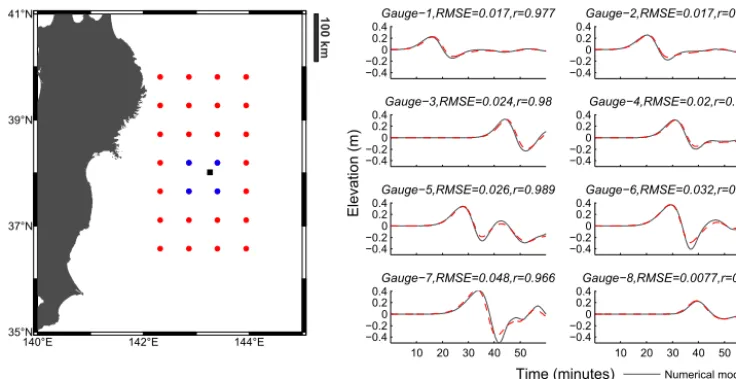
−0.4 −0.20 0.2 0.4Gauge−1,RMSE=0.017,r=0.977 −0.4 −0.20 0.2 0.4Gauge−2,RMSE=0.017,r=0.984 −0.4 −0.20 0.2 0.4Gauge−3,RMSE=0.024,r=0.98 −0.4 −0.20 0.2 0.4Gauge−4,RMSE=0.02,r=0.985 −0.4 −0.20 0.2 0.4Gauge−5,RMSE=0.026,r=0.989 Elevation (m) −0.4 −0.20 0.2 0.4Gauge−6,RMSE=0.032,r=0.983
10 20 30 40 50 −0.4
−0.20 0.2
0.4Gauge−7,RMSE=0.048,r=0.966
Time (minutes)
10 20 30 40 50 −0.4 −0.20 0.2 0.4Gauge−8,RMSE=0.0077,r=0.995 Numerical model Interpolation
Figure 4. Waveform interpolation. Left-hand figure shows selected location of a unit source indicated by a black square. Blue dots represent
the four nearest unit sources used in the interpolation. Right-hand figures are comparisons of waveforms between numerical model (solid black line) and interpolation (dashed red line) at the artificial gauges.
optimal solution. Here, we use a combination of root mean square error (RMSE) and Pearson correlation coefficient (r). While the RMSE is sensitive to amplitude matching, the cor-relation coefficient is more sensitive to phasing between the compared series (Barnston, 1992). The RMSE serves to ag-gregate the individual differences of data points into a single measure of predictive power, which is defined as follows:
RMSE= v u u t 1 n n X i=1
(di−yi)2, (14)
whereyis the predicted value by the model,dis the measure-ment data for eachith data point, or in our case, the wave-form generated by the artificial tsunami source, andnis the total number of data. The Pearson correlation coefficient is defined as a division of the covariance of the two variables by the product of their standard deviations:
r=
n
P
i=1
di−d·(yi−y)
s
n
P
i=1
di−d 2
·
n
P
i=1
(y−y)2
, (15)
whered andyrepresent the means ofdandy, respectively. The correlation or relevance of the data is measured using the valueR=0.5(r+1)to avoid negative values in the case of a decreasing linear relationship between the compared series. The fitness evaluation is subject to noise from various fac-tors that might lead the optimization towards unexpected so-lutions. The easiest technique to overcome such problems is by means of explicit averaging over a number of samples to smooth the cost function (Jin and Branke, 2005). As the best
Initial Green’s
function Genetic Algorithm Pattern Search
t t hV V g
xyt
Gi ,,
Random initial unit source positions
Interpolation
Converge? Yes No
T T G G G w 1
Update Gix,y,t
Finish GTG GT w 1
t t hV V g GA’s outputs Interpolation
Update Gix,y,t
T T G G G w 1
Optimized unit source positions
Final Green’s function
Figure 5. Flowchart of model development procedure.
solution or closest fit is indicated by RMSE→0 andR→1, the final cost function is a summation of the mean of thetth sample over the time windowT of Eqs. (14) and (15), which can be written as follows:
E= N X k=1 " 1 T T X t=1
RMSEt+(1−Rt)
#
k
, (16)
wherek denotes the respective time window and N is the total number of windows.
4.2 Basis function
A Gaussian shape with 1 m amplitude is used as the basis function for each unit source (Liu and Wang, 2008). Provid-ing ai as the amplitude of a unit source with the centroid
positions ofxi andyi, the basis function can be written as
follows:
zi(x, y)=aiexp
"
−(x−xi)
2+(y−y i)2
2σ2
#
(a) Target source
140°E 142°E 144°E
35°N 37°N 39°N 41°N
−1.5 −1 −0.5 0 0.5 1 1.5 2
−1.76 m 2.32 m
100 km
(b) Least squares
140°E 142°E 144°E
35°N 37°N 39°N 41°N
−1.5 −1 −0.5 0 0.5 1 1.5
−1.76 m 2.1 m
100 km
(c) GAPSu
140°E 142°E 144°E
35°N 37°N 39°N 41°N
−1.5 −1 −0.5 0 0.5 1 1.5
−1.76 m 2.12 m
100 km
(d) GAPSr
140°E 142°E 144°E
35°N 37°N 39°N 41°N
−1.5 −1 −0.5 0 0.5 1 1.5
−1.8 m 2.18 m
100 km
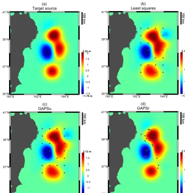
Figure 6. Sea surface deformation. Gray dots indicate the centroid of unit sources. (a) Artificial tsunami source as the target to be
approxi-mated, (b) inverted source using least squares method, (c) GAPSu model, (d) GAPSr model.
wherezi(x, y) is the initial water surface corresponding to
the ith unit source, x andy are the locations of computa-tional grids, andσ is the spread of the blob with a length of 40 km (Fig. 3). The specified length should satisfy the long wave assumption(h/L <0.05), i.e., the wavelength should be greater than 20 times the average water depth.
4.3 Model development
For the first design parameters, the optimization is performed merely to search the water elevation or initial amplitudes of each unit source. For this case, the Green’s function is constructed based on the initial 28 unit sources, separated by a uniform distance of 60 km, which is identical to that used in the least squares inversion. Hereafter, the first model will be termed the Genetic Algorithm Pattern Search for uniform source distribution (GAPSu). The purpose of this model is simply to compare the performance of the proposed
global optimization method with the traditional least squares method in the same model design and environment.
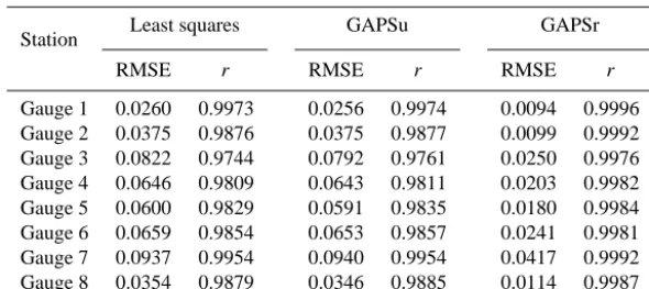
Table 1. Summary of statistical evaluations based of the proposed cost function.
Station Least squares GAPSu GAPSr
RMSE r RMSE r RMSE r
Gauge 1 0.0260 0.9973 0.0256 0.9974 0.0094 0.9996 Gauge 2 0.0375 0.9876 0.0375 0.9877 0.0099 0.9992 Gauge 3 0.0822 0.9744 0.0792 0.9761 0.0250 0.9976 Gauge 4 0.0646 0.9809 0.0643 0.9811 0.0203 0.9982 Gauge 5 0.0600 0.9829 0.0591 0.9835 0.0180 0.9984 Gauge 6 0.0659 0.9854 0.0653 0.9857 0.0241 0.9981 Gauge 7 0.0937 0.9954 0.0940 0.9954 0.0417 0.9992 Gauge 8 0.0354 0.9879 0.0346 0.9885 0.0114 0.9987
Asano, 2014). An example of the interpolation results, com-plete with statistical evaluations in terms of RMSE andr, is shown in Fig. 4. Despite the satisfying results, based on the measure of fitness shown by the interpolation method (over-all RMSE<0.048 m andr >0.966), the small errors might be amplified in the solution because of the ill-posed prob-lem. Consequently, further improvements should be made to suppress the generated errors.
An artificial tsunami source is used to test our method (Fig. 6a). Instead of using a simpler profile produced by the Okada’s solution, we generate a more complex shape from a superposition of 10 unit sources with random amplitudes and positions located inside the inverse region. We purposely limit the number of unit source to avoid generating shorter wavelengths than the prescribed long wave assumption. For the regular Green’s function (first design parameter), using only 10 unit sources is insufficient to reconstruct the tar-get profile. Consequently, the number of unit source should be increased. The decision of using 28 unit sources in both design parameters is for the purpose of model performance comparisons that will be further discussed in the Results and discussion section. The approximation of this initial profile is performed using unconstrained, traditional least squares in-version, GAPSu, and GAPSr. However, GAPSr is the most important part in this study; therefore, we focus our discus-sion on the GAPSr model. The development of the GAPSr model depicted in the flowchart (Fig. 5) can be summarized as follows:
1. Construct the initial Green’s function.
2. Initialize the GAPSr model by randomly distributing the unit source locations. The search of the optimal location is bounded by the area of the inverse region.
3. Perform interpolation and update the Green’s function. 4. Evaluate the fitness by performing the least squares
in-version.
5. After reaching the stopping criteria, the forward numer-ical modeling is run again for each of the optimized unit
sources to avoid errors generated from the interpolation result. Subsequently, the inversion is performed for the final time.
5 Results and discussion
Overall, all models can produce a relatively good estimation of the targeted sea surface deformation. This is likely because they are applied to an ideal case with artificial conditions and settings, except for bathymetry. For instance, the target source was generated from the same Gaussian shape as that used to construct the Green’s function. Therefore, the task is more straightforward as fewer complexities are encountered. In the real case, however, alternative distributions to repre-sent the initial water height should be considered because the tsunami source does not always follow the Gaussian distribu-tion. This may have a profound effect on the result of the first design parameter, but less significant for the second design parameter as a superposition of unit sources with random lo-cations allows to approximate any surface profile regardless of their shape. Nevertheless, in this study, the use of the ideal case has allowed us to assess the advantage of the proposed method in a more detailed manner.
suc-Gauge8
Time (minutes)
10 20 30 40 50 60 70 80 90
−0.5 0 0.5
Gauge7
−1 0 1 2 3
Gauge6
−0.5 0 0.5 1
Gauge5
Elevation (m)−0.5 0 0.5
Gauge4
−0.5 0 0.5
Gauge3
−0.5 0 0.5 1
Gauge2
−0.4 −0.20 0.2 0.4
Gauge1
−0.5 0 0.5
1 Target Least squares GAPSu GAPSr
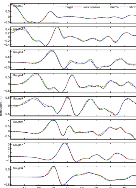
Figure 7. Comparison of waveforms at gauges. Gray bar above the
time axis indicates the time range for the inversion.
cessfully promoted for the case of tsunami waveform inver-sion. This was because the optimization method was applied to a nonlinear inverse problem of actual measurement data. Accordingly, the appraisal of such a method can be clearly defined.
Spurious uplifts and subsidence of the water surface pro-file are generated in both the least squares and GAPSu model results (see Fig. 6b and c). One may argue that the spec-ified spatial resolution of the unit sources is too coarse to represent the complete form of the target source. A denser distribution of unit sources should improve the results; how-ever, it might also introduce other problems. A large num-ber of model parameters (unknown parameters), which are proportional to the degrees of freedom in the optimization, are liable to cause the solution to become easily entrapped in a local optimum. Without a smoothing constraint, the re-sult of the tsunami waveform inversion might be bumpy and non-physical, especially for cases with high spatial resolution (Wu and Ho, 2011). In other studies on tsunami waveform inversion by Baba et al. (2005) and Wu and Ho (2011), an equality constraint was imposed to maintain the smoothness of the inverted parameters to satisfy the long wave assump-tion, while by Saito et al. (2010) and Gusman et al. (2010)
−2 0 2 4
−2 0 2 4
Target
Least squares
Y=0.9831X+0.0068 r =0.9908 RMSE =0.0622
Fit 95% PI Y=X
−2 0 2 4
−2 0 2 4
Target
GAPSu
Y=0.9830X+0.0069 r =0.9910 RMSE =0.0615
Fit 95% PI Y=X
−2 0 2 4
−2 0 2 4
Target
GAPSr
Y=0.9889X+0.0018 r =0.9988 RMSE =0.0224
Fit 95% PI Y=X
Figure 8. Scatter plots of each inversion method with respect to the
waveforms of the target source at all gauges.
the constraint was used to obtain stable solutions. However, such constraint might restrict the exploration throughout the feasible search space and render the discovery of an opti-mum solution more difficult. Another plausible explanation for the unsatisfactory results of the least squares and GAPSu model is simply that the equidistant unit sources in the regu-lar Green’s function confines the search for optimality. This can be proven by the result of the GAPSr model, for which the same number of model parameter (28 unit sources) with random locations yields a much better estimation.
op-timization response time. The solution and convergence are strongly dependent on the random initial state.
6 Conclusions
Estimations of tsunami sea surface deformation using a global optimization method with a stochastic nature have been conducted. Our numerical experiments using the GAPSu model revealed that the use of such methods for a linear system with standard design parameters, as in or-dinary tsunami waveform inversions, is redundant and pro-motes trivial improvements. In contrast, the different design parameters in our proposed method (GAPSr), which was ap-plied to determine the optimum location of the unit sources prior to the inversion, demonstrated considerable improve-ments in the accuracy. The random location of unit sources permitted the inversion to produce a more precise approxima-tion of the initial sea surface deformaapproxima-tion without violating the general assumption of long wave theory.
The involvement of stochastic processes in the opti-mization increased the ability to reveal uncertainties in the tsunami source, which are difficult to discern using deterministic approaches. However, as the signature of typical stochastic optimizations, the optimization response time is erratic because of the strong dependency on the initial state. Using a current standard desktop computer, the required computing time varied from 5 to 10 min. Thus, a more sophisticated computer would be needed to ensure the effectiveness of the method when applied in a real-time application. Nevertheless, the results have demonstrated the efficacy of the method for post-event studies of tsunamis, because it can provide better estimations of the coseismic sea surface deformation compared with traditional tsunami waveform inversion methods.
Edited by: I. Didenkulova
Reviewed by: A. Gusman and two anonymous referees
References
Aida, I.: Numerical estimation of a tsunami source, Zisin 2 (J. Seism. Soc. Japn.), 25, 343–352, 1972.
Amante, C. and Eakins, W.: ETOPO1 1 arc minute global relief model: procedures, data sources and analysis, NOAA technical memorandum NESDIM NGDC-24, 19 pp., 2009.
Baba, T., Cummins, P. R., and Hori, T.: Compound fault rupture during the 2004 off the Kii Peninsula earthquake (M 7.4) inferred from highly resolved coseismic sea-surface deformation, Earth Planet. Space, 57, this issue, 167–172, 2005.
Barnston, A. G.: Correspondence among the Correlation, RMSE, and Heidke Forecast Verification Measures; Refinement of the Heidke Score, Weather Forecast., 7, 699–709, 1992.
Costa, L., Santo, I., Denysiuk, R., and Fernandes, E. M. G. P.: Hybridization of a Genetic Algorithm with a Pattern Search Augmented Lagrangian Method, in: International Conference on
Engineering Optimization, Lisbon, Portugal, 6– 9 September , 2010.
Geist, E. L.: Complex earthquake rupture and local tsunamis, J. Geophys. Res., 107, ESE2-1–ESE2-16, doi:10.1029/2000JB000139, 2002.
Geist, E. L.: Local Tsunami Hazards in the Pacific Northwest from Cascadia Subduction Zone Earthquakes, US Geological Survey Professional Paper, 1661-B, 17 pp., 2005.
Goldberg, D. E.: Genetic algorithms in search, optimization and ma-chine learning, Longman Publishing Co., New York, 1989. Gusman, A. R., Tanioka Y., Kobayahi, T., Latief, H., and Pandoe,
W.: Slip distribution of the 2007 Bengkulu earthquake inferred from tsunami waveforms and InSAR data, J. Geophys. Res., 115, B12316, doi:10.1029/2010JB007565, 2010.
Gusman, A. R., Fukuoka, M., Tanioka Y., and Sakai, S. I.: Effect of the largest foreshock (Mw 7.3) on triggering the 2011 To-hoku earthquake (Mw 9.0), Geophys. Res. Lett., 40, 497–500, doi:10.1002/grl.50153, 2013.
Hooke, R. and Jeeves, T. A.: Direct search solution of numerical and statistical problems, J. Assoc. Comp. Mach, 8, 212–229, 1961. Jin, Y. and Branke, J.: Evolutionary optimization in uncertain
en-vironments – a survey, IEEE Trans. Evol. Comput., 9, 303–317, 2005.
Koike, N., Kawata, Y., and Imamura, F.: Far-field tsunami poten-tial and a real-time forecast system for the Pacific using the in-version method, Natural Hazards, Kluwer Academic Publishers, 423–436, 2003.
Liu, P. L. F. and Wang, X.: Tsunami source region parameter identi-fication and tsunami forecasting, J, Earthquake Tsunami, 2, 87– 106, 2008.
Mansinha, L. and Smylie, D. E.: The displacement fields of inclined faults, Bull. Seismol. Soc. Am., 61, 1433–1440, 1971.
Mulia, I. E. and Asano, T.: Determination of the initial sea sur-face deformation caused by a tsunami using Genetic Algorithm, Coastal Engineering Proceedings, The 34th International Confer-ence on Coastal Engineering, Seoul, Korea, 15–20 June 2014, 1, currents.10, doi:10.9753/icce.v34.currents.10, 2014.
Okada, Y.: Surface deformation due to shear and tensile faults in a half-space, Bull. Seismol. Soc. Am., 75, 1135–1154, 1985. Payne, J. L. and Eppstein, M. J.: A hybrid genetic algorithm with
pattern search for finding heavy atoms in protein crystals, in: Pro-ceedings of conference on genetic and evolutionary computation, Washington, DC, USA, 377–384, 2005.
Piatanesi, A. and Lorito, S.: Rupture process of the 2004 Sumatra– Andaman Earthquake from tsunami waveform inversion, Bull. Seismol. Soc. Am., 97, S223–S231, doi:10.1785/0120050627, 2007.
Romano, F., Piatanesi, A., Lorito S., and Hirata, K.: Slip distribution of the 2003 Tokachi-oki Mw 8.1 earthquake from joint inversion of tsunami waveforms and geodetic data, J. Geophys. Res. 115, B11313, doi:10.1029/2009JB006665, 2010.
Saito, T., Satake, K., and Furumura, T.: Tsunami waveform inversion including dispersive waves: the 2004 earthquake off Kii Peninsula, Japan, J. Geophys. Res., 115, B06303, doi:10.1029/2009JB006884, 2010.
Satake, K., Baba, T., Hirata, K., Iwasaki, S., Kato, T., Koshimura, S., Takenaka, J., and Terada, Y.: Tsunami source of the 2004 off the Kii Peninsula earthquakes inferred from offshore tsunami and coastal tide gauges, Earth Planet. Space, 57, this issue, 173–178, 2005.
Torczon, V. J.: On the convergence of pattern search algorithms, SIAM J. Optimiz., 7, 1–25, 1997.
Tsushima, H., Hirata, K., Hayashi, Y., Tanioka, Y., Kimura, K., Sakai, S., Shinohara, M., Kanazawa, T., Hino, R., and Maeda, K.: Near-field tsunami forecasting using offshore tsunami data from the 2011 off the Pacific coast of Tohoku Earthquake Hi-roaki Tsushima, Earth Planet. Space, 63, 821–826, 2011. Voronina, T.: Reconstruction of initial tsunami waveforms by a
truncated SVD method, J. Inv. Ill-Posed Problems, 19, 615–629, 2011.
Wetter, M. and Wright, J.: Comparison of a generalized pattern search and a genetic algorithm optimization method, in: Proceed-ings of the Eighth IBPSA Conference, edited by: Augenbroe, G. and Hensen, J., Vol. III. NL: Eindhoven, 1401–1408, 2003. Wu, T.-R. and Ho, T.-C.: High resolution tsunami inversion for 2010
Chile earthquake, Nat. Hazards Earth Syst. Sci., 11, 3251–3261, doi:10.5194/nhess-11-3251-2011, 2011.