Protein Hydrogen Exchange, Dynamics, and Function

(1)

University of Pennsylvania

ScholarlyCommons

Publicly Accessible Penn Dissertations

1-1-2012

Protein Hydrogen Exchange, Dynamics, and

Function

John Skinner

University of Pennsylvania, [email protected]

Follow this and additional works at:http://repository.upenn.edu/edissertations

Part of theBiochemistry Commons, and theBiophysics Commons

This paper is posted at ScholarlyCommons.http://repository.upenn.edu/edissertations/582 For more information, please [email protected].

Recommended Citation

(2)

Protein Hydrogen Exchange, Dynamics, and Function

Abstract

Models derived from X-ray crystallography can give the impression that proteins

are rigid structures with little mobility. NMR ensembles may suggest a more dynamic

picture, but even these represent a rather narrow range of possibilities close to the lowest

energy state. In reality proteins participate in a wide range of dynamics from the subtle

and rapid sidechain dynamics that occur in nanoseconds in the PDZ signaling domain to

the large and slow rearrangement of secondary structure that takes days in the mitotic

checkpoint protein Mad2. Between these extremes are motions on time scales typically

associated with protein function, such as those in SNase monitored by hydrogen

exchange. The dynamic character of several protein systems, including PDZ domain,

Calmodulin, SNase, and Mad2, were explored using a variety of biophysical techniques.

This broad investigation demonstrates the dynamic variability between and within

proteins. The study of PDZ and Calmodulin illustrates how a computational technique

can recapitulate experimental results and provide additional insight into signal

transduction. The case of SNase shows that HX NMR data can be exploited to reveal

protein dynamics with unprecedented detail. The Mad2 system highlighted some of the

pitfalls associated with this technique and some alternative strategies for investigating

protein dynamics.

Degree Type Dissertation

Degree Name

Doctor of Philosophy (PhD)

Graduate Group

Biochemistry & Molecular Biophysics

First Advisor S Walter Englander

(3)

Second Advisor Ben E. Black

Keywords

CLEANEX-PM, HX, Hydrogen exchange, Mad2, Protein folding, Pump probe molecular dynamics

Subject Categories Biochemistry | Biophysics

(4)

PROTEIN HYDROGEN EXCHANGE, DYNAMICS, AND

FUNCTION

John J. Skinner

A DISSERTATION in

Biochemistry and Molecular Biophysics

Presented to the Faculties of the University of Pennsylvania in

Partial Fulfillment of the Requirements for the Degree of Doctor of Philosophy

2012

Supervisor of Dissertation Co-Supervisor of Dissertation

______________________ _______________________

S. Walter Englander Ben E. Black,

Professor Assistant Professor

Biochemistry and Biophysics Biochemistry and Biophysics

Graduate Group Chairperson ______________________ Kate Ferguson

Associate Professor Physiology

Dissertation Committee Members Kim Sharp, Associate Professor,

Biochemistry and Biophysics

A. Joshua Wand, Benjamin Rush Professor, Biochemistry and Biophysics

Ravi Radhakrisnan, Associate Professor, Bioengineering

P. Leslie Dutton, Eldrige Reeves Johnson Professor, Biochemistry and

Biophysics

Greg Van Duyne, Jacob Gershon-Cohen Professor, Biochemistry and Biophysics

(5)

ii

(6)

iii

ACKNOWLEDGMENTS

I would like everyone who contributed this work. Foremost, I would like to thank

my advisers Walter Englander and Ben Black who provided guidance throughout most of

my graduate career and Kim Sharp who provided guidance during the early phase of my

graduate studies. I would also like to thank Stacey Wood, Leland Mayne, Ninad Prabhu,

and Yibing Wu for the training and assistance they provided. In addition to sharing her

HXMS data with me, Sandya Ajith proved to be a valuable friend at all times. Samuel

Getchell in my tribulations of protein purification and partnered with Brian Wexler to

collect some of the Mad2 kinetic data that has been included in this thesis. I would also

like to thank J. Nathan Scott for his patience in answering my endless Matlab questions.

Many thanks to those who provided materials, data, and assistance including Sergei

Vignodagrav who provided Rhodamine B flourophore, Lee Solomon who helped me

incorporate the fluorophore into a synthetic peptide, and Bogumil Zelent who guided me

in my fluorescence measurements. Thanks to Michele Vendruscolo and Liu Tong for

providing some of the HX predictions used in Chapter 4 and to Tobin Sosnick who not

only allowed me to use the NMR facility at University of Chicago, but also allowed me

to stay in his home while doing so. I would also like to thank all the members of the

Englander and Black labs for helpful discussions throughout my time in those labs.

Finally, I want to thank my dog Montana who made lab all the more enjoyable with his

(7)

iv

ABSTRACT

PROTEIN HYDROGEN EXCHANGE, DYNAMICS, AND

FUNCTION

John J. Skinner S. Walter Englander

Ben E. Black

and rapid sidechain dynamics that occur in nanoseconds in the PDZ signaling domain to

the large and slow rearrangement of secondary structure that takes days in the mitotic

checkpoint protein Mad2. Between these extremes are motions on time scales typically

associated with protein function, such as those in SNase monitored by hydrogen

exchange. The dynamic character of several protein systems, including PDZ domain,

Calmodulin, SNase, and Mad2, were explored using a variety of biophysical techniques.

(8)

v

LIST OF TABLES

Table 2.1 Phase Delay of a 10 ps Pump Applied to H76 of PDZ………..43

Table 2.2 Summary of changes in coupling due to mutations in PDZ domain protein….46 Table 3.1 pH-independent log k0 rates for SNase………..77

Table 5.1 SNase protection factors………..133

Table 6.1 Mad2 mutants used in this study………..157

Table 6.2 Temperature dependent interconversion rates………...173

Table 6.3 Rates of decay for O-Mad2 and rise of C-Mad2 peaks………...175

(14)

xi

LIST OF FIGURES

Figure 2.1 Fluctuation power spectra of some atomic motions in CaM………30

Figure 2.2 Coupling profiles for CaM with the C helix pumped………...31

Figure 2.3 Coded structural representation of CaM………...32

Figure 2.4 Coded structural representation of PDZ domain protein………..32

Figure 2.5 PDZ domain coupling profiles……….34

Figure 2.6 Plot of coupling strength vs. Cα–Cα distance for PDZ domain pumped at H76……….35

Figure 2.7 Percentile analysis of similarity of coupling profiles for CaM………37

Figure 2.8 Percentile analysis of similarity of coupling profiles for PDZ………38

Figure 2.9 Fluctuation cross-correlation for PDZ domain protein from a control simulation………...41

Figure 2.10 Time cross-correlation functions for Cα atoms in PDZ domain………42

Figure 2.11 Time autocorrelation functions for atomic motions in CaM with implicit or explicit solvent………...45

Figure 3.1CLEANEX-PM pulse sequence………...69

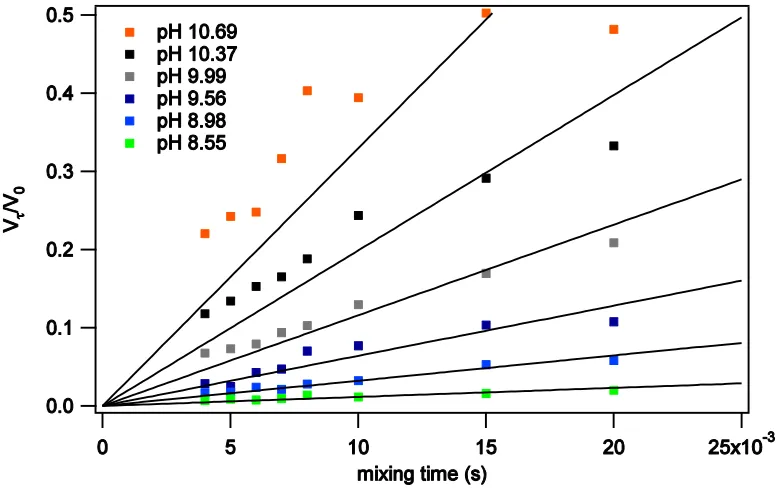
Figure 3.2 Uncorrected peak volumes as a function of mixing time for SNase Gly86….73 Figure 3.3 Peaks volumes after background signal has been subtracted………...73

Figure 3.4 Linear fits to time courses………74

Figure 3.5 Best fit lines using Eq. 3.1 with the approximation R1A = 0………75

Figure 3.6 Best fit lines using Eq. 3.1 to fit both kex and R1A………75

Figure 3.7 Fit for all pH’s simultaneously……….76

Figure 3.8 Final pH dependent fitting step………77

Figure 3.9 kex determined from linear slope vs final kex………78

(15)

xii

Figure 4.1 Log kex vs pH for SNase………...87

Figure 4.2 Protection factors as a function of distance to the protein surface…………...91

Figure 4.3 ΔG of deprotonation calculated by Qnifft compared to previously published ΔpKa calculations for rubredoxin………..93

Figure 4.4 ΔG of deprotonation calculated by Qnifft compared to previously published ΔpKa calculations for CI2 and FKBP12………93

Figure 4.5 ΔG of deprotonation calculated by Qnifft compared to previously published ΔpKa calculations for ubiquitin……….94

Figure 4.6 ΔpKa from electrostatic calculations vs measured HX rates for SNase……...95

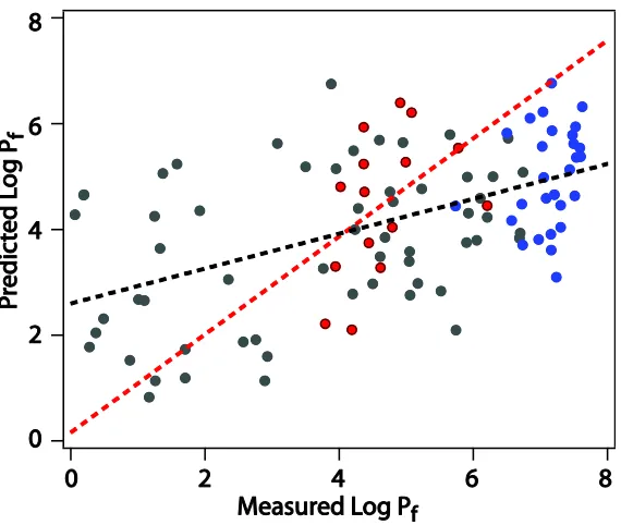
Figure 4.7 Measured log Pf vs log Pf predicted from local packing density……….99

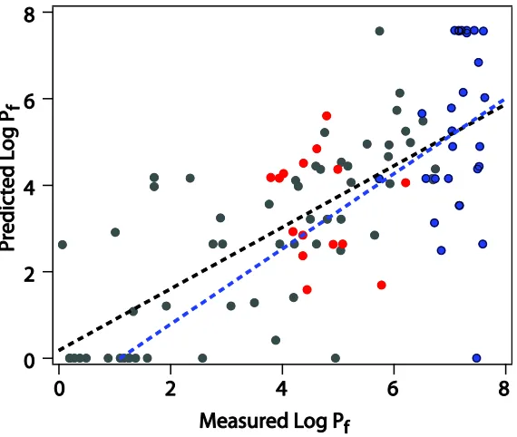
Figure 4.8 Log Pf predicted by H-COREX vs measured log Pf………..102

Figure 5.1 Hydrogen bond inventory for SNase………..113

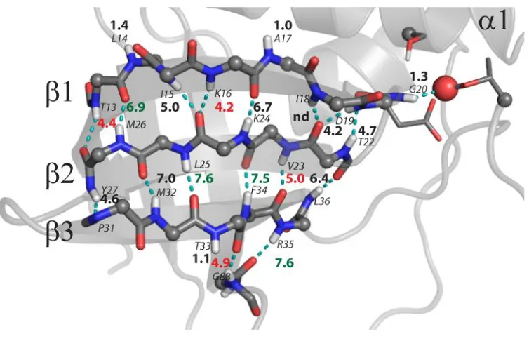
Figure 5.2 HX protection pattern indicating global unfolding on one face of the SNase β -barrel………115

Figure 5.3 Heterogeneous exchange in the SNase β-barrel……….118

Figure 5.4 Sidechains between solvent and Val23 and Leu25………120

Figure 5.5 HX behavior in the SNase α-helices………...121

Figure 5.6 Cooperative motion in the α1/β4 loop………124

Figure 5.7 An internal water molecule and several loops………125

Figure 5.8 Loops with internal waters……….127

Figure 5.9 Electron density map surrounding Thr82………..….128

Figure 5.10 The Asn138 protection factor is consistent with the SNase NMR structure………129

Figure 5.11 Exchange mechanisms displayed on the structure of SNase………131

Figure 6.1 The mitotic checkpoint ensures equal partitioning of chromosomes in anaphase………...146

(16)

xiii

Figure 6.3 Mad2 unfolding and refolding considerations………155

Figure 6.4 Mad2 purification gel……….161

Figure 6.5 Anion exchange and size exclusion chromatograms for Mad2RQ_{…………..}₁₆₈

Figure 6.6 CD spectra forMad2RF………...169

Figure 6.7 Mad2 interconversion……….170

Figure 6.8 Structure highlighting interactions involving the residues that have been mutated in Mad2RQ_{and Mad2}RF_………_..172

Figure 6.9 1_H-15_{N HSQC spectra for Mad2}_{……….174}

Figure 6.10 1H-15N peaks that shift from open to closed conformations mapped onto O-Mad2 and C-O-Mad2 structures………...177

Figure 6.11 Electrostatic analysis of differences in binding affinity for O-Mad2 and C-Mad2………179

Figure 6.12 HX mass spectroscopy results for Mad2RF_………._..184

Figure 6.13 2D projections of HNCA and HN(CO)CA spectra………..…186

Figure 6.14 FCS results for RhB-MBP1 binding to Mad2………..188

(17)

xiv

ABBREVIATIONS

APC – Anaphase promoting complex/cyclosome BSA – Bovine serum albumin

CaM - Calmodulin CD – Circular dichroism

Cdc20 – Cell division cycle 20. A protein regulated by Mad2 C-Mad2 – Closed conformation of Mad2

FCS – Fluorescence correlation spectroscopy FPLC – Fast pressure liquid chromatography

GdmCl – Guanidinium chloride

HSQC – Heteronuclear single quantum coherence HX – Hydrogen exchange

IPTG –Isopropyl β-D-1-thiogalactopyranoside LB – Lysogeny broth

Mad1 – Mitotic arrest deficient protein 1 Mad2 – Mitotic arrest deficient protein 2

Mad2ΔC_–_{Mad2 with the last 10 residues truncated}

Mad2ΔN_–_{Mad2 with the first 10 residues truncated} Mad2RF– Mad2 R133A/F141A mutant

Mad2RQ_–_{Mad2 R133E/Q134A mutant}

MBP1 – Mad2 binding peptide 1 MCC – Mitotic checkpoint complex MD – Molecular dynamics

(18)

xv

NMR – Nuclear Magnetic Resonance O-Mac2 – Open conformation of Mad2

PDZ – PSD-95, Discs Large, Zo-1. A common protein domain. Pf– Protection factor

PMSF - Phenylmethanesulfonylfluoride PPMD – Pump-probe molecular dynamics

RhB-MBP1 – MBP1 covalently linked to a Rhodamine B derivative SEC – Size exclusion chromatography

SNase – Staphylococcal nuclease

WT Mad2 –Post PreScission™ cleavage form of Mad2. Pro has been inserted at the +2

(19)

1 CHAPTER 1

INTRODUCTION

1. Protein Dynamics

and rapid sidechain dynamics that occur in nanoseconds in the PDZ signaling domain (1)

to the large and slow rearrangement of secondary structure that takes days in the mitotic

checkpoint protein Mad2 (2). Between these extremes are motions on time scales

typically associated with protein function, such as those in SNase monitored by hydrogen

exchange.

1.1 Allostery

Allosteric effects require interactions between spatially separated sites without

obvious structural reconfiguration. The mechanism underlying this process is not

completely understood. Allostery can be thought of as occurring by modulation of

dynamic pathways (3) or by perturbing the overall protein ensemble (4). These models

(20)

2

distal domains to somehow communicate with one another and a pathway view is

compatible with multiple routes.

One popular method for investigating protein dynamics is to apply molecular

dynamics (MD) simulations. Unfortunately, it is difficult to parse the dynamics relating

to allosteric regulation from the other dynamics occurring throughout a protein. Chapter 2

describes a novel technique called pumped-probe MD (ppmd; (1) that allows for the

detection of allosteric pathways by applying a low frequency pumping force to an MD

simulation and monitoring how the force transfers through the protein.

1.2 Relating Protein Dynamics to Hydrogen Exchange Data

Hydrogen exchange (HX) has proved to be a valuable technique for studying

protein dynamics. What makes this method so powerful is that it is only sensitive to the

populations in which a backbone amide is exposed to solvent. For most residues this

corresponds to higher energy states that become populated anywhere from 10-1_{to 10}-9_of

the time. Because HX rates are known for unfolded peptides (5, 6), HX rates measured

for folded proteins can be translated into stability constants. Combining this technique

with 2D NMR (7) allows for the determination of residue resolved stabilities.

HX rates have often been associated with protein folding (8). However, faster

rates often result from local motions that occur on timescales relevant to many protein

functions. Obtaining HX rates for marginally protected and unprotected residues has

(21)

3

made to fitting algorithms. Chapter 3 describes a novel algorithm for accurately

determining HX rates from magnetization transfer experiments.

Several groups have applied models to relate HX data to protein structure (12–

14). Chapter 4 evaluates the effectiveness of these models at predicting HX rates for

Staphylococcal nuclease (SNase). The failure of each of these methods to accurately

predict HX rates inspired the detailed examination of the SNase structure in relation to

measured HX rates, discussed in Chapter 5. The structural analysis leads to several

general conclusions including that residues with multiple layers of secondary structure

between themselves and the edges of those structures tend to exchange as cooperative

units regardless of the proximity to solvent and that an amide can hydrogen bond to a

water molecule without becoming HX competent. In several cases involving local

structural fluctuations detailed motions could be inferred from the context of nearby

residues based on HX rates and local structure.

1.3 Conformational Switching

Mad2 is one of a handful of proteins, known as metamorphic proteins (15), that

undergo a drastic structural rearrangement as part of their function. Other such proteins

include RNA polymerase (16, 17), viral glycoprotein (18), chloride ion channel (19),

lysozyme (20), and chemokine lymphotactin (21, 22). Of this group, Mad2 is the only

protein known to exist in both of its conformations in the absence of ligand or

environmental perturbation. In the case of Mad2 this conformation change includes the

(22)

4

Conformational switching is required for Mad2 to bind either its upstream effector or the

protein Mad2 regulates (23). While this switching is necessary for Mad2’s function as a

mitotic regulatory protein, the structural details of this transition have not been described

(24). Chapter 6 of this thesis describes an investigation of the intermediate I-Mad2

conformation by various biophysical techniques.

2. Hydrogen Exchange Theory

2.1 Hydrogen Exchange Rates

Backbone amides have a pKa >18, which means they are in constant exchange

with solvent even though the population is never significantly deprotonated. Above pH

~3 HX is catalyzed by OH-_{, thus the rate of HX increases by 10-fold for each pH unit. N}

-is a stronger base than OH- by >100-fold so amide NH to OH- ion collision occurs >100

times before the proton is actually carried away. For a polypeptide chain in a random

coil HX rates at pH 7 at 0 o_{C are about 1 s}-1_{. These rates are dependent on sequence,}

temperature, pH and isotope, which have been accurately calibrated (5, 6).

When an amide is hydrogen bonded it is isolated from solvent and therefore

completely protected from attack by OH- catalyst. HX occurs only when the amide

samples a state in which it is exposed to solvent. The resulting HX rate can be described

as follows:

(23)

5

where kch is the known HX rate for the amide if it were in a random coil, kop is the rate

for opening the amide to solvent, and kcl is the reclosing rate. In most cases kcl >> kch and

kcl>>kop, which reduces Eq. 1 to

kobs = kopkch/kcl Eq. 1.2

This is known as the EX2 case. Since kch is known, one can determine the ratio kop/ kcl

which is trivially converted into stability against the opening reaction. It should be noted

that this analysis assumes that the exposed state exchanges at the same rate as a random

coil, which may not be true in all cases (discussed in Chapter 5).

When pH is high and kcl is slow (kcl<< kch), we enter the EX1 regime. Here Eq.

1.1 reduces to

kobs = kopkch/ kch = kop Eq. 1.3

EX1 behavior has only been observed in the most stable regions of very stable proteins.

2.2 Mechanisms of Amide Exposure

The stability and (un)folding rates of proteins are typically determined by

methods that analyze the protein as a whole or possibly one specific region of the protein.

NMR HX allows the determination of these properties on a residue-by-residue basis. This

has led to the observation that hydrogen bonded amides exchange by three different

(24)

6

For amides that exchange by global unfolding, HX exhibits the same stability, denaturant

dependence, and unfolding rate (kop) as the protein as a whole as measured by other

methods (25, 26). Collectively, these residues appear to represent the first fragment or

“foldon” of the protein to fold and the last to unfold (8). This first foldon may be stable independently of the rest of the protein and can provide the nucleus or template upon

which the rest of the structure can form (27).

Amides that exchange by a sub-global unfolding mechanism have a lower

stability and shallower denaturant dependence than their global counterparts (27). The

shallower denaturant dependence is due to the partially unfolded conformers exposing

less surface area than the globally unfolded state. When these amides are clustered into

foldons by their equilibrium and kinetic properties and mapped onto the protein, they are

typically found to be clustered spatially as well. These units are thought to build upon the

global scaffold and one another in a sequential manner (28).

Exchange by local fluctuations is the least understood of the three mechanisms.

These residues exhibit no denaturant dependence, which presumably means little or no

additional surface area is exposed in the exchange competent state. From the perspective

of one studying protein folding, local fluctuations are an annoyance which one tries to

circumvent by adding denaturant until the stability becomes such that the amide

exchanges by way of a more interesting global or sub-global unfolding. However, these

fluctuations may play an important role in other protein functions.

(25)

7

The dynamic character of several protein systems, including PDZ domain,

Calmodulin, SNase and Mad2, were explored using a variety of biophysical techniques.

protein dynamics.

4. Bibliography

1. Sharp, K., and J.J. Skinner. 2006. Pump-probe molecular dynamics as a tool for

studying protein motion and long range coupling. Proteins. 65: 347-361.

2. Luo, X., Z. Tang, G. Xia, K. Wassmann, T. Matsumoto, J. Rizo, and H. Yu. 2004.

The Mad2 spindle checkpoint protein has two distinct natively folded states. Nat

Struct Mol Biol. 11: 338-345.

3. del Sol, A., C.-J. Tsai, B. Ma, and R. Nussinov. 2009. The Origin of Allosteric

Functional Modulation: Multiple Pre-existing Pathways. Structure. 17: 1042-1050.

4. Wrabl, J.O., J. Gu, T. Liu, T.P. Schrank, S.T. Whitten, and V.J. Hilser. 2011. The

role of protein conformational fluctuations in allostery, function, and evolution.

(26)

8

5. Bai, Y., J.S. Milne, L. Mayne, and S.W. Englander. 1993. Primary structure effects

on peptide group hydrogen exchange. Proteins. 17: 75-86.

6. Connelly, G.P., Y. Bai, M.F. Jeng, and S.W. Englander. 1993. Isotope effects in

peptide group hydrogen exchange. Proteins. 17: 87-92.

7. Wagner, G., and K. Wüthrich. 1982. Amide proton exchange and surface

conformation of the basic pancreatic trypsin inhibitor in solution: Studies with

two-dimensional nuclear magnetic resonance. Journal of Molecular Biology. 160:

343-361.

8. Englander, S.W., L. Mayne, and M.M.G. Krishna. 2007. Protein Folding and

Misfolding: Mechanism and Principles. Quarterly Reviews of Biophysics. 40:

287-326.

9. Gemmecker, G., W. Jahnke, and H. Kessler. 1993. Measurement of fast proton

exchange rates in isotopically labeled compounds. J. Am. Chem. Soc. 115:

11620-11621.

10. Hwang, T.-L., S. Mori, A.J. Shaka, and P.C.M. van Zijl. 1997. Application of

Phase-Modulated CLEAN Chemical EXchange Spectroscopy (CLEANEX-PM) to

Detect Water−Protein Proton Exchange and Intermolecular NOEs. J. Am. Chem. Soc. 119: 6203-6204.

11. Hwang, T.-L., P.C.M. van Zijl, and S. Mori. 1998. Accurate Quantitation of

(27)

9

EXchange (CLEANEX-PM) Approach with a Fast-HSQC (FHSQC) Detection

Scheme. Journal of Biomolecular NMR. 11: 221-226.

12. nderson . . . ern ndez, and D.M. LeMaster. 2008. A Billion-fold Range in Acidity for the Solvent-Exposed Amides of Pyrococcus furiosus Rubredoxin.

Biochemistry. 47: 6178-6188.

13. Best, R.B., and M. Vendruscolo. 2006. Structural Interpretation of Hydrogen

Exchange Protection Factors in Proteins: Characterization of the Native State

Fluctuations of CI2. Structure. 14: 97-106.

14. Hilser, V.J., and E. Freire. 1996. Structure-based Calculation of the Equilibrium

Folding Pathway of Proteins. Correlation with Hydrogen Exchange Protection

Factors. Journal of Molecular Biology. 262: 756-772.

15. Murzin, A.G. 2008. Biochemistry. Metamorphic proteins. Science. 320: 1725-1726.

16. Yin, Y.W., and T.A. Steitz. 2002. Structural Basis for the Transition from Initiation

to Elongation Transcription in T7 RNA Polymerase. Science. 298: 1387 -1395.

17. Tahirov, T.H., D. Temiakov, M. Anikin, V. Patlan, W.T. McAllister, D.G.

Vassylyev, and S. Yokoyama. 2002. Structure of a T7 RNA polymerase elongation

complex at 2.9 A resolution. Nature. 420: 43-50.

18. Roche, S., F.A. Rey, Y. Gaudin, and S. Bressanelli. 2007. Structure of the Prefusion

(28)

10

19. Littler, D.R., S.J. Harrop, W.D. Fairlie, L.J. Brown, G.J. Pankhurst, S. Pankhurst,

M.Z. DeMaere, T.J. Campbell, A.R. Bauskin, R. Tonini, M. Mazzanti, S.N. Breit,

and P.M.G. Curmi. 2004. The Intracellular Chloride Ion Channel Protein CLIC1

Undergoes a Redox-controlled Structural Transition. Journal of Biological

Chemistry. 279: 9298 -9305.

20. Xu, M., A. Arulandu, D.K. Struck, S. Swanson, J.C. Sacchettini, and R. Young.

2005. Disulfide Isomerization After Membrane Release of Its SAR Domain

Activates P1 Lysozyme. Science. 307: 113 -117.

21. Tuinstra, R.L., F.C. Peterson, S. Kutlesa, E.S. Elgin, M.A. Kron, and B.F. Volkman.

2008. Interconversion between two unrelated protein folds in the lymphotactin

native state. Proceedings of the National Academy of Sciences. 105: 5057 -5062.

22. Alexander-Brett, J.M., and D.H. Fremont. 2007. Dual GPCR and GAG mimicry by

the M3 chemokine decoy receptor. The Journal of Experimental Medicine. 204:

3157 -3172.

23. Luo, X., Z. Tang, J. Rizo, and H. Yu. 2002. The Mad2 Spindle Checkpoint Protein

Undergoes Similar Major Conformational Changes Upon Binding to Either Mad1 or

Cdc20. Molecular Cell. 9: 59-71.

24. Skinner, J.J., S. Wood, J. Shorter, S.W. Englander, and B.E. Black. 2008. The Mad2

partial unfolding model: regulating mitosis through Mad2 conformational switching.

(29)

11

25. Bai, Y., J.J. Englander, L. Mayne, J.S. Milne, and S.W. Englander. 1995.

Thermodynamic parameters from hydrogen exchange measurements. In: Energetics

of Biological Macromolecules. Academic Press. pp. 344-356.

26. Huyghues-Despointes, B.M.P., C.N. Pace, S.W. Englander, and J.M. Scholtz.

Measuring the Conformational Stability of a Protein by Hydrogen Exchange. In:

Protein Structure, Stability, and Folding. New Jersey: Humana Press. pp. 069-092.

27. Bai, Y., T. Sosnick, L. Mayne, and S. Englander. 1995. Protein folding

intermediates: native-state hydrogen exchange. Science. 269: 192 -197.

28. Krishna, M.M.G., H. Maity, J.N. Rumbley, Y. Lin, and S.W. Englander. 2006.

Order of Steps in the Cytochrome c Folding Pathway: Evidence for a Sequential

(30)

12 CHAPTER 2

Using Pump-Probe Molecular Dynamics to Find Allosteric Pathways

1. Introduction

Pump-probe molecular dynamics (PPMD) was developed by Dr. Kim Sharp

during my brief time in his laboratory prior to my Ph.D. candidacy. While that work was

largely driven by Dr. Sharp, I was able to contribute enough to be included as an author

on the manuscript that introduced this technique (1). That work has been included here

for the sake of completeness.

PPMD is a novel method for analyzing the dynamics of proteins. A set of

oscillating forces are applied to a set of atoms or residues as part of a molecular dynamics

simulation. How these forces propagate to other parts of the protein is probed using a

Fourier transform of atomic motions. From this analysis, a coupling profile is determined

which quantifies the degree of interaction between pump and probe residues. Various

physical properties of the method such as reciprocity and speed of transmission are

examined to establish the soundness of the method. The coupling strength can be used to

address questions such as the degree of interaction between different residues at the level

of dynamics, and identify propagation of influence of one part of the protein on another

via ―pathways‖ through the protein. The method is illustrated by analysis of coupling

between different secondary structure elements in the allosteric protein calmodulin, and

(31)

13

Proteins are dynamic objects, and motions of a protein play an important part in

their function. Functionally important conformational changes in proteins are typically

driven by energies of only a few kT, provided, for example, by the binding of ligands or

other proteins. Techniques such as NMR and hydrogen exchange (HX) provide detailed

site resolved dynamic information on proteins, revealing the stability, extent, and time

scale of motion of individual groups through HX protection factors (2), the generalized

order parameter (S2), relaxation rates (τ), chemical shift averaging, and other quantities (3). Molecular dynamics (MD) simulations also provide a detailed description of protein

motion and play an important role in the interpretation of experimental probes of protein

dynamics. With the routine ability to do all atom simulations on multinanosecond time

scales and longer, the amount of information provided by these simulations is enormous.

Analyzing the fluctuations in a useful way and relating them to specific experiments is

nontrivial.

An important class of methods for studying protein motion is based on frequency

analysis. An early example is the now classic method of normal mode (harmonic)

analysis (4), which decomposes the possible motions of a protein around a minimum

conformation into harmonic, orthogonal modes. An important insight from this analysis

is that the lowest frequency modes represent the softest, most thermodynamically

accessible ways a protein could change its conformation (the stiffness being proportional

to the square of the frequency). These modes involve long range, concerted motions

because they are low frequency, i.e. they have a large effective mass, and hence involve

many atoms (5). A related method is the quasi-harmonic method that uses coordinate

(32)

14

change (6–9). This allows for a limited amount of anharmonicity. The coordinate

covariance matrices may then be analyzed in terms of eigen-vectors and subjected to the

same frequency analysis as with normal modes. Principle component and essential

dynamics analysis also use effective modes obtained from coordinate fluctuation

covariances(10–12). However, extracting, interpreting, and using the modes obtained by this kind of frequency analysis is not easy (13–16). Alternatively, coupling between different atoms, residues, or segments may be analyzed directly using the covariance

terms (17). Another approach is to use simplified harmonic models (Elastic network or

Tirion type potentials; (18, 19) that can be combined with other treatments of large

anharmonic motion (20) and sequence/mutation data (21). Fourier transformation (FT)

and filtering of frequencies can be used to simplify and analyze MD trajectories (22, 23).

Removal of high frequency motions allows clearer analysis of the putatively more

interesting, or at least large scale, low frequency motions. Other methods take this a step

further by actively manipulating selected frequency components of the velocity during

MD simulations to probe, or drive conformational changes (24–27). Dynamics quantities such as amide and methyl NMR order parameters and relaxation rates can be obtained

directly from MD simulations, and are most effectively obtained through the frequency

domain via fast Fourier transform (FFT; (28–31).

The view of native protein motion as a superposition of oscillatory motions

(harmonic or anharmonic) of different frequencies around a minimum energy

conformation has provided an attractive model for allosteric (literally ―other shape‖)

interactions (8, 20, 32, 33), which gives further impetus to frequency-based methods of

(33)

15

sites. One such mechanism is via collective motion of a large spatial array of atoms,

which in turn is characteristic of ―low frequency modes‖ of protein motion. This model (dubbed here the low frequency mode model) naturally invokes analytical methods such

as normal mode analysis, essential dynamics, and quasi-harmonic analysis. A different

but not necessarily mutually exclusive view of allostery comes from many experiments,

the specific residue–residue interaction model. This model does not derive from a low frequency mode view of protein motions, and different ways to analyze MD simulations

are required if they are to help interpret these types of experiments.

The specific residue–residue interaction model for allostery emerges from many studies on different proteins with a variety of methods, of which we mention a few

pertinent examples. Some classic examples involving oxygen carrying proteins and

allosteric enzymes such as glycogen phosphorylase and phosphofructokinase have been

reviewed in detail by Perutz (34). For example, in hemoglobin, oxygen binding to heme

iron causes a flattening of the heme-porphyrin plane, which is transmitted to the distal

histidine, then via a leucine and isoleucine on the F-helix, to movement of the end of the

F-helix, and the CD loop in the cooperative α1β2 and α2β1 interfaces (35).

Using a statistical mechanical ensemble model of protein fluctuations Friere (36)

traced the effect of substrate binding to Lysozyme at helix F through a specific pathway

involving residues 24–37 on a neighboring helix, through residues 8–15 on the next helix on to residues in a sheet region on the opposite side of the protein.

In Calmodulin (CaM) residue Y138 has been shown to interact with residues E82,

(34)

16

with helix A. These specific interactions are required for cooperativity and linkage of

Ca2+ binding and peptide substrate binding (37–40).

In the PDZ class of proteins (a peptide binding domain found in signaling

proteins) a combination of genomics analysis of sequences, mutations, and binding

assays has traced specific reside–residue interactions necessary for allostery, for example from residue H76 through F29 and E57 to A51 on the other side of the protein (41). This

coupling pathway has also recently been detected in dynamic behavior on the ps to ns

timescale from changes in NMR-derived backbone and side chain order parameters (42).

A similar sequence/mutation analysis of coupling has been done on the large class of

G-coupled protein receptors (GPCR). Significantly, these networks of interactions are quite

sparse, i.e. relatively few of the residues mediate allostery, and not all close residues

interact in way relevant for allostery (43). More generally, recent NMR experiments

show that mutations cause changes in dynamics that propagate along nonhomogenous,

long range, and apparently specific paths (42, 44, 45).

Significantly, the specific residue–residue interactions that are mapped out by the experimental and genomic analyses described above are far from obvious by

retrospective analysis of these systems in purely structural terms, i.e. in terms of distances

between residues. It is hard to explain in purely structural terms why particular residue

interactions are important, while others of equal or lesser distance are not. An extra

dimension to the interactions must arise from the motions these groups undergo, and the

coupling between them, i.e. from protein dynamics. However, in terms of the specific

(35)

17

influence Y, and by how much? Are they more strongly coupled than an arbitrary pair

X-Z. How does influence propagate as a function of direction and distance? Can one detect

pathways of allosteric action analogous to those found experimentally? Even experiments

that probe simpler dynamic properties of proteins than allostery can be difficult to

explain. An example is the NMR order parameter, which is a measure of the mobility of a

single backbone or side chain group. CaM has anomalous order parameter data such as

inverted temperature dependence for some residues (the order parameter increases with

T), and an unexpectedly large variation in methionine order parameters (46, 47). These

observations imply significant correlation between motions of specific residues, but these

correlations are not evident in covariance fluctuation matrices or standard frequency

analysis (17, 48). Mayer et al. recently obtained detailed residue–residue correlation matrices in protein G from analysis of the correlation in NMR order parameter changes

induced by mutations (49). A direct comparison with residue–residue correlations obtained by covariance matrix analysis of MD simulations found almost no relationship

to the experimental correlations (50). These and other studies illustrate shortcomings with

the available tools for conformational fluctuation analysis in trying to explain

experimental data on protein dynamics. This led us to devise a new technique,

pump-probe molecular dynamics (PPMD), to address these types of questions and to fill a gap

(36)

18 2. Methods

2.1 PPMD

The method called here pump-probe molecular dynamics (PPMD) can be applied

within any standard MD simulation using existing force field parameters and most

simulation conditions. The basic PPMD protocol is as follows:

1. An atom or set of atoms to be pumped is selected.

2. An oscillating force of a specified magnitude, direction, and frequency

ν0(period τ = 1/ν0) is applied to the pumped atom(s).

3. Coordinate snapshots are saved throughout the simulation.

4. After the simulation the fluctuation power spectra, or spectral density, W(ν) of the motions of particular atoms or groups of interest (probe atoms) are obtained

via Fast Fourier Transform (FFT) of their Cartesian coordinate trajectories. It

should be noted that the power W(ν) in this context is proportional to the contribution to the mean squared displacement of that atom from motions at

frequency ν: summation over the entire power spectrum yields total mean squared displacement of an atom over the simulation period.

5. The pump frequency region of each probe spectrum is examined to see how

much the fluctuation power spectrum is increased by the pump, by comparing

(37)

19

The basic PPMD protocol can be applied repeatedly with different pump atoms,

force magnitudes, and pump periods as appropriate, to build up a detailed picture of how

the pump impulses are transmitted throughout the protein. In the current implementation,

pumping of atoms is done in a circular motion around the Z-axis with the same phase and

direction of force for all pumped atoms. This application of the force had no particular

rationale other than its simplicity, and it was chosen merely for the initial implementation

and exploration of the technique. Obviously PPMD is not restricted to this way of

applying the force, and other ways of applying it could be selected using some other

physical considerations. For example, the axis of the applied circular force could be

varied in case the Z-axis direction is atypical for any particular protein/group.

Pumped dynamics are not energy conservative. Elementary considerations show

that the power deposited by a particular magnitude of pumping increases as the square of

the period τ. Pumping force magnitudes are communicated to the MD program

CHARMM (51) in its units (kcal/mole/Å), but since we had no a priori information,

suitable magnitudes were determined by experimentation, and typically were 1–3 in these units for the range of frequencies examined here. With the range of pumping forces

applied in this work, we have found that the temperature control algorithms in standard

MD simulation packages can handle the increase in energy, as judged by a stable value of

T during the simulation, and negligible structure distortion.

In practice we found that the increase in power (contribution to rms fluctuation) at

the pumped frequency was usually clear enough in the probe atom's power spectrum that

comparison of a control power spectrum (no pumping force) of the same atom was not

(38)

20

baseline power spectrum to either side of ν0 by a suitable peak finding algorithm, obviating the increase in noise inherent in any spectrum subtraction procedure.

2.2 Quantifying the Coupling, or Effectiveness of Transmission of the Pumped

Motion

The displacement of an atom in response to a given force will vary depending on

how stiff that region of the protein is. Thus, each fluctuation power spectrum is

normalized by the sum over W(ν) (which is just the mean square deviation of the atom) before comparison. After normalization of the power spectra, one can quantify coupling

between atoms. If the increase in power of the pumped atom iat frequency ν compared to the control simulation is designated as δWi(ν), and the corresponding increase in power of a probed atom jis δWj(ν), then the coupling constant at a particular pump frequency ν0 can be defined as the ratio of total increase in power (relative contribution to rms

fluctuation) of probe to pump atom.

(2.1)

C is written in terms of integration over a frequency range centered on the pump

frequency large enough to capture any frequency shifting in transmission to the probe

atom due to the nonlinear nature of protein force fields. We allow for the possibility of

frequency shifting so as not to miss the coupling, although we have encountered no

detectable frequency shifting in applications thus far. If a group of atoms are pumped, the

(39)

21

coupling metric, one can compute a coupling profile through the sequence of a protein for

any pumped frequency. Since C is a dimensionless quantity, and for a given

protein/simulation condition only relative values across the sequence convey information,

Cin plots presented here have been ―normalized‖ and shifted for clarity in graphing. Analysis of residue–residue coupling constants showed that very similar results were obtained if they were computed for the entire backbone of the probe residue (N, C, O,

and Cα), its side chain atoms, or just its Cα atom. Results presented here are for coupling

constants using just the Cα atom unless otherwise stated.

2.3 Comparison of Coupling Profiles

To compare two coupling profiles of a protein, obtained for example before and

after a mutation or other perturbation, or with different simulation conditions, two types

of analysis were employed. These were developed bearing in mind that only relative

values of coupling constant within a single profile have significance, and that most of a

typical coupling profile is baseline, with relatively few peaks of interest.

2.3.1 Outlier analysis

One set of coupling constants is treated as the independent variable xi, the other

set as a dependent variable, yi, where xi and yi are the coupling values of the ith residue

say before and after the perturbation. The two sets are subject to linear regression to the

(40)

22

scaled residual ri = (yi– (axi + b))/σ is computed for each residue. A residual of less than

−1.5σ or greater than 1.5σ indicates an outlier from the regression, i.e. a significant

decrease or increase in coupling, respectively, at that residue due to the perturbation.

2.3.2 Percentile analysis

One set of residue coupling constants (yi) is plotted against the other (xi). The

resulting scatter plot typically shows the majority of points in a cluster with low coupling

constant in both simulations (Fig. 2.7). This cluster contains the ―non-interesting‖

coupling constants in any profile that are close to baseline, i.e., have coupling that is

weak or below the noise level in both simulations. The more interesting coupling

constants are the stronger ones corresponding to peaks in the coupling profile. The values

that divide the upper 10th percentile from the lower 90th percentile are calculated for

both sets of coupling constants, designated x0.1 and y0.1, respectively. Vertical and

horizontal lines are drawn at x = x_0.1 and y = y_0.1, respectively. This divides the plot into

four regions: lower left, containing residues with low, baseline level coupling in both

simulations; upper right, containing residues that have stronger (upper 10th percentile)

coupling in both simulations; upper left and lower right regions containing residues that

show a coupling peak in one simulation but not the other, i.e. with a significant

difference. If for example all the points fell into either the lower left ―baseline‖ region or the upper right ―peak‖ region there is complete agreement between the two coupling profiles at a 10% significance level. Put another way, there is a peak in one simulation if

(41)

23

typical ratio of residues in peak vs. baseline regions of the coupling profiles analyzed

here. The ratio would be adjusted for profiles with less/more peak regions.

Both forms of comparison have the advantage that they are sensitive to the shape

of the coupling profile, i.e. the number and location of peaks. They are insensitive to a

difference in average coupling between two simulations, or a difference in the range of

coupling values between low and high that might occur through differences in scaling, or

systematic but nonspecific differences arising from simulation conditions. We note that

the linear regression R2 value alone does not provide a good way either to measure the

similarity of profiles or detect differences in peaks: first, the R value is typically always

low, dominated as it is by the uncorrelated cluster of baseline points. Second, a low R

would occur even if all the peaks occupy in the same positions in the two profiles but

they are of different heights.

2.4 Frequency and Correlation Analysis

FT, time autocorrelation functions, and time cross-correlation functions for

atomic motions were computed from CHARMM format output trajectories using the

FORTRAN versions of the routines FFT and CORREL described in Numerical recipes

(52). Time autocorrelation functions for the Brownian harmonic oscillator (BHO) model

were computed from standard analytical expressions (53). The behavior of a BHO is

governed by the dimensionless ratio of friction coefficient to harmonic force constant G =

(42)

24

and over-damped conditions, respectively. To match the approximate time scale of

relaxation seen in time autocorrelation functions derived from explicit atom simulations

of proteins, a constant oscillator frequency of ω0 = 0.05 radian/ps (oscillation period of 125.7 ps) was chosen with friction coefficients of 0.033, 0.1, or 0.2 ps−1_yielding

G =

0.33 (under-damped), 1 (critically damped), and 2 (over-damped), respectively.

2.5 MD Protocol

The PPMD method has been implemented in a Fortran77 subroutine that is called

by CHARMM (51). For the purposes of developing and testing the PPMD methodology,

we used the following standard simulation parameters/conditions: CHARMM version 27

force field with all atoms (54), the Verlet algorithm with a time step of 1 fs, a temperature

of 298 K held constant by periodic velocity reassignment, a nonbond cutoff of 14 Å with

force shifting, and a total simulation time of at least 10 times the pump frequency period,

usually longer than 1 ns. The number of simulation steps and frequency of coordinate

saving were adjusted so that exactly 2n_{snapshots were generated for FFT. This obviates}

padding or truncation, and maximizes precision. For most of the simulations we used an

approximate but rapid solvent treatment by using the distance dependence dielectric

option in CHARMM with a constant of 4. While this model has well-documented

shortcomings, it is rapid, and given the large number of simulations required to develop

and test the PPMD method, this is an acceptable trade off. The impact of this on our

(43)

25

For simulations using Langevin dynamics (LD), the Langevin MD command in

CHARMM was used. Friction coefficients γ were assigned to all non-hydrogen atoms using

(2.2)

where η = 0.89 cP is the viscosity of water, m is the atomic mass, a is the atomic radius in the CHARMM forcefield, and f is the fraction of exposed surface area of that atom,

calculated using the program SURFCV (55). Thus, buried atoms experience no solvent

friction/fluctuation force, while exposed atoms typically have friction coefficients in the

range 50–90 ps−1_{. Hydrogens are assigned a friction coefficient of zero since they are}

constrained to the heavy atom positions using the SHAKE algorithm (56).

For simulations using NMR type nuclear Overhauser effect (NOE) type distance

restraints, the CHARMM command NOE was used. A list of restraints was generated for

each pair of Cα atoms within 10 Å of each other in the starting structure. For each pair of

Cα atoms an NOE type restraint was applied using a harmonic potential with force

constant 1 kcal/mole/Å. The force was applied if the distance varied by more than 2.5 Å

from the starting structure, other wise no force was applied, i.e., a 5 Å zone of fluctuation

with no restraining force was allowed.

2.6 Additional PPMD Enhancements

In our initial application of PPMD the pumped frequency does not correspond to

(44)

26

Thus, it is necessary to scan pumping over as wide a range of frequencies as possible to

build up a complete picture of the coupling. To reduce the amount of simulation we

investigated pumping at several frequencies simultaneously. Provided the frequencies are

well separated, we found that the effects were independent (additive). All results

presented here were thus obtained using four simultaneous pumping frequencies: a base

frequency with period τ, and three others with periods 3τ, 5τ, and 7τ, respectively.

To explore the sensitivity of the PPMD method simulations of increasing pump

magnitude were performed. It was found, not surprisingly, that larger magnitudes

eventually resulted in structural distortions in the protein by the end of the simulation.

However, by using the NOE-type restraint facility in CHARMM applied to the Cα atoms

we could pump with larger magnitudes and so increase sensitivity. NOE-type restraints

are convenient for this purpose because they apply no force as long as the distances stay

within the upper and lower bounds. These restraints thus can keep a simulation

conformation within reasonable bounds while providing minimal bias to the dynamics.

PPMD results with and without NOE-type restraints described below show very similar

coupling behavior.

2.7 Proteins Studied

For the initial development and testing of PPMD, we selected two proteins for

which good structures were available, and for which detailed experimental data related to

(45)

27

specifically, for each protein a variety of experiments and analysis has demonstrated

specific residue–residue couplings of functional importance.

2.7.1 CaM (PDB entry 1CDL (57)

CaM is a calcium-regulated protein involved in signal transduction, trafficking,

muscle contraction, and many other cellular processes. It is known to recognize over 200

targets (58), and so it is central in cell regulation and signaling. CaM binds four calcium

ions, forming a dumb-bell like structure with two globular domains each containing two

ions separated by a long helical domain. Studies of the CaM system include the structural

basis for its protein target recognition (38, 59), the thermodynamics of calcium binding

(60), the thermodynamics of smMLCK target peptide peptide binding (61), and the

concerted conformational change upon peptide (62). Wand et al. have an extensive set of

dynamic information for calcium-loaded CaM/smMLCK peptide complex, including

NMR order parameters (S2) and relaxation times (τ) for almost all the amide and methyl groups over the range 15–73°C, and additional order parameter data for the uncomplexed CaM, and for CaM mutants. This work has resulted in an unprecedented amount of site

resolved dynamics data on a protein, and interesting dynamic behavior that we have only

partly been able to explain with standard MD simulation analysis (17, 48). There is also

an extensive series of studies systematically exploring the relationship between

fluctuations, conformational changes, binding, and cooperativity (37–40, 63). This experimental work has elucidated specific residue interactions involved in allostery, for

(46)

28

and D80 of linker region and residues on helix A. CaM shows two levels of allosteric

interaction: between calcium and peptide binding and peptide binding and large binding

related changes in conformation.

2.7.2 PDZ domain protein (PDB entry 1BE9 (64)

PDZ domain proteins are a family of modular peptide binding domains found in

many cytosolic signalling proteins (65). Extensive sequence data and several high

resolution structures are available. Lockless and Ranganathan (41) have used

evolutionary sequence analysis and mutation/function analysis to identify specific

coupling at the level of residue–residue interactions. These interactions form a network that spans a significant distance in space (i.e. they are allosteric in nature). By examining

the spatial sequence of pairs of couplings they can trace pathways of communication. For

example residue H76, which is crucial for determining peptide binding specificity, is

coupled, through residues F29 and E57 to A51 on the opposite side of the protein. Their

combined genomics and experimental analysis also identifies other couplings between

some, but by no means all, close residues. The fact that in their analysis not all close

residues are coupled forms an important control for the concept of specificity in residue–

residue interactions. Recently, Fuentes et al. have shown that very similar coupling

pathways are revealed by changes in NMR-derived side chain and backbone order

parameters upon peptide binding to PDZ (42), a direct demonstration of long range

(47)

29

Starting structures of the single site mutants G33A, G34A, F29K, F44A, S75T, A80V,

K84A, and T89S were generated from the wild-type structure (pdb entry 1BE9) using

CHARMM by changing the residue template, rebuilding the atoms of the mutated residue

and then minimizing the structure using the adaptive basis Newton–Raphson minimizer for 1000 steps. PPMD simulations were then run on the mutants under the same

conditions as the wild type.

3. Results

PPMD simulations were run on CaM, pumping residues 46–53 in helix C with oscillating forces of 10, 30, 50, and 70 ps period. Figure 2.1 shows typical fluctuation

power spectra obtained from a 5 ns simulation. The upper plot shows a typical power

spectrum of an atom from a control simulation with no pumping. The lower plot shows

the spectrum of a pumped atom in residue Gln49. Against the rather featureless

background four sharp peaks at the pumping frequencies can easily be distinguished as

one would expect since this is a pumped atom. The spectra at selected probe atoms in

residues T29 and L32 in the neighboring helix and a more distance residue T110, which

neighbors residues 29 and 32 but not the pumped helix, show similar features except the

spikes have different relative intensities, some being undetectable altogether. This

(48)

30

Figure 2.1 Fluctuation power spectra of some atomic motions in CaM with 10, 30, 50, and 70 ps period

pumping forces applied to helix C, over a total simulation time of 5 ns. Traces are displaced vertically for

clarity, and from the bottom up are for the Cα atom in residues Q45 (a pumped residue), T110, L32, and

T29. Top trace: Fluctuation power spectrum of Cα atom of Q54 in a control simulation with no pumping

force.

Figure 2.2 shows the coupling profile for the simulation in Figure 2.1, obtained

from analyzing the fluctuation power spectra for all the residues, extracting the relative

intensities at the pumped frequencies, and applying Eq. 2.1. The coupling profiles exhibit

a large peak at the pumped residues, indicating trivial coupling of the pumped residues

with themselves. More significantly, there are peaks in coupling at more distant residues

in both sequence and space, e.g. at residues 29, 32, and 110, indicating nonhomogeneous

(49)

31

Figure 2.2. Coupling profiles for CaM with the C helix pumped. Traces are displaced vertically for clarity.

From bottom up, couplings for 10, 30, 50, and 70 ps period pumping. Probe residues whose fluctuation power spectra are shown in Figure 2.1 are labeled.

An alternative way to display the coupling is through a coded structural

representation of the protein (Figs. 2.3 and 2.4). Here the thickness of the backbone worm

indicates the degree of coupling, and enables one to see which parts of the protein are

more coupled, and where they are. Figure 2.3 shows a PPMD simulation on CaM where

helix C was pumped at 10, 30, 50, and 70 ps. The coupling profile at 10 ps is coded on

the figure. The pumped helix C shows strong coupling to the B helix, which contains

residues 29 and 32 and forms one flap closing over the peptide. There is ―follow-on‖

coupling to the helix turn containing residue 110 on the opposite flap. Residues 29, 32,

(50)

32

Figure 2.3 Coded structural representation of CaM. Worm thickness is proportional to coupling to Helix C

at the 10 ps oscillation period. Probe residues whose fluctuation power spectra are shown in Figure 2.1 are rendered in CPK.

Figure 2.4 Coded structural representation of PDZ domain protein. Residue H76 was pumped. Worm

(51)

33

Figure 2.4 shows a similar representation for a PPMD simulation of the PDZ

domain protein. In this case residue H76, a key coupled residue identified by Lockless

and Raganathan (41) was pumped at 10, 30, 50, and 70 ps. The coupling at 10 ps is

shown on the figure. This figure shows that coupling from the pumped residue extends

down the helix containing H76 and also across to the β strand containing F29.

Interestingly, coupling is much less effective in the other strand direction from H76:

round the turn. Heterogeneous coupling to other regions is also apparent. Since the

coupling is frequency dependent, average coupling profiles using data from multiple

frequencies provide a better picture of the coupling through the protein and increase the

sensitivity. To obtain average coupling profiles, profiles from eight different pumping

periods, 1, 3, 5, 7, 10, 30, 50, and 70 ps, were averaged. Figure 2.5 shows two such

coupling profiles for the PDZ protein. Each coupling profile represents a set of

simulations in which either residue H76 or G33 was pumped. These two residues were

shown experimentally to be coupled (41). Each profile shows a peak in the region of the

pumped residue, and other peaks. In the simulations where H76 is pumped, coupling

down one side of the helix to the residues one and two helical turns down (A80 and K84)

is clearly seen, recapitulating the pathway seen by Lockless and Ranganathan (41).

Significantly, one sees a peak at G33 when H76 is pumped, and a peak at residue H76

when pumping G33, i.e. the coupling is reciprocal. To better illustrate the heterogeneous

nature of the coupling, in Figure 2.6 the residue coupling constants from the H76 pump

simulation of PDZ domain illustrated in Figure 2.5 (upper profile) are plotted against the

distance of each residue from the pumped residue H76. The figure illustrates a general

(52)

34

protein. However, examining the couplings at a given distance in the 5–15 Å region shows a wide range of coupling strengths at each distance, notably even at the very

shortest distances that represent neighboring residues.

Figure 2.5 PDZ domain coupling profiles for pumping at H76 (-x-, trace displaced upward for clarity) and

(53)

35

Figure 2.6Plot of coupling strength vs. Cα–Cα distance for PDZ domain pumped at H76. Coupling

strengths are taken from the profile averaged over 1, 3, 5, 7, 10, 30, 50, and 70 ps pumping periods (Fig.

5.5). Distances are measured from the pumped residue H76 Cα.

These coupling profiles illustrate several key features revealed by the PPMD

simulations:

i. Heterogenous coupling in space. Not all residues close to the pumped residue(s)

are coupled to the same extent (Fig. 2.6).

ii. Long range coupling. Significant transmission is observed, in some cases from

one secondary structure element across another to a third as illustrated in Figures

2.2 and 2.3.

iii. Coupling does not necessarily occur via the shortest pathway, as illustrated by the

coupling of F29 to H76 via A80 and K84 in PDZ domain protein (Fig. 2.4).

iv. Reciprocity of coupling between pump and probe residues, as illustrated in Figure

Protein Hydrogen Exchange, Dynamics, and Function

ScholarlyCommons

Protein Hydrogen Exchange, Dynamics, and

Function

Protein Hydrogen Exchange, Dynamics, and Function

PROTEIN HYDROGEN EXCHANGE, DYNAMICS, AND

FUNCTION

ACKNOWLEDGMENTS

ABSTRACT

PROTEIN HYDROGEN EXCHANGE, DYNAMICS, AND

FUNCTION

TABLE OF CONTENTS

LIST OF TABLES

LIST OF FIGURES

ABBREVIATIONS