www.nat-hazards-earth-syst-sci.net/11/819/2011/ doi:10.5194/nhess-11-819-2011
© Author(s) 2011. CC Attribution 3.0 License.
and Earth
System Sciences
Technical Note: Preliminary estimation of rockfall runout zones
M. Jaboyedoff1,2and V. Labiouse1
1LMR – ENAC – Ecole Polytechnique F´ed´erale de Lausanne – EPFL, 1015 Lausanne, Switzerland
2Institute of Geomatics and Analysis of Risk, Amphipˆole – 338, Facult´e des g´eosciences et de l’environnement, University of Lausanne, 1015 Lausanne, Switzerland
Received: 22 August 2010 – Revised: 6 December 2010 – Accepted: 24 January 2011 – Published: 15 March 2011
Abstract. Rockfall propagation areas can be determined us-ing a simple geometric rule known as shadow angle or energy line method based on a simple Coulomb frictional model im-plemented in the CONEFALL computer program. Runout zones are estimated from a digital terrain model (DTM) and a grid file containing the cells representing rockfall potential source areas. The cells of the DTM that are lowest in alti-tude and located within a cone centered on a rockfall source cell belong to the potential propagation area associated with that grid cell. In addition, the CONEFALL method allows estimation of mean and maximum velocities and energies of blocks in the rockfall propagation areas. Previous studies indicate that the slope angle cone ranges from 27◦ to 37◦ depending on the assumptions made, i.e. slope morphology, probability of reaching a point, maximum run-out, field ob-servations. Different solutions based on previous work and an example of an actual rockfall event are presented here.
1 Introduction
Rockfall hazard is a delicate task to assess because it is very difficult to predict the exact trajectory of any block of rock. The uncertainties propagation is comparable to that occur-ring in the trajectory prediction of a billiard ball after several collisions (Ruelle, 1987). Rockfall hazard mapping requires definition of the run-out distance and the area which can be reached by blocks, i.e. the propagation area. The CONE-FALL method described in this paper is based on a simple frictional model assuming that the rockfall propagation areas can be modelled by analogy with a block sliding along a slope (Heim, 1932). Its aim is to obtain a fast estimation of
Correspondence to: M. Jaboyedoff
the potential of rockfall prone areas at a regional scale based on the “shadow angle” approach or, in other words, the line of energy angle method (Onofri and Candian, 1979; Toppe, 1987; Wieczoreck et al., 1999; Lied, 1977; Evans and Hungr, 1993; Corominas, 1996; Jaboyedoff and Labiouse, 2003). CONEFALL has already been used by other authors to as-sess rockfall hazard (Aksoy and Ercanoglu, 2006; Ghazipour et al., 2008). In this paper, it is assumed that the source areas are known. They can be defined by different meth-ods (Aksoy and Ercanoglu, 2006; Jaboyedoff and Labiouse, 2003; Loye et al., 2009). The software can be found as sup-plemental material on NHESS website or on the web site: http://www.quanterra.org/softs.htm; the code is available on request.
Predicting the rockfall runout distance and propagation areas, i.e. the areas potentially under the threat of rockfall, is still a challenge. Various solutions exist, ranging from the observed location of existing fallen blocks to 3-D kinemat-ics modelling (Descoeudres and Zimmermann, 1987; Spang, 1987; Stevens, 1996; Guzzetti et al., 2002; Lan et al., 2007). Run-out distance estimations need calibrations based on di-rect observations, for which the reliability depends on the quantity and frequency of rockfall. This is also true for source areas. As a consequence, the more transparently the observations can be made, the better the calibration is.
Historically, simple models were first developed for very large rockfalls, i.e. rock avalanches. Heim (1932) pointed out that for such deposits the angle (Fahrb¨oschungγ) be-tween the line joining the top of the source cliff and the tip of the deposit follows a power law of the landslide volume (Scheidegger, 1973). Heim made the analogy with a mass moving along the topography dissipating energy by friction. The friction can be linked to an apparent friction angle equi-valent toγ.
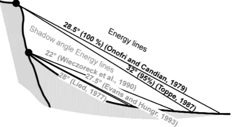
This principle was modified and applied to rockfalls with-out volume dependency using a predefined angle of the line joining the source to the stop point of blocs (φp). φpranges from 22◦ to 37◦ depending on assumptions (Fig. 1a) and based on field evidence (Wieczoreck et al., 1999; Evans and Hungr, 1993; Toppe, 1987; Onofri and Candian, 1979). Such a model can be quickly applied to large areas, where a pre-liminary investigation of the potential rockfall propagation areas is needed starting from known source areas, or for very large rockfalls based on the Heim theory, which is based on the estimation of friction angle depending on volumes.
CONEFALL permits application of this shadow angle principle with grid files DTM that can be used in a geograph-ical information system (GIS). This method can be applied to prioritize detailed investigation based on a global risk analy-sis by crossing objects at risk and potential rockfall areas. 2 Previous work on rockfall trajectory modelling
The principles of rockfall trajectory modelling were stated by Ritchie (1963), who completed experimental studies of rock-fall trajectories, and came up with a classification scheme for rockfall. Rockfall trajectories can be calculated using clas-sical kinematics equations (Piteau and Clayton, 1978; Azimi et al., 1982; Descoeudres and Zimmermann, 1987; Guzzetti et al., 2002). The loss of energy at the impact points is com-monly modelled using coefficients of restitution, which de-pend on a number of factors, including mass, shape, and ve-locity of the boulder. Coefficients of restitution are usually expressed as the ratio of the velocity (or ratio of energy) be-fore and after the impact, eventually for normal and tangen-tial velocity components. Sliding and rolling can be added to the simulation. The blocks are simulated either by points (lumped mass) or rigid bodies. It means that either the tra-jectories depend on the block shapes, or the mass is concen-trated in a point and the influence of shape is given by addi-tional random parameters (Stevens, 1996). For most of the parameters used for the impact calculation, a stochastic part can be added to obtain more realistic results and to reflect the fact that parameters are varying along a slope (Scioldo, 2001; Dudt and Heidenreich, 2001; Guzzetti et al., 2002; Crosta and Agliardi, 2004; Dorren et al., 2006).
It must be noted that observations and modelling in 3 dimensions indicate that the trajectories can be spread around the steepest slopes in a range of±20◦(Agliardi and Crosta, 2003). Modelling has shown that the spreading
in-Fig. 1a. Energy line used for the cone method from the top or the
bottom of a cliff (shadow angle), according to various authors (mo-dified after Crosta et al., 2001).
creases with a smaller DTM grid size, i.e. more accurate (Agliardi and Crosta, 2003). But this can also be achieved by increasing the variability of a DTM altitude of coarser mesh introducing statistical distribution for the altitude variability (Crosta and Agliardi, 2003; Jaboyedoff et al., 2006).
Using GIS, Van Dijke and Van Westen (1990) and Heinimann et al. (1998) as well as Dorren and Seijmonsbergern (2003) simulated rockfall paths starting from source cells and moving to the next one by choosing the nearest neighbouring cell with the lowest elevation. The maximal run-out distance and velocity are computed using an analogy to a sliding coefficient (Scheidegger, 1973). In that case, if a digitized map containing data on the super-ficial geology exists, sliding coefficients can be changed depending on the geological type. Then potential rockfall propagation areas are simulated assuming that the falling rocks follow water flow paths limiting the runout distance by using the energy line, too. This leads to results similar to kinematics modelling (Utelli, 1999). The disadvantage of these methods is that small topographic or morphological irregularities may affect the rockfall trajectory substantially. Men´endez Duarte and Marquinez (2002) used GIS to determine watershed below rockfall sources identified as propagation zones (rockfall basin).
Using the energy line angle (φp), Onofri and Candian (1979) observed that 50% of blocks are stopped for
φp>33.5◦, 72% for φp>32◦, and 100% forφp>28.5◦. Toppe (1987) developed a similar approach for maximum runout distances of snow avalanche and rockfall hazard map-ping using aφpdeduced from the parameters extracted from the fitting of the slope profile by a parabola. Toppe (1987) indicates that 50% of the rockfall boulders are stopped before 45◦and 95% forφ
The energy line angleφpcan also be calculated from the bottom of the cliff or the top of the talus slope, instead of the rockfall source area (Lied, 1977; Hungr and Evans, 1988; Evans and Hungr, 1993) (Fig. 1a). In that case, it is called the shadow angle principle. This assumption can be used when the slope profile contains a slope break creating bolder rebounds where most of the kinetic energy is lost and then it represents a new start of the fall and bounce along the slope (Evans and Hungr, 1993). Lied (1977) found that all the blocks are stopped at an angleφpof 28◦−30◦. The term “shadow angle” is preferably used when the limit is set from the bottom of the cliff, even if the concept of energy line can still be applied because it is assumed that most of the kinetic energy is lost after the first rebound (Jaboyedoff and Labiouse, 2003). Evans and Hungr (1993), using numerous case-studies, set a shadow angle (φp) at 27.5◦. These lim-its are obviously “average” maximum runout points. Sta-tistically, a small percentage of blocks can go beyond the
φp, depending on the slope land cover type. Evans and Hungr (1993) indicate thatφpcan be as low as 24◦, whereas Wieczorek et al. (1999) found a different lower value at 22◦ for the Yosemite valley, in Central California.
3 Theoretical background of CONEFALL
CONEFALL basically uses the principle of Heim (1932), modified and applied to rockfall. Following Heim (1932), the run-out distance (L) of a rock avalanche can be estimated using the intersection of a line connecting the top of the rock-fall scar with a slope equal to tanγ=1z/Lwith the topog-raphy,1zbeing the difference in elevation between the top and the bottom. In the rockfall version the source cliff is re-placed by the location of the rockfall source and the angleγ
is replaced by a fixed limited valueφp(Onofri and Candian, 1979). The energy loss along a complex rockfall trajectory depends on several different mechanisms, but the average of the rockfall energy dissipation can be modelled by friction instead of a punctual loss of energy at impact points, slid-ing and rollslid-ing. This concept can be used because statisti-cally, the energy loss along a slope can be assumed linear on average, which leads in fact to a normal distribution of the block stop point distances around a mean value (Jaboyedoff and Pedrazzini, 2010). This justifies the concept by assum-ing threshold limits for propagation. The energy balance of a rockfall boulder starting from an elevationH is given by (Heim, 1932; Scheidegger, 1973; Evans and Hungr, 1993):
m g H−m g h(x)=1 2m v(x)
2+m g x µ (1)
where:mis the mass of the block,gis gravity acceleration,
x the horizontal coordinate,h(x)the elevation of the topo-graphic surface at point(x,h(x)),v(x)the velocity at point
x, and µthe mean kinetic coefficient of friction (Fig. 1b). Rotational energy is not considered for the sake of simplicity.
Fig. 1b. Variables used to calculate velocities and energies based on
the energy line concept. The example uses the more distant block to defineφpand estimate1h, which is used to calculate the velo-cityv=√2g1h. This illustrates the tailor-made possibilities of the cone method.
Rearranging terms to estimate the stopping point horizontal distancexstop by puttingv(x)=0, and using µ=tgφp, we obtain:
µ=tgφp=
H−h xstop
xstop
(2)
Hence, the boulder stops where the line from the rockfall source area with a slope equal to φp intersects the topo-graphic surface. This line is the energy line. Equation (2) provides a physical meaning toφp, as a mean kinematic co-efficient of friction. From Eq. (1) we can estimate the boulder velocity for any x-position:
v(x)= q
2g H−h(x)−xtgφp
(3) From Eq. (3) it can be seen that ifv(x)is constant, the to-pographic slopeαis equal toφp. Hence, whereα > φpthe boulder accelerates, and whereα < φp, the boulder deceler-ates. Assuming that1his the difference of altitude between the energy line and topography, Eq. (3) can be rearranged to obtain:
1h=v 2(x)
2g (4)
Fig. 2. Relationships between energy line angles and block
distribu-tions according to various authors. The gray curve is a fitting of all results (except the point Toppe, 1987 for 45◦). The obtained value isφp=34◦with a standard deviation of 1.62◦.
As shown above, several authors (see Sect. 2) are giving limits forφp, linked to the percentage of block stopped before this point (Fig. 2). It is important to know if an extreme limit exists. Theoretically the answer is no, because assuming that on average a boulder behaves like a mass sliding along the topography, the distribution of theφpof the block deposition or stopping points is a Gaussian function. Then, if the path is divided into small segments, each of them will have a random value for tanφp, around a mean value. By using the central limit theorem (Jaboyedoff and Pedrazzini, 2010), it can be shown that these random values are distributed according to a Gaussian distribution. In practice,φpvalues of 27◦to 37◦ are usually used for rockfalls, butφpcan be much lower (10– 15◦) in case of rock avalanches.
If all the cells of potential rockfall source areas are used, the angleφpmust be set to a value close to the angle of re-pose of the talus slope: around 36–37◦for De la Noe and De Margerie (1888), 32–38◦ for Evans and Hungr (1993), and ranging from 26◦to 41◦for Jomelli and Francou (2000) (Fig. 1a). Theoretically, 35◦is the upper limit for a pile of
spheres (R´eka et al., 1997). This last value is also very close to one of the most common friction angles in rock mechan-ics. It can be assumed that the highly inclined talus slopes are caused by boulders with special shapes (like bricks that can form vertical walls). When moving down a talus with a slope angle of 35◦, a boulder will keep roughly a constant velocity. Thus, at the bottom of the slope, the block will move beyond the limit defined by the 35◦cone slope to lose its energy completely. Then a slope angle lower than 35◦is necessary to stop the block. Thus, 33–35◦ is a well-based
φplimiting range angle in order to predict the most common distant trajectories of blocks. Moreover, the starting point of the boulder must have a steeper slope than 35◦; otherwise the block will not start to move.
For very large rockfall phenomena, the equation of Scheidegger (1973) may be used to estimateγ.
Fig. 3. Principle of the cone method, with cells as source areas. The
resulting zone is the surface delineated by the higher cone surfaces or envelope of the whole pixels source of individual cones.
4 Cone method implementation
CONEFALL estimates the potential rockfall propagation area using a DTM and a grid file containing all the rockfall source areas as input data. It calculates the rockfall propa-gation area for each rockfall source cell. The routine of de-tecting whether a DTM cell is located below the energy line, i.e. in the propagation area, is equivalent to consider that a cell is located within a cone. This rather simple rule can be implemented by checking if:
1x2+1y2−ctg φp 2
·(H−h(x))2<0 and h(x) < H(5) where1xand1yare the horizontalxandydistances of the DTM point to the source cell (the apex of the cone),h(x)
is the elevation of the cone apex, H is the altitude of the rockfall source point, and (π/2−φp) is the angle of aperture of the cone (Figs. 1b and 3). Note that some non-continuous areas can be obtained by this simple method. They can be avoided using the intersection of these results with a random walk algorithm (Gamma, 2000; Horton et al., 2008).
computed. If the slope dips towards a non-source cell, then the edge-cell is defined as a bottom cliff cell (Fig. 4a, b). If a source area is not a convex polygon or if it contains non-source cells, the algorithm may generate artefacts. To correct inconsistencies produced by this automatic procedure, a tool to correct the source files manually has been implemented (Fig. 4c).
(b) In CONEFALL, the main parameter controlling the propagation is the cone angle which has a fixed value. With-out further indication, the lateral propagation (dispersion) is defined by the intersection of the cone with topography. But the dispersion can also be limited using an azimuth and a tol-erance angle from the source cell. Different types of outputs can be generated by CONEFALL. The main type is a grid containing the zones where rockfall boulders can propagate. In this grid, the value 1 indicates that the cell inside is at least one cone of propagation, and the value –1 indicates that the cell is outside any propagation area.
For each cell of the computed propagation area, it is also possible to count the number of contributing source cells by counting the number of cones including the propagation cell. This yields information on the zones that can be affected by the greatest number of blocks. The output file is then a grid of integer. Note that this counting is strongly dependent on the type of source area used, i.e. border, bottom or entire source area. The best option is to use a complete source area that is an entire cliff in order to get a count representative of the size of the contributing area.
In addition to this, using Eq. (3) CONEFALL can produce maps of maximum or mean velocities and energies, for each cell within the propagation area. A velocity correction factor,
fv, may take a value other than 1. AssumingErot/Etotis the ratio of rotational energy with total kinetic energy, and using Eq. (4), the translation velocityvtcan be expressed by:
vt(x)= s
1−Erot
Etot
2g1h=fv p
2g1h (6)
Assuming that rotational energies represent around 20% of the total kinetic energy of a boulder (Gerber, 1994), fv is then set to 0.9=
√
0.8. This factor can be determined us-ing field observations to obtain a more precise estimation of rock-fall translational velocities. Similar considerations hold for the estimation of rockfall energies, except that a mean block mass must be determined. Mean values of velocities or energies are usually computed using the full source areas. For the maximum values, it is possible to use only the edges of the source areas without changing the final results. Other configurations are left to the preferences of the user.
The CONEFALL software has been written in Microsoft Visual Basic© 6, first under Windows 98 and later on under Windows XP. The program can handle two types of input grid files, ArcGIS (*.ASC) files and Surfer 6.0 (*.GRD) ASCII files (Golden, 2002). DTM and rockfall source areas are pro-vided as grid files and must have both the same geographical
Fig. 4. (a) Illustration of the procedure of border identification. Any
pixel that has a neighbouring point at the locations 1, 2, 3 or 4 with at least one blank pixel (no cliff) is a border. To extract the bottom of the cliff, the space is divided into 3 types of pixels: inside cliff (light grey), border (dark grey) and white outside. (b) To identify a bottom pixel the normal vectorN to the pixel is estimated, and if it is located above its x-y-0 component the pixel is designated as belonging to the bottom of the cliff. (c) Different possibilities for the modification of cliff areas.
coordinates and the same number of rows and columns. The rockfall source cells are coded by integers (0–359◦) and other grid cells must be set to –1. Depending on the type of anal-ysis, the output file contains integer or floating point values. Cells outside the propagation areas have values of –1. Each computer run or project can be saved and loaded (file menu) in a project text file (*.PRC) that contains all the necessary filenames and computation options.
5 Applications
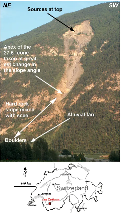
Fig. 5. Les Cretaux location and picture.
steep scree slope containing moved masses and small cliffs. The middle part is a hard rock slope mixed with scree which ends with an alluvial fan, mainly occupied by vineyards. The upper slope gradient is about 40◦, making the use of the
up-per limit of theφpangle (35◦) a good approximation. Lower values ofφpwould represent a more elastic terrain. This im-plies that the lower part slows down the blocks rapidly be-cause of the large plasticity of the soil.
Using all the rockfall source cells, the velocity and en-ergy are computed assuming a rock mass of 3200 kg (corre-sponding to a rock of more than 1 m3). The rockfall volume was selected so that our simulations could be compared to the simulation produced by Jaboyedoff et al. (2005). Fig-ure 6 shows that rockfall blocks are all located within the 35◦ cones. The more distant point is located at 37◦from the top of the cliff. This shows that the 35◦limiting angle is
consis-Fig. 6. The area in black is representing the source cells. The
yel-low to red scale is the count of the number of source points po-tentially contributing to the rockfall propagation zone. The black dashed line indicates the cone taken at the bottom of the source area in black with aφp=27.5◦ and limits equal to 315◦±20◦. The black line indicates the cone taken with an apex taken at the great-est change in the slope angle with aφp=27.5◦. (DTM reproduced with the permission of the Swiss Federal Service of the Topography, BA034918.)
tent with a scree-like topography. In the present case, all the results of the model are identical regardless of whether all the source cells are used or not. The lateral extension of the zone of propagation is larger than the observed spread of rockfall blocks (Fig. 6). However, in comparison to trajectory simu-lations (see Jaboyedoff et al., 2005), the difference of spread is small, but the simulations indicate a maximum run-out dis-tance for a few boulders further than the 35◦slope cones. It must be noted that if the number of contributing source cells in the propagation area is used (Fig. 6), all the boulders are included in the area with more than 45 contributing cones for a total number of 50 source cells. The zone of 50 contribut-ing cones included 30 boulders over a total of 31. This gives a clear indication on the most rockfall-prone area.
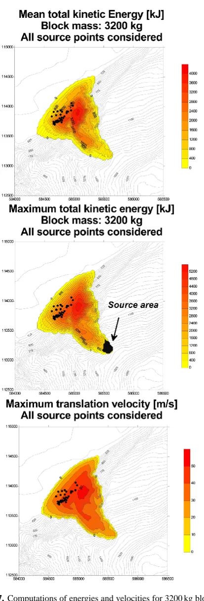
Fig. 7. Computations of energies and velocities for 3200 kg blocks
using the Surfer program. (DTM reproduced with the permission of the Swiss Federal Service of the Topography, BA034918.)
argument, the maximum total kinetic energy is estimated to 3500 kJ, and the maximum mean translational velocity (us-ing a velocity factor = 0.9) is around 42 m s−1(150 km h−1). This is in agreement with the observed maximum translation velocity obtained by Descoeudres (1990) from the analysis of a video record.
Using the “bottom of the cliff” method (Evans and Hungr, 1993) and selecting an angle of 27.5◦, a wider area of pro-pagation is then obtained and is compatible with the extreme boulders simulated with EBOUL (see Fig. 12 in Jaboyed-off et al., 2005) (Fig. 6). To better constrain the potential propagation area, the dispersion is limited by an azimuth and a lateral tolerance angle of 315◦±20◦. The result of the “bottom of the cliff” model appears to be greatly over-estimated. This is because the morphology in our example is not a cliff-slope as in the Rocky Mountains, where Evans and Hungr (1993) developed their method. The 27.5◦area
of propagation compared with 20 000 trajectories simulated by EBOUL (Jaboyedoff et al., 2005) contains 99.8% of the simulated block stoppage points.
Nonetheless, the application of the cone model can also be refined. If we consider that a boulder loses most of its energy at the toe of a cliff or of a channel or at the greatest change in the slope angle corresponding to the apex of the cone com-posed by hard rock and scree slope, aφpangle of 27.5◦can be used by analogy assuming that the apex of the cone is the location of strong energy loss. The computation of a cone centred at this apex shows that all the observed boulders are included in the obtained propagation zone (Fig. 6).
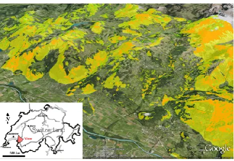
CONEFALL has also been applied at a regional scale to the County de Vaud (Switzerland), a 3200 km2 region. To identify the rockfall source areas, slope angle thresholds (from 47◦to 54◦) were applied according to the local geology and a slope angle histogram analysis (Loye et al., 2009). The
φpangle was set to 33◦ in order to be conservative. In ad-dition, on the plain (significant zone with slope angle below 11◦), the propagation area was limited to stripes of 100 m
along the flank of the valley). The results of this regional study have been shown to be consistent with field observa-tions (Jaboyedoff et al., 2008) (Fig. 8).
6 Discussion and conclusions
Fig. 8. View of rockfall indicative map of the Canton de Vaud based
on the conefall method withφpof 33◦using Googlearth (see Loye et al., 2009 for a detailed description of the map characteristics).
of the energy line angle leads to a cone that defines “lines of energy”.
Nevertheless, the cone method must be applied carefully because the energy line angle varies greatly according to var-ious authors (Fig. 1). In addition, in our experience the re-sults obtained indicate that cones with aφpangle from 33◦to 35◦provide good estimations of propagation zones and
en-ergies in alpine areas. For a high vertical cliff with a scree slope at its toe, the Evans and Hungr method (i.e., “bottom of the cliff or shadow angle approach”) provides better esti-mates of the propagation zones. Further refinements of the cone method require the introduction of energy lines along the flow-paths. This can be performed with algorithms sim-ilar to those used for debris-flows usingD∞flow path and flow dispersion (Holmgren, 1994; Horton et al., 2008; Blahut et al., 2010; Kappes et al., 2011), adding a threshold for the velocity (Horton et al., 2008) or a maximum energy loss from one to another pixel.
Going beyond the previous general statement, the exam-ple of les Cr´etaux shows that energy line angle methods can be applied in several ways with a finer tuning. First, the 50 boulders are included in the 35◦cone centered on the main instability. However, this is not always sufficient to include the extreme run-out blocks. In the simulations performed with EBOUL, 1.75% of the blocks are out of the 35◦energy line angle limit and 0.25% of them propagate further than the 27.5◦limit defined from the top of source area (see
Jaboyed-off et al., 2005). This is consistent with observations consid-ering that only 50 endpoints boulders locations are recorded and that the 27.5◦ limit is very close to the extreme run-out. In addition to using an adapted “bottom of cliff” 27.5◦ method, placing the source at the main slope angle change at the location where the rebounds dissipate the maximum of energy, it is possible to obtain all the observed boulders inside the limit. This example shows that the CONEFALL method can not be applied blindly, the geomorphology and
the goal of a study will directly influence the design of the chosen parameters, i.e. rockfall source areas, bottom of cliff or other morphological arguments. φpmust be then chosen either using previous study or deducing from local field ob-servations.
The CONEFALL method is a good way to get first esti-mations of rockfall “propagation zones”, velocities or ener-gies. At a regional scale the software should be used only as a preliminary mapping tool to delineate rock prone areas using the simple, binary option outlining the areas that can be affected by falling boulders or by counting the number of contributing cones. Continuous variables, such as energy or velocity, should only be used when the morphology has first been inspected carefully to insure correct analysis (selecting among the different possibility of φp angle or the location of the source cells). It must be noted that the shadow angle approach is strongly dependent on the slope morphology. If detailed information are available at regional scale, it is pos-sible to use more sophisticated 3-D models based on trajec-tory modelling (Guzzetti et al., 2003; Crosta and Agliardi, 2004; Frattini et al., 2008; Dorren et al., 2006). For rock avalanches, CONEFALL may be employed using lateral ex-tension, andφpangles calculated by the relationship between
φpangle and the volume after Scheidegger (1973).
Finally, CONEFALL appears to be a suitable standalone solution to perform fast studies of rockfall propagation at re-gional scale, and such a model can be easily implemented in a GIS environment with programming capabilities.
Supplementary material related to this article is available online at:
http://www.nat-hazards-earth-syst-sci.net/11/819/2011/ nhess-11-819-2011-supplement.zip.
Acknowledgements. We thank the Swiss Canton de Vaud regional Authorities and the Cantonal Fire Insurance for financial support within the project CADANAV and for authorizing publication of the results. The first author thanks the Soci´et´e Academique Vaudoise for financial support. An earlier version of the manuscript benefited from the comments of F. Guzzetti from the IRPI Perugia (Italy) and M.-H. Derron from University of Lausanne. One anonymous reviewer, and Luuk Dorren from the Federal Office of Environment of Switzerland and Andreas G¨unther from the Federal Institute for Geosciences and Natural Resources of Germany have greatly improved the manuscript. A. Loye provided one figure for this article. We thank all others for their constructive advice.
Edited by: A. G¨unther
References
Agliardi, F. and Crosta, G.: High resolution three-dimensional nu-merical modelling of rockfalls, Int. J. Rock Mech. Min., 40, 455– 471, doi:10.1016/S1365-1609(03)00021-2, 2003.
Aksoy, H. and Ercanoglu, M.: Determination of the rockfall source in an urban settlement area by using a rule-based fuzzy evaluation, Nat. Hazards Earth Syst. Sci., 6, 941–954, doi:10.5194/nhess-6-941-2006, 2006.
Azimi, C., Desvarreux, P., Giraud, A., and Martin-Coher, J.: M´ethode de calcul de la dynamique des chutes de blocs. Appli-cation `a l’´etude du versant de la montagne de La Pale (Vercors), Bulletin de liaison des Laboratoires des Ponts et Chauss´ees, 122, 93–102(A), 1982 (in French).
Blahut, J., Horton, P., Sterlacchini, S., and Jaboyedoff, M.: De-bris flow hazard modelling on medium scale: Valtellina di Tirano, Italy, Nat. Hazards Earth Syst. Sci., 10, 2379–2390, doi:10.5194/nhess-10-2379-2010, 2010.
Crosta, G. B. and Agliardi, F.: Parametric evaluation of 3D dis-persion of rockfall trajectories, Nat. Hazards Earth Syst. Sci., 4, 583–598, doi:10.5194/nhess-4-583-2004, 2004.
Crosta, G., Frattini, P., and Sterlacchini, S.: Valutazione e gestione del rischio da frana,. RegioneLombardia, Milano, 169 pp., 2001. Corominas, J.: The angle of reach as a mobility index for small and large landslides, Can. Geotech. J., 33, 260–271, doi:10.1023/B:NHAZ.0000007094.74878.d3, 1996.
De la Noe, G. and De Margerie, E.: Du fac¸onnement des versants, in: Les formes du terrain, Imprimerie Nationale, Chapter 3, 39– 47, 1888 (in French).
Descoeudres, F.: L’´eboulement des Crˆetaux. Aspects g´eotechniques et calcul dynamique des chutes de blocs, Publication Soci´et´e Su-isse de M´ecanique des Sols et des Roches, 121, 19–25, 1990 (in French).
Desceoudres, F. and Zimmermann, T.: Three-dimensional dy-namic calculation of rockfalls, in: Proceedings 6th Interna-tional Congress of Rock Mechanics, Montreal, Canada, 337– 342, 1987.
Dorren, L. K. A. and Seijmonsbergen, A. C.: Comparison of three GIS-based models for predicting rockfall runout zones at a regional scale, Geomorphology, 56(1–2), 49–64, doi:10.1016/S0169-555X(03)00045-X, 2003.
Dorren, L. K. A., Berger, F., and Putters, U. S.: Real-size ex-periments and 3-D simulation of rockfall on forested and non-forested slopes, Nat. Hazards Earth Syst. Sci., 6, 145–153, doi:10.5194/nhess-6-145-2006, 2006.
Dudt, J. P. and Heidenreich, B.: Treatment of uncertainty in a three-dimensional numerical simulation model for rockfalls, in: Inter-national Conference on Landslides – causes, impacts and coun-termeasures, edited by: K¨uhne, M., Einstein, H. H., Krauter, E., Klapperich, H., and P¨otter, R., 17–21 June 2001, Davos, Switzer-land, VGE, Essen, 507–514, 2001.
Evans, S. and Hungr, O.: The assessment of rockfall hazard at the base of talus slopes, Can. Geotech. J., 30, 620–636, doi:10.1139/t93-054, 1993.
Frattini, P., Crosta, G., Carrara, A., and Agliardia, F.: Assess-ment of rockfall susceptibility by integrating statistical and physically-based approaches, Geomorphology, 94, 419–437, doi:10.1016/j.geomorph.2006.10.037, 2008.
Gamma, P.: dfwalk-Ein Murgang-Simulationsprogramm zur Gefahrenzonierung, Geographisches Institut der Universit¨at Bern, Switzerland, 2000 (in German).
Gerber, W.: Beurteilung des Prozesses Steinschlag, Forstliche Ar-beitsgruppe Naturgefahren (FAN), Herbstkurs Poschiavo, Kur-sunterlagen, WSL, Birmensdorf, 20 pp., 1994 (in German). Ghazipour, N., Uromeihy, A., Entezam, I., Ansari, F., and Pirouz,
M.: The use of Cone-Fall theory for evaluation of rock-fall haz-ard along the Chaloos-Road (Pol-e-Zanguleh – Marzan-Abad), Geosciences, 17, 160–169, 2008.
Golden: Srurfer version 8.01, Golden software Inc., 2002. Guzzetti, F., Crosta, G., Detti, R., and Agliardi, F.: STONE : a
computer program for the three-dimensional simulation of rock-falls, Computat. Geosci., 28, 1079–1093, doi:10.1016/S0098-3004(02)00025-0, 2002.
Guzzetti, F., Reichenbach, P., and Wieczorek, G. F.: Rockfall haz-ard and risk assessment in the Yosemite Valley, California, USA, Nat. Hazards Earth Syst. Sci., 3, 491–503, doi:10.5194/nhess-3-491-2003, 2003.
Heim, A.: Bergsturz und Menschenleben, Fretz und Wasmuth, Zurich, 218 pp., 1932 (in German).
Heinimann, H. R., Hollenstein, K., Kienholz, H., Krummenacher, B., and Mani, P.: Methoden zur Analyse und Bewertung Von Naturgefahren, Umwelt – Materialen, 85 BUWAL, Switzerland, 247 pp., 1998 (in German).
Hoek, E.: Practical Rock engineering, Rocsciences, available at: http://www.rocscience.com/education/hoeks corner, 313 pp., 2007.
Holmgren, P.: Multiple flow direction algorithms for runoff mod-elling in grid based elevation models: An empirical evaluation, Hydrol. Process., 8, 327–334, doi:10.1002/hyp.3360080405, 1994.
Horton, P., Jaboyedoff, M., and Bardou, E.: Debris flow suscepti-bility mapping at a regional scale, 4th Canadian Conference on Geohazards, Qu´ebec, Canada, May 20–24, 2008.
Hungr, O. and Evans, S. G.: Engineering evaluation of fragmental rockfall hazards, Proceedings 5th International Symposium on Landslides, Lausanne, Switzerland, 1, 685–690, 1988.
Jaboyedoff, M. and Labiouse, V.: Preliminary assessment of rock-fall hazard based on GIS data, in: 10th International Congress on Rock Mechanics ISRM 2003 – Technology roadmap for rock mechanics, South African Institute of Mining and Metallurgy, Johannesburg, South Africa, 575–578, 2003.
Jaboyedoff, M. and Pedrazzini, A.: The usefulness of the reach an-gle concept for hazard zoning using statistical approach. Geo-physical Research Abstracts, Vol. 12, EGU2010-5409, 2010. Jaboyedoff, M., Dudt, J. P., and Labiouse, V.: An attempt to refine
rockfall hazard zoning based on the kinetic energy, frequency and fragmentation degree, Nat. Hazards Earth Syst. Sci., 5, 621–632, doi:10.5194/nhess-5-621-2005, 2005.
Jaboyedoff, M., Giorgis, D., and Riedo, M.: Apports des mod`eles num´eriques d’altitude pour la g´eologie et l’´etude des mouve-ments de versant, Bull. Soc. Vaud. Sc. Nat., 90, 1–21, 2006 (in French).
Jomelli, V. and Francou, B.: Comparing the characteristics of rock-fall talus and snow avalanche landforms in an Alpine environ-ment using a new methodological approach: Massif des Ecrins, French Alps, Geomorphology, 35, 181–192, doi:10.1016/S0169-555X(00)00035-0, 2000.
Kappes, M. S., Malet, J.-P., Remaˆıtre, A., Horton, P., Jaboyedoff, M., and Bell, R.: Assessment of debris-flow susceptibility at medium-scale in the Barcelonnette Basin, France, Nat. Hazards Earth Syst. Sci., 11, 627–641, doi:10.5194/nhess-11-627-2011, 2011.
Labiouse, V. and Desceoudres, F.: Possibilities and difficulties in predicting rockfall trajectories, in: Joint Japan-Swiss seminar on impact load by rockfalls and design of protection structures, Kanazawa, edited by: Masuya, H. and Labiouse, V., 29–36, 1999.
Labiouse, V., Heidenreich, B., Devareux, P., Viktorovitch, M., and Guillemin, P.: Etudes trajectographiques, in: Programme Inter-reg IIc – “Falaises”, Pr´evention des mouvements de versants et des instabilit´es de falaises, Confrontation des m´ethodes d’´etudes des ´eboulements rocheux dans l’arc alpin, edited by: Carere, K., Ratto, S., and Zanolini, F., 155–211, 2001 (in French).
Lan, H., Martin, C. D., and Lim, C. H.: RockFall analyst: a GIS extension for three-dimensional and spatially distributed rockfall hazard modelling, Computat. Geosci., 33, 262–279, 2007. Lied, K.: Rockfall problems in Norway, in: Rockfall dynamics
and protective work effectiveness, ISMES, Bergamo, 90, 51–53, 1977.
Loye, A., Jaboyedoff, M., and Pedrazzini, A.: Identification of po-tential rockfall source areas at a regional scale using a DEM-based geomorphometric analysis, Nat. Hazards Earth Syst. Sci., 9, 1643–1653, doi:10.5194/nhess-9-1643-2009, 2009.
Men´endez Duarte, R. and Marquinez, J.: The influence of en-vironmental and lithologic factors on rockfall at a regional scale: an evaluation using GIS, Geomorphology, 43, 117–136, doi:10.1016/S0169-555X(01)00126-X, 2002.
Onofri, R. and Candian, C.: Indagine sui limiti di massima inva-sione di blocchi rocciosi franati durante il sisma del Friuli del 1976, Reg. Aut. Friuli – Venezia Giulia, Cluet, 42 pp., 1979 (in Italian).
Piteau, D. R. and Clayton, R.: Computer Rockfall Model, Proceed-ings Meeting on Rockfall Dynamics and Protective Works Effec-tiveness, Bergamo, Italy, ISMES, 90, Bergamo, Italy, 123–125, 1978.
R´eka, A., Istan, A., Hornbaker, D., Schiffer, P., and Barabasi, A. L.: Maximum angle of stability in wet and dry spher-ical granular media, Phys. Rev. E, 56, R6271–R6274, doi:10.1103/PhysRevE.56.R6271, 1997.
Ritchie, A. M.: Evaluation of rock-fall and its control, Highway research record, 17, 13–28, 1963.
Rouiller, J. D.: L’´eboulement des cr´etaux – Is´erables – Riddes (Valais), Soc. Suisse de M´ecanique des Sols et des Roches, 121, 15–17, 1990 (in French).
Ruelle, D.: D´eterminisme et pr´edictibilit´e, in: L’ordre et le chaos, Biblioth`eque pour la science, Belin, 136–145, 1987 (in French). Scheidegger, A. E.: On the prediction of the reach and velocity of
catastrophic landslides, Rock Mech., 5, 231–236, 1973. Scioldo, G.: Guide `a l’usage de ISOMAP – INQUIMAP –
RO-TOMAP, Geo & Soft, 66 pp., 2001 (in French).
Spang, R. M.: Protection against rockfall – Stepchild in the design of rock slopes, 6th International Congress on Rock Mechanics, International Society for Rock Mechanics, 551–557, 1987. Stevens, W.: Rockfall 4.0 Software for the Analysis of Falling
Rocks on a Steep Slope, B.A.Sc. thesis, Department of Civil En-gineering, University of Toronto, Ontario, Canada, 1996. Toppe, R.: Terrain models: a tool for natural hazard mapping, in:
Avalanche formation, movement and effects, edited by: Salm, B. and Gubler, H., International, Association of Hydrological Sci-ences, Wallingford, UK, 162, 629–638, 1987.
Utelli, H. H.: Die M¨oglichkeiten von GIS bei der Beurteilung der Steinchlaggefahr im alpinen, Bereich Bull. Angew. Geol., 3–17, 1999 (in German).
Van Dijke, J. J. and Van Westen, C. J.: Rockfall hazard: a geomor-phologic application of neighbourhood analysis with Ilwi, ITC Journal, 1990-1, 40–44, 1990.