R E S E A R C H
Open Access
Finite-size effects in transcript sequencing
count distribution: its power-law correction
necessarily precedes downstream
normalization and comparative analysis
Wing-Cheong Wong
1*, Hong-kiat Ng
2, Erwin Tantoso
1, Richie Soong
2and Frank Eisenhaber
1,3Abstract
Background:Though earlier works on modelling transcript abundance from vertebrates to lower eukaroytes have specifically singled out the Zip’s law, the observed distributions often deviate from a single power-law slope. In hindsight, while power-laws of critical phenomena are derived asymptotically under the conditions of infinite observations, real world observations are finite where the finite-size effects will set in to force a power-law
distribution into an exponential decay and consequently, manifests as a curvature (i.e., varying exponent values) in a log-log plot. If transcript abundance is truly power-law distributed, the varying exponent signifies changing mathematical moments (e.g., mean, variance) and creates heteroskedasticity which compromises statistical rigor in analysis. The impact of this deviation from the asymptotic power-law on sequencing count data has never truly been examined and quantified.
Results:The anecdotal description of transcript abundance being almost Zipf’s law-like distributed can be conceptualized as the imperfect mathematical rendition of the Pareto power-law distribution when subjected to the finite-size effects in the real world; This is regardless of the advancement in sequencing technology since sampling is finite in practice. Our conceptualization agrees well with our empirical analysis of two modern day NGS (Next-generation sequencing) datasets: an in-house generated dilution miRNA study of two gastric cancer cell lines (NUGC3 and AGS) and a publicly available spike-in miRNA data; Firstly, the finite-size effects causes the deviations of sequencing count data from Zipf’s law and issues of reproducibility in sequencing experiments. Secondly, it manifests as heteroskedasticity among experimental replicates to bring about statistical woes. Surprisingly, a straightforward power-law correction that restores the distribution distortion to a single exponent value can dramatically reduce data heteroskedasticity to invoke an instant increase in signal-to-noise ratio by 50% and the statistical/detection sensitivity by as high as 30% regardless of the downstream mapping and normalization methods. Most importantly, the power-law correction improves concordance in significant calls among different normalization methods of a data series averagely by 22%. When presented with a higher sequence depth (4 times difference), the improvement in concordance is asymmetrical (32% for the higher sequencing depth instanceversus 13% for the lower instance) and demonstrates that the simple power-law correction can increase significant detection with higher sequencing depths. Finally, the correction dramatically enhances the statistical conclusions and eludes the metastasis potential of the NUGC3 cell line against AGS of our dilution analysis.
(Continued on next page)
* Correspondence:[email protected]
1Bioinformatics Institute (BII), Agency for Science, Technology and Research
(A*STAR), 30 Biopolis Street, #07-01, Matrix, Singapore 138671, Singapore Full list of author information is available at the end of the article
© The Author(s). 2018Open AccessThis article is distributed under the terms of the Creative Commons Attribution 4.0 International License (http://creativecommons.org/licenses/by/4.0/), which permits unrestricted use, distribution, and reproduction in any medium, provided you give appropriate credit to the original author(s) and the source, provide a link to the Creative Commons license, and indicate if changes were made. The Creative Commons Public Domain Dedication waiver (http://creativecommons.org/publicdomain/zero/1.0/) applies to the data made available in this article, unless otherwise stated. Wonget al. Biology Direct (2018) 13:2
(Continued from previous page)
Conclusions:The finite-size effects due to undersampling generally plagues transcript count data with
reproducibility issues but can be minimized through a simple power-law correction of the count distribution. This distribution correction has direct implication on the biological interpretation of the study and the rigor of the scientific findings.
Reviewers:This article was reviewed by Oliviero Carugo, Thomas Dandekar and Sandor Pongor.
Keywords:Finite-size effects, Nyquist sampling criterion, Aliasing noise, Pareto distribution, Zip’s law, Transcript abundance, Sequencing, Normalization, Heteroskedasticity
Author summary
In the grand scheme of things, the fundamental issue of reproducibility has a long-term implication on scientific rigor in this fast-paced OMICS-frenzy era. Since tech-nology is not always WYSIWYG (What you see is what you get), it is important to validate our observations against some theoretical basis. For transcriptomic ana-lysis, the lack of reproducibility is often hinted by the high discordance among normalization methods in a typical comparative analysis workflow given the same data set. Since important conclusions are often made based on these NGS-derived exploratory results, improv-ing the reproducibility of the sequencimprov-ing outputs be-comes instrumental and ever more so since most bioinformatics analysis seldom bridge the gap between the exploratory finds and the true molecular actuators via the formal arguments of underlying molecular mech-anisms. The latter is especially critical for clinical diag-nostics applications.
Background
Despite some cautionary notes on the generalization of power-law on natural phenomena [1], cell transcript abundance has often been theorized as originating from the family of power-law distributions [2]. Typically visu-alized in terms of histogram or rank-frequency plot, transcript abundance distribution seems to follow the extreme value theory where only a couple of genes are highly-expressed while the rest are relatively lowly-expressed. Earlier works on modelling SAGE-derived (serial analysis of gene expression) transcript abundance from vertebrates to lower eukaroytes have specifically singled out the power-law distribution, namely Zip’s law [3–7] where the slope of a power-law equation is about
−1 on a log-log scale. Originating from information the-ory, this slope describes the ideal compromise between the sender and receiver as the“Principle of Least Effort”; steep line represents a smaller and repetitive vocabulary while a shallower slope represents a larger and more di-verse vocabulary. As such, Zipf statistic evaluates the balance between redundancy and diversity. Remarkably, Zipf’s law seemingly holds for most normal tissues of homogenous cell type and also approximately for the
heterogenous cell type (i.e., the slope tends to be slightly lower than 1.0) [4]. However, there exists a caveat to the power-law association: the observed power-law distribu-tion of transcript abundance is usually imperfect in that it deviates from a single parameterized power-law slope.
By far, it has been unclear if this deviation is either re-flective of the underlying true distribution or indicative of some inherent biases in terms of library size/sequencing depth [8], transcript lengths [9] and GC contents [10] in the physical or technological process that generates the observations. In our best understanding, the implications of the power-law deviation in transcript abundance has never been truly examined in current literature. Presum-ably, most researchers deem this deviation to have min-imal effects on the downstream pre-processing steps like read mapping, normalization and statistical analysis. How-ever, it is clear that there is no general consensus on the pre-processing of RNA-based sequencing data but rather best practices [11], with the normalization step contribut-ing to the largest variation in the workflow performance [12–14].
In retrospect, all power-laws of critical phenomena are derived asymptotically under the conditions of infinite ob-servations. In the real world, observations are finite and, therefore, the deviations from asymptotic power-law is to be expected in finite systems. The latter, which is known as finite-size effects, will force an observed power-law dis-tribution into an exponential decay and presents itself as a curvature in the log-log plot [15]. Pertaining to the nature system that governs the cell transcript abundance, the crit-ical question is to clarify if the observed power-law devi-ation is truly the result of the finite-size effects and not because the underlying distribution cannot be simply de-scribed by power-law [16,17].
variance to the data and poses additional difficulty to normalization methods where a good method aims to reduce variance without increasing bias [18]. Secondly, heteroskedasticity will bias test statistics since Type I and Type II error increases with underestimated and overestimated standard errors respectively as a conse-quence of unequal variance [19,20].
In this work, we derived a generalized concept whereby the anecdotal description that transcript abundance se-quencing count data is almost Zipf’s law-like distributed can now be objectively quantified by the Pareto power-law distribution via its mathematical moments and how the distribution can be rendered mathematically imperfect when subjected to the finite-size effects in the real world; a manifestation of the aliasing noise when undersampling occurs. Our formalism concurs well with our empirical analysis of two modern day NGS (Next-generation sequen-cing) datasets: an in-house generated dilution miRNA study of two gastric cancer cell lines (NUGC3 and AGS) and a publicly available spike-in miRNA data; Firstly, the finite-size effects causes deviations of sequencing count data from Zipf’s law and the issues of reproducibility is-sues in sequencing experiments that seems inescapable despite the advancement in sequencing technology since sampling is finite in the real world. Secondly, finite-size ef-fects manifests as heteroskedasticity among experimental replicates to create statistical woes.
Collectively, this justifies for a simple restoration of the sequencing count data towards a power-law distribu-tion with a single exponent value, herein as power-law correction, to reduce sample variance of lower transcript counts towards homoskedasticity for improved statistical outcomes. When this method was evaluated in a typical NGS comparative analysis workflow that entails (i) read mapping/count quantification (ii) pre-filtering of the zero counts across conditions (iii) normalization and (iv) the statistical testing, the signal-to-noise ratio (SNR) of the workflow improved by 50% after power-law correc-tion. In turn, this higher SNR translates to an increase in statistical and detection sensitivity by approximately 30% in the dilution analysis regardless of the mapping and normalization methods used in the evaluation. Most im-portantly, the power-law correction addresses a long-standing issue of discordance in the comparative analysis workflow, particularly attributed to the variations among different normalization methods [12–14]. Using the dilu-tion study, the increase in concordance rate was aver-agely 22% from the baseline rate of (48.24 ± 7.07)% to (70.32 ± 6.72)% upon power-law correction. When a higher sequencing depth is presented, power-law correc-tion can extract the addicorrec-tional informacorrec-tion content to increase significant detection. Specifically, in the dilution analysis, the higher sequencing depth instance (by four times higher) has an increase concordance rate of 32%
(44.6% ± 4.91% versus 76.25% ± 1.78%) while it was 13% (51.88% ± 7.26% versus 64.39% ± 3.65%) for the lower depth instance. Finally, power-law correction statistically enhances the biological context of the experiment and elu-cidates the multiple metastatic signatures of the NUGC3 cell line in the dilution study of two gastric cell lines.
Results and discussion
Finite-size effects introduces curvature in sequencing count data distributions, impacts the reproducibility of the experiment and brings about heteroskedasticity among experimental replicates
Two miRNA sequencing datasets composed of technical replicates were being examined; The choice of miRNA is deliberate to avoid both transcript length bias [9] and abundance quantification [21] as confounding factors. The first miRNA set is the background count data of a spike-in experiment from a published study (GEO data-set: GSE67074) that contains 12 replicates [11]; The original authors’ BWA-mapped counts were used. The second set is an in-house generated dilution series of two gastric cancer cell lines - AGS and NUGC3 (See methods for details: The dilution dataset [22]). In this section, only the Bowtie1-mapped NUGC3 set of 8 tech-nical replicates that spans across 4 concentration points of 12pM, 6pM, 3pM and 1.5pM was used. The varying concentration design aims to simulate the different se-quencing depth (i.e., the total mapped reads) that mimics a system of various sizes to study its finite-size effects (SeeAdditional file1: Figure S1).
Given that these datasets are made up of replicates, a simple intra-sample scaling where the counts of each replicate is divided by the maximum count of the same transcript within the replicate, will suffice. Furthermore, instead of visualizing Zipf’s law distribution with rank-frequency graphs, the Pareto distribution plots were used (See methods for details: Transformation between rank-frequency and Pareto distribution). This has the added advantage of characterizing the sequencing count data with the mathematical moments (i.e., mean, stand-ard deviations) of the Pareto’s density function that is lacking in a typical Zip’s law plot.
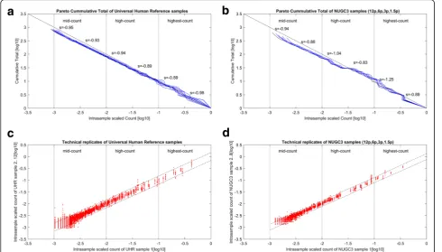
Figure1aandbdepict the cumulative histograms, spe-cifically the Pareto distribution plots of the scaled counts from the spike-in background and NUGC3 dilution dataset (See methods for details: Property of Type I Pa-reto distribution). The plots are segmented into its ap-propriate highest-count to lowest-count linear ranges based on an order of magnitude per segment (see verti-cal dotted lines across horizontal axis). In both cases, the highest-count segments approach the Zipf’s law (see dashed black line) which has a characteristic slope of−1. Beyond that, the slope values generally decreased and fin-ished with an inflection for the lowest-count segments.
While there is a general convergence of slope values from the highest-count to the mid-count segments, a specific divergence for the low and lowest-count seg-ments can be readily seen. In the case of the dilution set, its divergence is more exaggerated (as marked by the split-end pattern) as a consequence of a more de-liberate sequencing depth differences among the repli-cates. The latter marks the effects of the finite-size effects which plays a major role in the reproducibility of the observed distributions.
Meanwhile, the trend towards changing slopes along the count segments indicates a general deviation from a single power-law exponent. Based on the mathematical moments of the Pareto distribution (Eqs. 3 and 4), expo-nent values of below“1”indicates asymptotically infinite moments. The consequence of these infinite moments is that their empirical estimates can converge very slowly due to the frequent occurrences of extreme values [23]. When coupled with the changing exponents along the count segments, heteroskedasticity (i.e., unequal error variance) among the replicates can be expected from the imperfect power-law distributions.
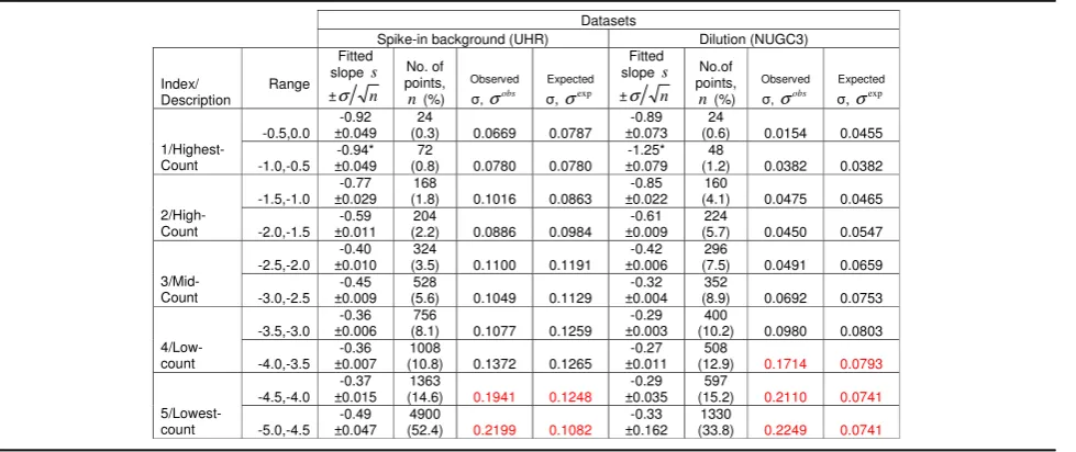
To further emphasize, the scatterplots of the scaled counts for the 11 replicates of the spike-in background set against the replicate with the highest total reads were examined in Fig. 1c. Concurrently, Fig. 1d depicts the scaled count of the 7 NUGC3 replicates of the dilution set against the NUGC3 12pM sample with the highest total reads. Similar segmented ranges are also superim-posed on these figures. Complementing Fig. 1c and d, the regression slope of the power-law fit, the total num-ber of points, the observed and expected standard devi-ation of each segmented range were computed and complied in Table1. Of particular importance is the ex-pected standard deviation which projects the exex-pected heteroskedasticity of the replicate noise across the count segments. It is extrapolated from the observed standard deviation of a reference count segment after accounting for the slope differences between the reference segment and the other segments (See Table 1 legend for further explanation).
Essentially, the observed heteroskedasticity seen in the Fig.1cand dexhibits the hallmark of the Pareto’s math-ematical moments where a change in variance is
perpetuated by a change in the power-law exponent. Furthermore, the observed heteroskedasticity can be di-vided into variances of reproducible (i.e., the degree of agreement between experimental results conducted by different individuals/locations/instruments) and irrepro-ducible origin. Specifically, when heteroskedasticity is about equal between the observed (i.e., general spread of the datapoints) and the expected (i.e., margins marked by the dotted lines at 99% confidence interval) standard deviations, it is simply reflective of the reproducible rep-licate noise as for the cases of the highest to mid-count segments. However, when heteroskedasticity spreads be-yond the expected margins, it indicates additional irre-producible noise as for the cases of the diverged low and lowest-count segments. In the worst cases, the observed standard deviation exceeds that of the expected by about 2 times for the spike-in background set and 3 times for the NUGC3 dilution set (SeeTable1: values in red).
The irreproducible noise that plagued the diverging low and lowest-count segments, serves to highlight the instability of the replicated count values when the corre-sponding power-law mathematical moments stem not only from low exponent values but of non-comparable magnitude as well. The latter basically demonstrates the impact of the finite-size effects on the same physical sys-tem when sampled at different rates. Since irreproduc-ibility can occur even for a set of replicates that has similar sequencing depths like the case of the spike-in set, it is expected to be worse for any datasets that have more diverse depths as attested by the dilution set.
Unfortunately, none of the commonly used normalization methods namely DESeq [24,25], Relative Log Expression (RLE) [24, 26], Trimmed Mean of M-values (TMM) [26, 27], UpperQuartile (UQ) [12,26], Count Per Million (CPM) [26] and Quantile [18, 28]) can correct for the power-law deviations in both datasets; Both power-law de-viation and heteroskedasticity remain (SeeAdditional files 2: Figure S2 and Additional files3: Figure S3).
Aliasing noise explains the finite-size effects that distorts the theoretical power-law distribution of sequencing count data
In fact, the sequencing procedure can be recast into a sampling problem: The total transcript population in a cell can be viewed as a library of unique transcript spe-cies with different frequency of occurrences. Simply put, this library can be thought as the composites of a con-tinuous analogue signal. And when this analogue signal is subjected to sequencing, it undergoes a sampling pro-cedure where the abundance of the individual transcript species in terms of its counts, is being quantified. Col-lectively, the digitized counts becomes the sampled sig-nal of the origisig-nal asig-nalogue sigsig-nal.
Mathematically, a power-law type sampled signal Y(f) with an amplitude of So and an exponent of α, can be described as the sum of its original signal Sof−α and its alias term So(fs−f)−α given any frequencyf (see Eq. 13) and can be visualized as a frequency-domain plot. With any sampling procedure, undersampling will occur when
Table 1Summary of analysis for spike-in background and NUGC3 dilution datasets
The summarized analysis for two datasets, namely the spike-in background and dilution datasets, were presented. The spike-in set consists of 1387 transcripts over 12 replicates while the dilution set has 865 transcripts over 8 replicates. For each segmented range, the fitted slope to Pareto distribution, the total number of points, the observed and expected standard deviation are calculated. The expected standard deviationσexp
gives the corrected standard deviation of each“slope < 1”segment as if its slope is the same as the reference segment (indicated by *). It is calculated via the formulaσexp
segi¼σ
obs
segrefðssegref=ssegiÞusing the
highest-count segment as the reference. For the spike-in set, the observed and expected standard deviation is about 2 times larger while this is about 3 times for the dilution set (highlighted in red) in the worst case
the Nyquist sampling criterion of fmax< 2fs is not satis-fied where fmax is the largest frequency component of
the original signal andfsis the sampling frequency. As a consequence, this will result in a non-zero alias term
So(fs−f)−α. More specifically, the condition of aliasing where a distortion of the sampled signal Y(f) from its original signal will occur [29] (See methods for details:
Derivation of the alias term in the power-law 1/
fαequation; Eqs. 5-13).
In relation to the sampled signal Y(f), the rank vari-able y and maximum count value C1 of the
rank-frequency equation (see Eq. 14) are analogous to the frequencyfand the amplitudeSoofY(f) respectively. In turn, the rank-frequency and Pareto’s tail distribution are inversely related to each other (See methods for details: Transformation between rank-frequency and Pareto distribution; Eqs. 14-17). Essentially, the Pareto plots can be straightforwardly transformed into a frequency-domain plot.
To determine if undersampling has occurred, the sam-pling frequencyfs needs to be first determined between the sampled signal and its original signal to check if the Nyquist sampling criterion is fulfilled. The best estimate or surrogate of the original signalSof−αcan be estimated from the replicate with the largest total reads within the data series. For the dilution set, this was one of the 12p NUGC3 sample which consists of a total of 632 unique count values. In the case of the spike-in background set, the replicate with the largest total reads has 863 unique count values. Corresponding to their rank-frequency (frequency-amplitude) plots, this translate to a maximum rank (frequency) of 632 and 863 accordingly.
Using the respective surrogates as baseline, the ob-served alias noise between a sampled signal and its ori-ginal signal can be then determined by taking their logarithmic differences as described by the mathematical expression logΔY(f) = log[Sof−α+So(fs−f)−α]−log[Sof−α] (see Eq. 19). Since Zip’s law (see eq. 14 where b= 1) holds for the high and highest-count segments of both data-sets, the exponent term is implicitly set to α= 1. Alias noiseΔY(f) reaches its maximum whenf=fmaxsuch that ΔY(f) =ΔY(fmax), for which the sampling frequency fs can be solved by evaluating logΔY(fmax) (See methods for
details: Solving for sampling frequency fsto determine
undersampling; Eqs. 18–21).
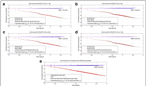
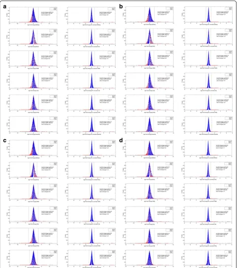
Furthering the analysis of the scaled datasets in Fig.1, Fig. 2 shows the rank-frequency plots for the NUGC3 dilution and the spike-in replicates (marked in red). In particular, Fig. 2a–eshow the plots for the 1.5p pair, 3p pair, 6p pair, single 12p replicate and the 11 UHR repli-cates against the best estimate of the original signals (marked in black). In addition, the observed alias noise (marked in blue), together with the corresponding
theoretical alias noise So(fs−f)−α (marked in magenta), are shown in the sub-figures. For each case, the sam-pling frequencyfsand the mean square error (MSE is
de-fined as the residual error between the observed and theoretical alias noise) are given as well. The overall low MSE values of between 5.67e-4 to 3.58e-3 indicates a good fit between the theoretical alias noise model and the observed alias datapoints.
Within the NUGC3 dilution set, the 1.5pM, 3pM, 6pM replicates have failed to satisfy the Nyquist sam-pling criterion of fmax< 2fs at sampling frequencies of 589, 592 and 1045 (See Fig.2a–c) respectively. Since the minimum sampling frequency needed by the NUGC3 di-lution set is 1264 (2 × 632), undersampling has occurred for these cases. Undersampling can also be concluded for the spike-in background dataset at a sampling fre-quency of 1464 (See Fig. 2e) where the required mini-mum sampling frequency is 1726 (2 × 863). In contrast, only the single 12pM case had satisfied the Nyquist cri-terion atfmax< 3.4fs(SeeFig.2d). Theoretically, the sam-pling frequency for a zero alias noise tends to infinity (solve eq. 17 forΔY(fmax) = 1at f=fmax).
In hindsight, the finite-size effects has always plagued sequencing-based studies since the early days [7] where the alias noise manifests as the misfitted tail in Zipf’s law distributions. The magnitude of the finite-size effects is dependent on the severity of undersampling and it can now be quantified formally through a simple recasting of the Pareto plot to the frequency-domain plot.
The necessity of power-law correction on sequencing count data to restore distribution distortion
With larger slope values than before, it implies that the standard deviation for all count segments, should theoretically converge towards a smaller value. Indeed, Fig. 3c and d of the respective data sets show that the corrected count values exhibit less heteroskedasticity across all count segments and variation among the repli-cates. This reduced heteroskedasticity is to be expected if transcript abundance is power-law distributed and ad-heres to its mathematical moments (see Eqs. 3 and 4); In hindsight, it does indeed. Furthermore, based on Table2 (markings in red), the difference between the observed and expected standard deviation is merely 1.1 times for the spike-in background dataset and 1.6 times for the NUGC3 dilution dataset in the worst case. The stark improvement from before the power-law correction (i.e., worst case of 2 times and 3 times respectively) signifies that the irreproducible noise in the data series has been dramatically reduced in the form of alias noise. Overall, it translates to a smaller dynamic range for the corrected values where the uncorrected count values from the low
and lowest-count segment have now been shifted to the mid-count segment.
When the corrected spike-in background and NUGC3 dilution data sets were subjected to a re-analysis of aliasing, the corrected datasets shows a general absence of undersampling. The rank-frequency plots for the cor-rected dilution replicates are depicted by Fig. 4afor the 1.5p pair, Fig. 4bfor the 3p pair, Fig. 4cfor the 6p pair and Fig. 4d for the single 12p, while Fig. 4e shows the corrected spike-in background replicates for the set of 12 UHR replicates (marked in red). The best estimate of the original signal is marked by black in each figure. The corresponding observed alias noise (marked in blue), as well as the theoretical alias noise So(fs−f)−α (marked in magenta), shows very slight aliasing in all cases given their new sampling frequencies of 1720, 1311, 1783, 3315 and 1920 respectively. The overall low MSE values of between 6.00e-4 to 1.87e-3 indicates a good fit between the theoretical model and the observed alias.
Fig. 2Rank-frequency plots of NUGC3 dilution and spike-in background datasets.a,b,c,dandeshow the rank-frequency plots for the 1.5p pair, 3p pair, 6p pair, single 12p replicate and the 11 UHR replicates against the best estimate of the original signals (marked in black). Meanwhile, the observed alias noise (marked in blue) and the theoretical alias noiseSo(fs−f)−α(marked in magenta), are also shown. In each subplot, the sampling
frequencyfsand the mean square error (MSE is defined as the residual error between the observed and theoretical alias noise) are given as well.
Overall, the low MSE values of between 5.67e-4 to 3.58e-3 indicates a good fit between the theoretical alias noise model and the observed alias datapoints. For the NUGC3 dilution set, the 1.5p, 3p, 6p replicates have failed to satisfy the Nyquist sampling criterion offmax< 2fsat sampling
frequencies of 589, 592 and 1045; Undersampling has occurred for these cases. The same can also be concluded for the spike-in background dataset. Only the single 12p case had satisfied the Nyquist criterion atfmax< 3.4fs
Fig. 3Post power-law correction, Pareto distributions and scatterplots of spike-in background and dilution datasets.aandbgive the Pareto distribution plots of the scaled background counts from the spike-in background and NUGC3 dilution dataset respectively, after the power-law correction was applied. Both plots are segmented into the highest-count to lowest-count regions based on an order of magnitude per segment (see vertical dotted lines across horizontal axis). Both plots display a power-law distribution with a more uniform slope throughout all count segments. In fact, the power-law correction estimates how the true underlying distribution should have been without aliasing. Meanwhile,canddshow that the corrected count values exhibit less heteroskedasticity across all count segments and variation among the replicates with the increase in slope values after the power-law correction. Finally, the minimum count value of each replicate has increased such that the uncorrected count values previously (SeeFig.2CandD) in the low and lowest-count segment have now been moved into the mid-count segment
Table 2Summary of analysis for the power-law corrected spike-in background and NUGC3 dilution datasets
The summarized analysis of the Zipf’s law corrected datasets, namely the spike-in background and dilution datasets, were presented. The spike-in set consists of 1387 transcripts over 12 replicates while the dilution set has 865 transcripts over 8 replicates. For each segmented range, the fitted slope to Pareto distribution, the total number of points, the observed and expected standard deviation are calculated. The expected standard deviationσexp
gives the corrected standard deviation of each“slope < 1”segment as if its slope is the same as the reference segment (indicated by *). It is calculated via the formulaσexp
segi¼σ
obs segrefðssegref=
ssegiÞusing the highest-count segment as the reference. For the spike-in set, the observed and expected standard deviation is about 1.1 times larger while this is
Power-law correction should precede normalization; it increases signal-to-noise ratio and sensitivity of statistical testing/detection in comparative analysis
To rigorously evaluate the impact on power-law correc-tion in a typical NGS comparative analysis workflow, Fig. 5 shows the evaluation setup that permutes across 4 mapping algorithms (Bowtie1, Bowtie2(global) [30], Novoalign (www.novocraft.com) and BWA [31,32]) and 6 normalization methods (DESeq [24, 25], Relative Log Expression (RLE) [24, 26], Trimmed Mean of M-values (TMM) [26, 27], UpperQuartile (UQ) [12, 26], Count Per Million (CPM) [26] and Quantile normalization
[18, 28]). Furthermore, the comparisons were split into the positive (signal between NUGC3 and AGS samples) and the negative (noise within the NUGC3 replicates) tests. For the statistical analysis, the generalized linear model [33] from the EdgeR package [26] was used for the multiple contrasts where each comparison pro-duced a set of fold-change values, average counts (in terms of counts-per-million) and p-values (See methods for details: Generalized NGS comparative analysis).
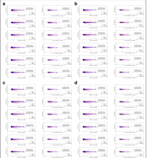
Figure 6a shows the MA-plots (i,e., average count
versus fold-change) of the Bowtie1-mapped dilution dataset before (left-column) and after (right-column) the power-law correction for the 6 normalization algorithms (arranged in row-wise). This Bowtie1-mapped set com-prises of 637 paired AGS-NUGC3 paired-transcripts. Likewise, Fig. 6b–ddepict the MA-plots of the Bowtie2 (global), Novoalign and BWA-mapped dilution analysis where the total amount of mapped transcripts are 657, 673 and 670 respectively. Their respective PPS settings was referenced from the Bowtie1-mapped set’s optimum setting to standardize the parameter settings of the power-law correction step across the mapping algorithms (See methods for details: Computation procedures for power-law correction of a count data set).
For each MA-plot, the positive signal is depicted in red while the noise is shown in blue. The noise model, as a simple linear regression of y=mx, attempts is depicted dotted line. For both signal and noise data-points, their corresponding residual with respect to the fitted noise model gives the fold-change variation along
Fig. 4Post power-law correction, rank-frequency plots of NUGC3 dilution and spike-in background datasets.a,b,c,dandeshow the rank-frequency plots for the 1.5p pair, 3p pair, 6p pair, single 12p replicate and the 11 UHR replicates against the best estimate of the original signals (marked in black) after the power-law correction. The observed alias noise (marked in blue) and the theoretical alias noiseSo(fs−f)−α(marked in
magenta), are also shown. In each subplot, the sampling frequencyfsand the mean square error (MSE is defined as the residual error between the
observed and theoretical alias noise) are given as well. The overall low MSE values of between 6.00e-4 to 1.87e-3 indicates a good fit between the theoretical model and the observed alias. Generally speaking, the corrected datasets shows a general absence of undersampling. For all plots, the observed alias noise (marked in blue), as well as the theoretical alias noiseSo(fs−f)−α(marked in magenta), shows very slight aliasing in all cases
given their new sampling frequencies of 1720, 1311, 1783, 3315 and 1920 respectively
the average count axis (or x-axis) and can be recapitu-lated into a summary statistics. Essentially, the summary statistics gives the amount of bias (the mean) and vari-ance (the standard deviation) of the normalization method where an effective one should reduce variance without increasing bias [18]. Furthermore, signal-to-noise ratio (SNR) of each mapping/normalization pair, defined as Eðx2
signalÞ=σ2noise where Eðx2signalÞ is the expect-ation of the second moment of the signal and σ2
noise is the variance of the noise, was also computed. For each mapping algorithm, the median measures of the signal residual, noise residual and SNR across all normalization methods are also taken and summarized in Table 3 (see
Additional file4: Table S1 for full details).
Throughout all the MA-plots, heteroskedasticity in the noise comparisons (depicted in blue) can be readily seen without the power-law correction. Heteroskedasticity brings about two issues: Firstly, it introduces both bias and large variance to the comparisons as attested by the mean and standard deviation ranges of −0.192 to − 0.153 and 2.189 to 2.229 for the positive comparisons (or signal) (Table 3 column 3). In contrast, this was
between 0.001 to 0.006 and between 1.017 to 1.022 for power-law corrected analysis (Table 3 column 6). Over-all, the correction improved the SNR by about 50% (i.e., 17–11/11) given the SNR of the corrected and uncor-rected analysis at about 17 times and 11 times respect-ively (Table3columns 4 and 7).
Secondly, heteroskedasticity, which manifests as un-equal variance, can bias the test-statistics where Type I and Type II error will increase with underestimated and overestimated standard errors respectively [19]. To further emphasize, Fig.7a–d show the same Bowtie1, Bowtie2(-global), Novoalign and BWA-mapped dilution analysis in terms of their volcano plots (i.e., log fold-changesversus p-values). Likewise, the left and right columns show the be-fore and after power-law correction for the 6 normalization algorithms (arranged in row-wise).
In each volcano plot, the noise comparisons can essen-tially be treated as the null hypothesis. As such, the log fold-change and p-value cutoffs (marked by double hori-zontal dotted lines and single vertical dotted line) for the purpose of deriving the significant number of transcripts in the positive comparisons, were determined from the largest absolute fold-change value and smallest p-value of these 6 noise comparisons (in blue). The latter aims to exclude any false-positives. Furthermore, the rate of change in p-value against fold-change can also be derived from the two cutoff values and is indicated in each vol-cano plot. Finally, for each of the 4 positive comparisons, the exact breakdown of the number of significant tran-scripts for all combinations of mapping and normalization methods before and after power-law correction were com-puted (see Additional file5: Table S2 for full details).
Based on the volcano plots, the slower rate of change in p-values of the uncorrected cases when compared to the power-law corrected cases, implies that a higher fold-change threshold is required to achieve a compar-able p-value (or Type I error rate) during statistical test-ing. Consequently, the higher fold-change threshold also implies a larger type II error (i.e., failing to detect an ef-fect that is present) for the uncorrected cases and hence, a compromised sensitivity on the statistical testing. In-deed, based on Table 4, the general number of signifi-cant transcripts are higher for the power-law corrected analysis than the uncorrected ones. The trend is consist-ent regardless of the mapping algorithms used when averaged over the 6 normalization methods for each posi-tive comparison. Meanwhile, it should also be noted that the variation contributed by different normalization algo-rithms is larger than that of different mapping methods. Overall, the average increase in sensitivity (in terms of per-centage) across the 4 comparisons after power-law correc-tion, is between 26% to 28% (36~ 42 transcripts versus 50~ 57 transcripts) for the Bowtie1-mapped analysis, be-tween 27% to 30% (41~ 44 transcripts versus 58~ 61
Fig. 6MA-plots of dilution data set before and after power-law correction. Fig.6shows the MA-plots (i.,e., average countsversusfold-changes) of the dilution dataset before (left-column) and after (right-column) the power-law correction. In particular, Figsa,b,canddshows the MA-plot analysis for 4 mapping (Bowtie1, Bowtie2(global), Novoalign and BWA) algorithms while the permutation of the 6 normalization algorithms (DESeq, Relative Log Expression (RLE), Trimmed Mean of M-values (TMM), UpperQuartile (UQ), Count Per Million (CPM) and Quantile normalization) are arranged in a row-wise manner. For the power-law correction, the optimum PPS setting was evaluated to be 55 (SeeAdditional file6: Fig. S5A). In each MA-plot, the positive and noise signal are shown in red and blue respectively. The noise model (y=mx) is shown in dotted lines; Ideally, the slope value is 0 for no bias. The signal and noise residuals with respect to the noise model give the fold-change variation along the average count axis (or x-axis). Overall, it is apparent that the heteroskedasticity (see left-column) of the uncorrected AGS and NUGC3 count values has propagated down to the level of comparative analysis regardless of any combination of mapping and normalization methods. However when power-law correction is applied, heteroskedasticity was dramatically minimized (see right-column)
transcripts) for the Bowtie2(global)-mapped analysis, be-tween 26% to 34% (36~ 43 transcripts versus 54~ 58 tran-scripts) for the Novoalign-mapped analysis and between 26% to 32% (36~ 41 transcripts versus 53~ 58 transcripts) for the BWA-mapped analysis.
Independent validation of power-law application on the full spike-in data series
As an independent validation, the full spike-in dataset which includes the 12 non-human spike-in transcripts was also analyzed. Given 12 samples in total without technical replicates across conditions, the total number of possible pairwise comparisons is 66 cases (C122 ) where the positive set is made up of the 12 spike-in transcripts (or signal) while the negative set (or noise) is composed of 460 UHR transcripts after filtering for non-zero count values among the conditions. In addition, given that the original authors’ BWA-mapped counts were used, the permutation step across the 4 mapping algorithms was excluded. Also, due to the cyclic latin-square design of the spike-in transcripts across the 12 samples, the uniqueness of each sample meant that there are no repli-cates and hence, statistical evaluation is not possible. In-stead, the cutoff criteria for significant call is simply based on the fold-change. As an additional note, the optimum PPS setting for the power-law corrected data was evaluated to be 10 according to the optimization plot (SeeAdditional file6: Figure S5B). Note that due to the lack of replicates for the spike-in transcripts, only the background set was used for the parameter estimation.
Figure 8 shows the receivers operator characteristics (ROC) curves for the 6 normalization methods: DESeq, Relative Log Expression (RLE), Trimmed Mean of M-values (TMM), UpperQuartile (UQ), Count Per Million (CPM) and Quantile normalization. For each ROC plot, the sensitivity and specificity values were derived through the permutation of the log fold-change range of the noise comparisons. The plot without correction is shown in red
while the power-law corrected one is depicted in blue. From the ROC plots, there is an obvious improvement in the performance across all tested normalization methods after the power-law correction. Among the methods, the performance is almost comparable to one another with the exception of the quantile normalization method. Fur-thermore, to compare against the BWA performance of the dilution analysis, the sensitivity of the spike-in analysis for each normalization method was evaluated at the false-positive rate of 0 (See the sensitivity values before and after power-law correction in the ROC plots). As compared to the improvement in statistical sensitivity of 26% to 32% in the dilution analysis, the improvement in detection sensi-tivity for the spike-in analysis is lower (i.e., between 15% to 17%) across all the methods since its undersampling con-dition was less severe than that of the dilution data set.
Power-law correction improves the concordance in significant transcript call among normalization
algorithms, especially with increased sequencing depth
Another important implication of the power-law correction is that the improved concordance in significant transcript call among the different normalization methods [12–14] will decrease the workflow’s dependency on the variations in specific algorithms. Returning to the dilution data set analysis, Table 5 gives the average concordance in sig-nificant calls by various mapping/normalization methods (seeAdditional file5: Table S2 for the detail breakdown). It summarizes the level of agreement between the 6 normalization algorithms per mapping method for the positive comparisons in NGS workflow as shown in Fig.5. Briefly, the“intersect”row gives the total number of com-mon significant transcripts with the same fold-change dir-ectionality among the 6 algorithms, the “union” row gives the total number of significant transcripts reported by any of the 6 algorithms while the concordance ratio (in %) is taken between the “intersect” total and the “union” total. The concordance ratio serves as an unbiased measure given its double-edged sword nature; While an increase in signifi-cant call by all algorithms is necessary to increase the
Table 3The average signal-to-noise characteristics of the comparative dilution analysis (AGS versus NUGC3) before and after power-law correction
Original data Power-law corrected data
Mapping method Median residual (μ±σ)noise
Median residual (μ±σ)signal
Median
signal-to-noise ratioEðx 2
signalÞ
σ2
noise
Median residual (μ±σ)noise
Median residual (μ±σ)signal
Median
signal-to-noise ratioEðx 2
signalÞ
σ2
noise
Bowtie1 0.018 ± 0.649 −0.192 ± 2.229 11.3 0.002 ± 0.261 0.006 ± 1.021 15.4
Bowtie2 (global) 0.019 ± 0.642 −0.169 ± 2.200 11.3 0.002 ± 0.244 0.003 ± 1.022 17.6
Novoalign 0.017 ± 0.641 −0.153 ± 2.189 11.3 0.001 ± 0.238 −0.001 ± 1.017 18.2
BWA 0.017 ± 0.648 −0.159 ± 2.193 11.1 0.001 ± 0.242 0.001 ± 1.019 17.8
Fig. 7Volcano plots of dilution data set before and after power-law correction. Akin to Fig.6, the volcano plots of the dilution dataset before (left-column) and after (right-column) the power-law correction is shown in Fig.7. In particular, Figsa,b,canddshows the MA-plot analysis for 4 mapping (Bowtie1, Bowtie2(global), Novoalign and BWA) algorithms while the permutation of the 6 normalization algorithms (DESeq, Relative Log Expression (RLE), Trimmed Mean of M-values (TMM), UpperQuartile (UQ), Count Per Million (CPM) and Quantile normalization) are arranged in a row-wise manner. Overall, the apparent asymmetrical spread of the noise comparisons (in blue) of the uncorrected data set demonstrates the non-zero fold-change bias despite the application of various normalization methods. Most importantly, the slower rate of change inp-values of the uncorrected cases (see left-column) when compared to the power-law corrected cases (see right-column), implies that a higher fold-change threshold is needed to acquire the same p-value (or Type I error rate) during statistical testing. In turn, a higher fold-change threshold also implies a larger type II error (i.e., failing to detect an effect that is present) for the uncorrected cases and eventually, a compromised sensitivity on the statistical testing
“intersect” count, it also increases the likelihood that only some of the algorithms are making the call, thus lowering the concordance ratio.
With the power-law correction, the increase in the “intersect” total has almost doubled for all mapping/ normalization combinations across all comparisons (see
“intersect”rows). Meanwhile, the corresponding increase in the“union” total is less than one-quarter at its worst (see“union”rows). This gives an increase of about 22%
in concordance rate after the power-law correction i.e., (70.32 ± 6.72)% versus (48.24 ± 7.07)% (See “ sum-mary statistics” first row in Table 5). When the com-parisons are further stratified by their sequencing depths (i.e., AGS-12p and AGS-3p comparisons), an increase in sequencing depth does not necessarily improve the con-cordance rates. In fact, the higher sequencing depth AGS-12p instance has a lower concordance rate of (44.6 ± 4.91)% than that of the lower sequencing instance at
Table 4Median number of significant transcripts calls in the comparative dilution analysis (AGS versus NUGC3) before and after power-law correction
Original data Power-law corrected data
Mapping method AGS 12p vs NUGC3 12p
AGS 12p vs NUGC3 3p
AGS 3p vs NUGC3 12p
AGS 3p vs NUGC3 3p
AGS 12p vs NUGC3 12p
AGS 12p vs NUGC3 3p
AGS 3p vs NUGC3 12p
AGS 3p vs NUGC3 3p
Bowtie1 42 41 39 36 57 52 52 50
Bowtie2 (global) 44 43 43 41 61 59 61 58
Novoalign 43 40 39 36 58 57 57 54
BWA 41 41 39 36 58 55 56 53
The breakdown of significant transcript calls for each combination of the mapping algorithms (Bowtie1, Bowtie2(global), Novoalign and BWA) and normalization methods (DESeq, RLE, TMM, Upperquartile, CPM and Quantile) for all 4 positive comparisons (AGS-12pversusNUGC-12p, AGS-12pversusNUGC-3p, AGS-3pversus
NUGC-12p and AGS-3pversusNUGC-3p) are given in the following table. The median number of significant calls for 6 normalization methods are highlighted in red for each mapping algorithm
(51.88 ± 7.26)% (See “summary statistics” second row in
Table5). In retrospect, although the number of significant transcript calls or the “intersect” total has generally increased with a higher sequencing depth, the incon-sistency in significant transcript calls among the various normalization methods (i.e., the “union” total) has in-creased at a faster rate which resulted in a lower concord-ance rate despite the higher sequencing depth.
With the power-law correction, a higher sequencing depth correctly returns a higher concordance rate. Be-tween the uncorrected and power-law corrected analysis, the improvement is somewhat asymmetrical where it was about 32% (44.6% ± 4.91% versus 76.25% ± 1.78%) for the higher sequencing depth AGS-12p instance while this was about 13% (51.88% ± 7.26% versus 64.39% ± 3.65%) for the lower depth AGS-3p instance. It remains that sufficient sequencing depth is necessary to generate enough infor-mation but when the condition is met, power-law correc-tion will be able to extract any addicorrec-tional informacorrec-tion content to increase significant detection.
Enhanced statistical conclusions elucidates the metastatic potential of the NUGC3 gastric cancer cell line
While both AGS and NUGC3 cell lines were commonly described as gastric adenocarcinoma according to the Cellosaurus database (version 22; http://web.expasy.org/
cellosaurus/), NUGC3 was derived from a distal
metasta-sis site - the Brachialis muscle of a male patient and AGS is presumably taken from the primary site of a fe-male patient. Therefore, their comparison should elude the metastasis potential of the NUGC3 cell line beyond the common gastric adenocarcinoma. According to current
literature, the common metastasis site of stomach cancer (in ascending order) is the liver, peritoneum, lung and bone [34,35] while it is considerably rare to spread to the pan-creas and skeletal muscle [36,37]. When compared to gen-eric adenocarcinoma which often spreads to the liver and lung [38], signet-ring adenocarcinoma frequently metasta-sizes within the peritoneum, bone, ovaries and sometimes to the breast [34,39].
In our comparative study of the two gastric cell lines, the Bowtie1-mapped concordance transcripts from Table 5 before and after power-law correction were independently subjected to gene-set enrichment analysis (GSEA) via the MiEAA webserver to identify plausible disease groups from the collection of Hu-man microRNA and Disease Database (HMDD). Briefly, using the Bowtie1-mapped results from Table 5, the concordance transcripts across the 4 comparisons be-fore power-law correction (see“intersect row”; columns 3– 6) were compiled into a union set of concordance tran-scripts. The same was done for the power-law corrected comparisons (see “intersect row”; columns 7–10). Altogether, the uncorrected and power-law corrected union sets consist of 30 and 52 concordance pre-cursor miRNA transcripts respectively (see Additional file 7: Table S3 columns 1 and 2). The uncorrected list exceeded the maximum intersect value of 28 (AGS-12p versus
NUGC3–12p) due to some slight variations among the 4 comparisons. Between the two concordance sets, the un-corrected set is almost a complete subset of the un-corrected set; one transcript is unique to the uncorrected set while this was 23 for the corrected set (SeeAdditional file7: Table S3 columns 3 and 4).
Table 5Concordance summary of significant transcripts calls of comparative dilution analysis (AGS versus NUGC3) before and after power-law correction
The following table gives the agreement of significant transcript calls among the 6 normalization methods (DESeq, RLE, TMM, Upperquartile, CPM and Quantile) for each mapping algorithms (Bowtie1, Bowtie2(global), Novoalign and BWA) for the following 4 positive comparisons: AGS-12p versus NUGC-12p, AGS-12p versus NUGC-3p, AGS-3p versus NUGC-12p and AGS-3p versus NUGC-3p. The summary statistics row gives the concordance of comparisons (i) across all sequencing depth (top row) and (ii) stratified by sequencing depth (bottom row)
Thereafter, both lists were independently subjected to gene-set enrichment analysis (GSEA) via the MiEAA webserver to identify plausible disease groups from the collection of Human microRNA and Disease Database (HMDD). For the power-law corrected list, the specific parameters are as follows: count≥10 and FDR-adjusted
p ≤0.05; This gives a maximum expected value of 0.5 for false-positives (FP). To match the FP count of 0.5,
the necessary parameters for the uncorrected list are: count≥5 and FDR-adjusted p ≤0.1 (See Table 6 legend for detailed explanation).
Table 6 consolidates the identified HMDD categories of both analysis sorted by observed count, then by FDR-adjusted pvalue. The expected baseline category -“adenocarcinoma” was used as the cutoff point for signifi-cance and hence, any categories beyond it were considered
Table 6miRNA enrichment of concordance transcripts before and after power-law correction
as insignificant hits (marked in black). Within the significant categories, there are two likely false-positive hits (marked in blue). They are the “Leukemia, Myeloid, Acute” hit that should be grouped with the non-significant “Leukemia, Lymphocytic, Chronic” and the “Carcinoma, Squamous Cell”hit that should group with the non-significant“ Esopha-geal Neoplasms”hit to explain esophageal cancer.
Between the uncorrected and power-law corrected re-sult sets, the latter presents the stronger evidence of ex-pected gastric adenocarcinoma through its more significant p-values for both “stomach neoplasms” and “adenocarcinoma”. Likewise, the remaining significant hits suggest several neoplasms and carcinoma (“lung neoplasms”, “pancreatic neoplasm”, “ovarian neoplasm”
“carcinoma, non-small-cell lung”) as possible metastasis sites for NUGC3 with stronger statistical conclusions being drawn from power-law corrected analysis. In addition, power-law analysis discovers two more metas-tasis categories - “carcinoma, hepatocellular” and “breast neoplasms” with significant p-values 0.015 and 0.023 respectively. Overall, the power-law corrected analysis concurs significantly better with the clinical evidence.
Conclusion
Specifically, our work has identified and mathematically quantified an important technical limitation of the se-quencing technology for transcriptomics applications where finite-size effects due to undersampling [15, 29] can have profound effects on the reproducibility and statistical qualities of underlying transcript abun-dance distribution for its subsequent interpretation; This is independent of the advancement in sequen-cing technology since sampling is finite in the real world. With a simple distribution correction, the signal-to-noise ratio and sensitivity of statistical detec-tion in a typical comparative analysis can experience an instant and dramatic improvement that greatly impacts the reliability of the final biological interpretation of the study.
Methods
Property of type I Pareto distribution
When transcript abundance is being visualized in a rank-frequency plot, the Zip’s law [3–7] is specifically being sin-gled out. Meanwhile, there exists a close relationship be-tween the family of Pareto distributions (Type I, II, II and IV) to the Zip’s law; Type II to IV Pareto distributions var-ied from Type I mainly from the addition of a location and shape parameter that are irrelevant to the modelling of transcript abundance. Among the Pareto family, the Type I Pareto distribution remains the most mathematic-ally compatible to the rank-frequency plot where their two axis can be shown to be interchangeable (See methods for
details: Transformation between rank-frequency and Pa-reto distribution).
Mathematically, the probability (PDF) and cumulative (CDF) density function of the Type I Pareto distribution are defined as:
P Xð ¼x;xmin;sÞ ¼
sxs min
xsþ1 ð1Þ
P Xð ≤x;xmin;sÞ ¼
1− xmin x
s
for x≥xmin
0 for x<xmin
8 <
: ð2Þ
for the intervalx≥xminandxminis the minimum value of
the distribution and is necessarily positive (i.e.xmin> 0). In
addition, the Pareto’s tail distribution (complementary CDF) is simply defined as P(X>x). Correspondingly, the mean and variance of the Pareto distribution are given as:
μ¼
sxmin
s−1 for s>1
∞ for s≤1
8 <
: ð3Þ
σ2¼
sx2 min
s−1
ð Þ2
s−2
ð Þ for s>2
∞ for 0<s≤2
8 > < >
: ð4Þ
Therefore, for large values of the exponent terms, the corresponding mean μ and variance term σ2 converges towards smaller values for a fixedxmin.
Derivation of the alias term in the power-law 1/fαequation
Aliasing refers to a distortion or an artifact when a re-constructed signal differs from its original continuous signal. In this section, the alias term for the power-law equation 1/fα is derived. Note that the main derivation originates from Kirchner [29] and this section provides only a concise adaptation.
Given a time series x(t), its Fourier transform of its discrete sampled time seriesy(t) is given as:
Y fð Þ ¼
Z∞
−∞
x tð ÞIII tð Þe−i2Πftdt ð5Þ
Furthermore, given that the sampling function III(t) is a periodic function at a sampling interval of Δt= 1/fs, it can be defined as:
III tð Þ ¼X
∞
−∞
ckei2Πkfst ð6Þ
whereck¼Δ1t RΔt=2
−Δt=2∂ðfstÞe−i2Πkfstdt¼Δ1t
1
fs¼1 for all k.
Combining Eqs. (5) and (6), one can re-express the Fourier transform ofy(t) into:
Y fð Þ ¼
Z∞
−∞
X∞
k¼−∞
ei2Πkfstx tð Þe−i2Πfstdt
¼ Z∞
−∞
X∞
k¼−∞
x tð Þe−i2Πðf−kfsÞtdt ð7Þ
Also, given that the summation is taken over all k, the term−kfscan replace bykfs. Together with interchanging the summation and integration sign, one yields the following:
Y fð Þ ¼ X
∞
k¼−∞
Z∞
−∞
x tð Þe−i2ΠðfþkfsÞtdt
¼ X∞
k¼−∞
X fð þkfsÞ ð8Þ
In addition, the sampled functionY(f) can be decom-posed into its original signal X(f) and its alias compo-nents as follows:
Y fð Þ ¼X fð Þ þ X
∞
k¼−∞;k≠0
X fð þkfsÞ ð9Þ
Sincex(t) is a real function, its Fourier transformX(f) is Hermitian. Therefore,X(−f) =X(f) and Eq. (9) can be written for positive frequencies only as follows:
Y fð Þ ¼X fð Þ þX
∞
k¼1
X kfð s−fÞ þX kfð sþfÞ ð10Þ
Substituting the power-law equation X(f) =Sof−α into (10) yields:
Y fð Þ ¼Sof−αþ
X∞
k¼1
Soðkfs−fÞ
−α
þX∞
k¼1
SoðkfsþfÞ−α ð11Þ
For Eq. (11) to converge mathematically, (i) the high frequency component (kfs+f) cannot be ex-tended infinitely; In real-world, high frequency com-ponents fall off faster than 1/fα way above the sampling frequency) and (ii) the condition where
α> 1 needs to be satisfied. Hence, the Fourier trans-form of x(t) can be simplified to the following form:
Y fð Þ ¼Sof−αþ
X∞
k¼1
Soðkfs−fÞ−α ð12Þ
Furthermore, for a band-limited signal of 0≤f≤fmax, the
only relevant alias term is (fs−fmax) wherek= 1, since (kfs−
fmax) > 0 will satisfy the Nyquist sampling criterion offmax<
kfsfor whichk≥2. In other words, aliasing will not occur for
k≥2. Finally, the power-law Fourier series ofx(t) with the relevant alias term when undersampling occurs, is given as:
Y fð Þ ¼Sof−αþSoðfs−fÞ
−α ð
13Þ
whereY(f) is the sampled function,Sof−αis the original signal andSo(fs−f)−αis the alias component.
Transformation between rank-frequency and Pareto (type I) distribution
The Pareto (Type I to IV) distribution belongs to the large family of power-law distributions; the subsequent deriv-ation refers specifically to the Type I Pareto distribution. Given an observation, the Pareto’s tail distribution ( comple-mentary CDF) describes how many cases are seen greater than the observation in terms of cumulative density func-tion (CDF). Meanwhile, the rank-frequency distribufunc-tion is an inverse CDF (quantile function) seen in a reverse order with respect to the Pareto distribution, where it depicts the occurrence of the observation at a given rank.
First, let the rank-frequency equation be defined as:
x¼C1y−b ð14Þ
where y is a yth ranked value and x is the number of observed occurrences at y. One can further implies that there exists y number of values for which their corre-sponding x values are greater than C1y−b. As such, one
can write a cumulative density function for random vari-ableX for the number of observations larger thanC1y−b
in the form:
P X>C1y−b
¼C2y ð15Þ
where C2is a normalization constant such thatP(X≥
C1y−b)≤1 must be satisfied. Then, rearranging Eq. (14)
into y¼ ½x C1
−1
b and substituting it into Eq. (15) yields the Pareto’s tail distribution or complementary CDF:
P Xð >xÞ ¼C2
x C1
−1
b
ð16Þ
¼ ½ x xmin
−1
b for x≥x
min. Meanwhile, to convert from the
complementary CDF to the complementary cumulative total function (CTF), the expression can simply be rear-ranged as follows:
y¼ 1 C2
P Xð >xÞ ¼C−1b
1x− 1
b ð17Þ
Hence, comparing terms in Eqs. (14) and (17), it can be seen that the Pareto’s tail distribution (in terms of complementary CTF) and rank-frequency distribution are inversely related.
Solving for sampling frequencyfsto determine undersampling
Taking logarithm on both sides of Eq. (13), the sampled functionY(f) can be rewritten in logarithmic form as:
logY fð Þ ¼ log½Sof−α
þ log Sof
−αþS oðfs−fÞ
−α
Sof−α
ð18Þ
The second term on the right hand-side gives a distor-tion ratio between an aliased signal Sof−α+So(fs−f)−α and original signalSof−α. As such, let the distortion ratio
ΔY(f) be defined as:
ΔY fð Þ ¼Sof
−αþS
oðfs−fÞ−α
Sof−α ð
19Þ
Further simplification yields:
ΔY fð Þ ¼1þðfs−fÞ
−α
f−α ð20Þ
And solving for the sampling frequencyfsgives:
fs¼ f þf ½ΔY fð Þ−1−1α ð21Þ
For a rank-frequency plot where Zipf’s law holds (i.e., α= 1), fs can directly be evaluated when f=fmax, ΔY(f)
=ΔY(fmax).
Derivation of the power-law correction factor
In an earlier section, the rank-frequency distribution and Pareto’s tail distribution has been proven to be inversely related to each other. For the purpose of es-timating the exponent term in the rank-frequency plot, a better approach is to use Pareto’s tail distribu-tion. This is because the large-ranked tail of rank-frequency distribution tend to be clustered with small
values of the same rank. As a result, this give a hori-zontal tail. In contrast, the same segment is always monotonically-increasing in Pareto. As such, let the count and rank of the ith transcript be x and y re-spectively. Then the rank-frequency equation in its Pareto’s tail distribution form or complementary CTF can be written as.
y¼kx−s ð22Þ
where y=C2⋅P(X≥x), k¼C−1s and s¼1b from Eq. (17).
Taking logarithm on both sides, the expression is re-written as:
logby¼ logbkþmlogbx ð23Þ
where the slope and intercept are represented by m=
−s and logbk respectively. Then, to convert the original slope and intercept (m, logbk) to a reference set of pa-rameters (mref, logbkref), we let:
logby¼ logbk−logbkref
þ logbkref
þmref
m mref
logbx
logby¼ logbkrefþ logb
k kref
xmref m mref
! ð24Þ
In the original scale, the rank-frequency equation can be re-expressed as:
y¼kref
k kref 1 mref x m mref
" #mref
ð25Þ
Finally, the corrected countx'is given as:
x0¼ k kref
1
mref x
m
mref ð26Þ
The power-law correction is implemented in PERL language and can be downloaded from the supplemen-tary website [22].
Computation procedures for power-law correction of a count data set
The restoration of an observed distribution towards an uniform power-law entails that the slopes of all count segments to be the same. The reference power-law slope is taken from the highest-count segment since this seg-ment is sampled from the higher abundance transcripts
and should have the best mathematical convergence to-wards its real value. And with the correction toto-wards a common slope, it is expected that all count segments will have similar variation among the replicates and that the overall heteroskedasticity should be dramatically reduced. Without the loss of generality, the proposed sequencing count correction will be, herein, named as the power-law correction.
In the actual implementation of the power-law correc-tion procedure, there are two important computacorrec-tional aspects to note. Firstly, for the purpose of estimating the exponent term in a rank-frequency plot, the Pareto equa-tion (see Eq. 21) is used rather than Zipf’s (see Eq. 14) be-cause the large-ranked tail of Zipf’s law tends to be clustered with small values of the same rank. As a result, this gives a horizontal tail which is sub-optimal for slope estimation. In contrast, the same segment is always mono-tonically increasing in Pareto.
Secondly, the power-law correction is performed at a per-sample level. The total number of count segments in a Pareto plot is dependent on a fixed number of points per segment, herein, as points-per-segment (PPS). The partitioning of points will start from the highest count value. For each partitioned count segment, a set of slope and intercept (m, logbk) values will be solved using linear regression (see Eq. 22). The first-fitted count segment of the replicate which mimics the highest-count segment, will be used as the reference set of slope and intercept (mref, logbkref) values for the subsequent power-law cor-rection via Eq. 26.
To find the optimum PPS setting that will yield the best overall fit between any replicate to a reference repli-cate in a N-sample dataset, the PPS parameter first needs to be permuted across a range of between 5 to 100 at an interval of 5. At a given PPS setting, two mea-sures can be derived. First, the median of the N first-fitted count segment slopes of the data series can be taken. Secondly, a total of (N-1) R2(i.e., coefficient of de-termination) values can be derived from the linear re-gression results between the N-1 replicates against the reference replicate. Consequently, a median R2can also be taken.
The preceding computational procedures were then applied to the original BWA-mapped spike-in back-ground and Bowtie1-mapped NUGC3 dilution data. Additional file 8: Figure S4A and S4B show the median slope of the first-fitted segments versus the median R2 value of the spike-in background set and the NUGC3 di-lution set respectively. The PPS values are indicated be-sides the data points in the plots. Like before, the reference replicate was taken as the replicate with the largest total reads within the data series for the neces-sary R2computations. For both Figures, the refined solu-tion space of the optimum PPS is indicated by the error
margins defined by the slope of the first highest-count segments from Table 1. Within this margin, the optimum PPS value is determined by the largest median R2 value. As such, the optimum PPS settings for the spike-in background set and the NUGC3 dilution set are 20 and 45 respectively. The subsequent analysis is then based on the power-law corrected data sets using these PPS settings and their associated median slopes as the reference slope values for the respective data series. Similarly, the procedures were also applied to the BWA-mapped spike-in and Bowtie1-BWA-mapped full dilution data sets to obtain the optimum parameters (see Additional file 6: Figure S5A and S5B). The parameter sets were subsequently used on the Bowtie2(global)-mapped, Novoalign-mapped and BWA-mapped full dilution data sets to generate the results in Table3.
The dilution dataset
Overview of design: The dilution series was created for two gastric cancer cell lines - AGS and NUGC3. The NUGC3 set consists of 8 replicates and spans across 4 concentration points of 12p, 6p, 3p and 1.5p so that each concentration contains exactly two technical replicates. Meanwhile, the AGS set is similarly designed except that it consists of 4 replicates across 2 concentrations of 12p and 3p. The varying concentration design aims to simu-late the different sequencing depth (i.e., the total mapped reads) that mimics a system of various sizes to study its finite-size effects. The original sequencing files (in FASTQ format) of this dilution dataset can be down-loaded from the supplementary website [22].
≥8000 g. Column is transferred to a new collection tube and spin at≥8000 g for 5 min at room temperature to re-move residual ethanol and total RNA elute in 10ul of RNase-free water.
TruSeq small RNA library construction and sequencing: 6 (4 for NUGC3 and 2 for AGS) small RNA libraries were prepared in parallel for both NUGC3 and AGS cell lines using the Illumina TruSeq small RNA sample preparation kit according to manufacturer’s instruction. The 6 samples were uniquely indexed to enable sequencing of all 6 librar-ies in one MiSeq flow cell. Briefly, 1μg of total RNA was li-gated with 5′and 3′adapter, cDNA was converted with SuperScript II Reverse Transcriptase and RT Primer. The cDNA was PCR amplified for 12 cycles with RNA PCR Primer and unique PCR Primer Index provided; It is im-portant to note that indexing during PCR amplification minimizes the issue of barcoding bias [40] which masks significant expression differences between miRNA librar-ies. Amplified cDNA construct were first purified using QIagen MinElute PCR Purification kit and the construct were then size selected for fragments ranging between 145 bp to 150 bp using 10% TBE PAGE Gel. The indexed libraries were quantified individually by qPCR using KAPA SYBR FAST qPCR Kit (Kapa Biosciences, inc). To stimulate differences in sequencing depth in a multiplex sequencing experiment, the small RNA libraries for the NUGC3 cell line were pooled such that there was a 1, 2, 4 and 8× difference in concentration between the four unique libraries (12pM, 6pM, 3pM, 1.5pM). Small RNA li-braries for AGS was pooled such that there is a 4× differ-ence in concentration between the two unique libraries (12pM and 3pM). The libraries from both cell lines were pooled to yield a single pooled library and sequenced twice on the MiSeq instrument using MiSeq Reagent v2 for 1 × 40 + 6 (index) sequencing cycle (Illumina Inc., CA, USA).
Generalized NGS comparative workflow
Read mapping:
Raw data in FASTQ format was preprocessed using Trimmomatic [41] version 0.33 by trimming adapter sequences, removing trailing or leading low quality bases (base quality below 3). Subsequently, scan the reads with a 4-base wide sliding window and trim when the average base quality drops below 15. Specif-ically, the command for Trimmomatic is:
The preprocessed reads were then aligned to miRBase v21 primary sequences using three different aligners, i.e. Bowtie (version 1.1.1 and 2.3.0) [30], Novoalign (www.novocraft.com; version V3.04.06) and BWA (version 0.7.12-r1039) [31,32] with the specific parameters as shown below:
Aligned reads in BAM format is then quantified using BEDtools [42] by counting how many reads map to each of the miRNA transcript. The respective mapped count files can be downloaded from the supplementary website [22].
For normalization, the EdgeR, DESeq and preprocessCore R packages were used in this work. Prior to normalization, the data is first organized into its specific cell lines (NUGC3, AGS) and concentration (12pM, 6pM, 3pM, 1.5pM) groups of 2 technical replicates via the following command:
Next, the data is read from an input file to perform the specific normalization. At the same time, an EdgeR DGE-list object and the associated normalization factors for the proper scaling of the raw library sizes will also be created.
For DESeq normalization, the combined commands are as follows:
For Quantile normalization, the combined commands are as follows:
For CPM normalization, the combined commands are as follows:
For TMM, RLE, upperquartile normalization where m takes one of the following values “TMM”,“RLE”,“ upper-quartile”, the commands are as follows:
For performing statistical analysis, the generalized linear model (GLM) [33] from the EdgeR package was used. First, the count data is first fitted to the negative binomial model in the EdgeR package [26] for the purpose of