Stepwise haplotype analysis:
Are LD patterns repeatable?
A.P. Mander
1* and A. Bansal
21MRC Human Nutrition Research, Elsie Widdowson Laboratory, 120 Fulbourn Road, Cambridge, CB1 9NL, UK 2GlaxoSmithKline, New Frontiers Science Park, Harlow, Essex, CM19 5AW, UK
*Correspondence to: Tel:þ44 (0)1223 426356; Fax:þ44 (0)1223 437515; E-mail: [email protected]
Date received (in revised form): 9th November 2005
Abstract
A variety of techniques exist to describe and depict patterns of pairwise linkage disequilibrium (LD). In the current paper, a new log-linear framework is proposed for the summarisation of local interactions among single nucleotide polymorphisms (SNPs). Our approach provides a straightforward means of capturing the diversity of higher-order LD relationships for small numbers of loci by investigating inter-marker interactions. Our method was applied to a dataset of 76 SNP markers spanning a genomic interval of length 2.8 megabases. The analysis of three short sub-regions is described in detail here. Model and graphical representations of contiguous markers in medium to high LD are presented. In the regions studied, evidence for sub-structure was detected, supporting the view that the genomic reality is complex. Interestingly, a critical evaluation of the method by bootstrapping showed that while some LD relationships were captured in a highly repeatable fashion, the majority were not. Large numbers of small interactions, both direct and indirect, mean that many models can adequately summarise the data at hand. Our results suggest that repeatability should be further investigated in the application of LD-based approaches.
Keywords:haplotype blocks, linkage disequilibrium, SNPs, log-linear models, EM algorithm
Introduction
The abundance of single nucleotide polymorphisms (SNPs) and the limited power, in some situations, of single-locus analysis has led to increased use of haplotype-inference methods such as Clark’s algorithm,1the Expectation-Maximisation (EM) algorithm2and iterative-sampling algorithms to resolve phase ambiguity by both coalescent and non-coalescent models.3,4
Recent studies5 – 9have shown that the human genome can be viewed in terms of haplotype blocks, given by discrete regions of high linkage disequilibrium (LD), and separated by shorter regions of low LD. Haplotype block identification has been conducted via evaluation of measures of LD, such as Lewontin’s D’, as well as by methods of directly assessing evidence of recombination.10The corollary of the block concept was that a small proportion of the SNPs, the ‘haplo-type-tagging’ SNPs, should be sufficient to capture the majority of the haplotype structure contained in blocks genome-wide.11More recently, Bayesian graphical modelling has been applied to describe more complex patterns of relationship, for example among loci that are proximal but non-adjacent.12
We introduce a novel application of log-linear modelling, to describe higher-order interactions among SNPs. The log-linear
step is embedded within the EM algorithm in order correctly to model phase. Previously, log-linear models have been used to form the basis of Bayesian priors in resolving phase and to model different levels of LD with known phase.13,14 We show that the log-linear model may be used to describe discrete islands of LD,15as well as smaller conditionally independent sub-fragments of high LD. We test the repeatability of our findings by bootstrapping and find instances of complex LD for which model repeatability is low.
Materials and methods
The methods described below were applied to a dataset con-sisting of a random sample of 150 Caucasian controls from the Prevention of REStenosis with Tranilast and its Outcomes (PRESTO) study.16,17Appropriate consent was obtained and these samples were genotyped across 76 SNPs spanning approximately 2.8 megabases (Mb), within and around the
UGT1A1gene. These data and their analyses are described in detail elsewhere.18
EM log-linear approach
Our method takes as its basis the EM algorithm.2In summary, log-linear modelling is used in the E-step to update haplotype
frequencies, while the likelihood of the data, given the model, is maximised in the M-step. The process proceeds iteratively.
More formally,3given a sample of ndiploid individuals from a population, letG¼(G1,. . ., Gn) denote the known genotypes, letH¼(H1,. . ., Hn)denote the unknown corre-sponding haplotype pairs and let F¼(F1,. . ., Fm)be the unknown population haplotype frequencies. The algorithm starts under random assignment of genotypes. The M-step of the EM algorithm then finds the set of haplotype frequencies,
F,which maximises the following likelihood:
LðFÞ ¼PrðGjFÞ ¼Yn
i¼1
PrðGijFÞ:
Under Hardy–Weinberg equilibrium, the genotype probabilities can be partitioned into the product of haplotype probabilities:
PrðGijFÞ ¼
ðh1;h2Þ[Vi X
Fh1Fh2
whereViis the set of all (ordered) haplotype pairs consistent with the multilocus genotypeGi.
The E-step of the algorithm, used here, then estimates the population haplotype frequenciesF by using the log-linear model and not the traditional counting method. Investigation of the saturated log-linear model, however, in which all loci and interactions are represented, is challenging due to the necessarily high number of parameters. Therefore, a stepwise approach of fitting intermediate models has been used. These intermediate models contain more parameters than a model of complete linkage equilibrium (LE) but fewer parameters than the saturated model.19,20In the current paper, we show how such models provide the framework for quantifying the patterns of LD.
Notation
Notation for the remainder of the paper will focus on the composition of the log-linear model, as it is this that is of interest in describing patterns of SNP interaction. The variable corresponding to theith SNP is given byliand models are specified by using the Wilkinson and Rogers notation, where the SNP variables are combined by ‘þ’ to denote independence, and ‘*’ to denote interaction.21For example, l1þl2denotes independence between the first and second SNP andl3*l4denotes interaction between the 3rd and 4th.
Forward stepwise algorithm
We propose a forward stepwise approach to determining a parsimonious model of LD. Starting with a model of complete LE, higher-order LD terms are added sequentially to the model until a parsimonious model is found. This procedure has been implemented as the commandswblockwithin STATA22 and is available using thessccommand. A likelihood ratio test
(LRT) was used to measure the strength of LD or inter-SNP interaction, although other test statistics are possible. The LRT was performed usinghapipf, a command20implemented in STATA.22
More formally, the algorithm examines a region ofnSNPs. In order to preserve efficiency of the EM algorithm, fewer than ten SNPs is practical. The first step is to estimate the log-likelihood under the base model of LE l1þl2þ. . .þln. Then, every pairwise SNP interaction term is added to this model and the LRT, comparing the new model with the base model is re-evaluated. The most significant interaction term is then added to the base model, this becomes the new base model and the process repeats. A nominalp-value of 0.05 was initially chosen to compare new models with the base model; however, other thresholds ofp¼0.01 andp¼0.001 were also investigated. Once no more pairwise interactions are significant, the algorithm proceeds to the next order of inter-action terms, and so on. This approach accommodates the fact that pairwise interactions can occur over greater distances than contiguous pairs and that LD does not decay monotonically with distance. At each step, the number of degrees of freedom is minimised in the sequence of LRTs, and the algorithm con-tinues until the highest interaction term is evaluated.
Application to LD structure
Certain LD features have been helpfully described in a review by Wall and Pritchard,23who established three criteria, derived using pairwise LD, for assessing haplotype blocks. They introduced concepts of ‘holes’ and ‘overlapping blocks’ in regions of high LD, and these concepts are applicable to more general evaluations of complex LD structure. As described below, these concepts can be presented in terms of log-linear models.
Holes arise when the outermost SNPs are not in strong LD with an SNP or multiple SNPs that lie in between. To translate this to a log-linear framework, consider a triplet of markers parameterised as ll, l2andl3. If l1and l3show high LD, but intervening pairs (l1,l2and l2,l3) do not show high LD, as can happen with low frequency SNPs, then this situation may be described by the modell1*l3þl2.
This representation can be extended to a fourth SNP,l4, in a similar fashion. Continuing the example of a hole at SNP2 (variablel2), one model describing the interactions would bel1*l3*l4þl2. Alternatively, if the three-way interaction is not needed, then another suitable model might be
l1*l3þl3*l4þl1*l4þl2, where, again, SNP2 (l2) is independent of the other three SNPs.
In reality, there may be a combination of holes and overlap-ping regions. The method may be easily generalised.
Investigating the repeatability of derived
models
Regression approaches are better suited to hypothesis generation than to inference, due to the large number of models evaluated, but repeatability is of importance when assessing the utility of these methods. Data from 150 controls were available for study. To investigate the repeatability of our models, this control set was subjected to bootstrapping. In other words, the following process was carried out 12 times: 150 samples were selected with replacement from the entire control set and model fitting applied. In this way, 12 models were derived for each genomic interval.
In the first round of analysis, a threshold ofp¼0.05 was used in the stepwise regression to select parameters for inclusion in the model. Acknowledging that this threshold may be considered generous in the context of the large number of tests being applied, the whole analysis was repeated using thresholds ofp¼0.01 andp¼0.001. Again, model repeatability was assessed.
Results
All pairwiseR2statistics for the 76 SNPs were produced using STATA22 and thepwldcommand (available from http:\\www-gene.cimr.cam.ac.uk/clayton). Figure 1 displays estimates of all of the pairwise statistics. The diagonal cells are shown as white, as the program does not calculateR2 values for these. Elsewhere, increasingly highR2is denoted by increasingly dark grey shading. A few areas had very high
R2values, given by the black squares. Three regions were selected for model fitting. They were chosen by eye, based upon Figure 1, as having different characteristics, and while they do not provide a comprehensive evaluation of the region, they provide an interesting insight into the question of repeatability. The three are boxed in Figure 1, and resultant models are shown graphically in Figures 2–5. These subsequent graphs were constructed using the commandgipf
within STATA, installed using the commandssc. In these graphs, each node represents a SNP and an edge represents a significant pairwise relationship. Three-way relationships are given by solid bold lines and four-way interactions are given by broken bold lines.
Forward stepwise analysis of SNP1–SNP5
For the group SNP1–SNP5, the LD plot (Figure 1) suggested a simple pattern of uniformly high LD. When model fitting was applied, however, more complex models were derived. Figure 2 shows 12 graphs that represent the series of models derived from bootstrapping. Some features, such as thel2*l3 andl1*l4pairwise relationships, were captured in every model; however, relationships among SNPs 3–5 were captured in three different ways. The variability of these 12 simple graphs and of the models they denote is interesting, given the apparently uniform ‘block’ of LD seen in Figure 1. This may, however, be attributed to the fact that a small percentage of overall variability can be explained in a number of ways. Importantly, the overall conclusion from this regional analysis — that all markers are strongly inter-related — is not affected by the nuances in the models selected. When the threshold for parameter inclusion in stepwise model fitting was decreased fromp¼0.05 top¼0.01 andp¼0.001I1 I11
I11
0–0.1 0.4–0.5 0.8–0.9
0.1–0.2 0.5–0.6 0.9–1
0.2–0.3 0.6–0.7 1
0.3–0.4 0.7–0.8 I21
I21 I31
I31
Lewontin's D' I41
Locus
LocusI41
I51
I51 I61
I61 I71
I71 I1
I1 I11
I11
0–0.1 0.4–0.5 0.8–0.9
0.1– 0.2 0.5–0.6 0.9–1
0.2–0.3 0.6–0.7 1
0.3–0.4 0.7–0.8 I21
I21 I31
I31
Lewontin's D' I41
I41 Locus
Locus
I51
I51 2.8 Mb
I61
I61 I71
I71 I1
Figure 1.(A) Graph depicting all pairwiseR2statistics for the 76 single nucleotide polymorphisms produced using STATA and thepwld command (available from http:\\www-gene.cimr.cam.ac.uk/clayton). Three regions are boxed and have been examined in detail below. (B) Detail of the linkage disequilibrium structure showing spatial arrangement across 2.8 megabases (Mb).
Mander and Bansal
4
3
2 4
3
2 4
3
2 4
3 2
5
4
3 2
1 5
4
3 2
1 5
4
3 2
1 5
4
3 2
1
5
4
3 2
1 5
4
3 2
1 5
4
3 2
1 5
4
3 2
1
Figure 2.Graphical images of the models derived by a log-linear modelling of data from single nucleotide polymorphism (SNP)1–SNP5. Ap-value threshold of 0.05 was used. The 12 graphs depict models derived from 12 bootstrap samples. A node represents a SNP and an edge denotes a pairwise interaction.
41
40
39 38
37
36 41
40
39 38
37
36 41
40
39 38
37
36 41
40
39 38
37 36
41
40
39 38
37
36 41
40
39 38
37
36 41
40
39 38
37
36 41
40
39 38
37 36
41
40
39 38
37
36 41
40
39 38
37
36 41
40
39 38
37
36 41
40
39 38
37 36
(results not shown), the models derived were almost identical. The only change was the loss of thel4*l5parameter in two of the bootstrap samples atp¼0.01, and from three of the samples atp¼0.001.
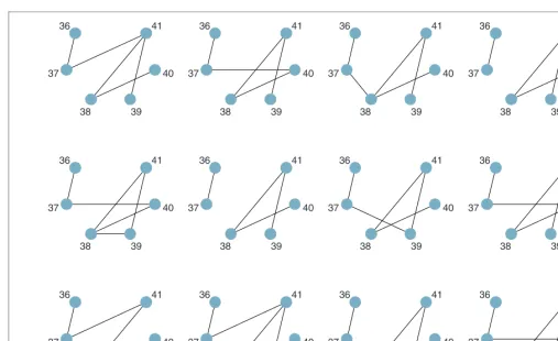
Forward stepwise analysis of SNP36–SNP41
This group of markers was selected because they mark the join between two apparent regions of high LD (Figure 1). The models derived from this more complex region are shown in Figure 3. In this more complex example, model repeatability was lower. The strong block-like relationship among markers SNP38–SNP41 was clearly visible as a tangle of graphical relationships in each bootstrap sample, but the exact positioning of edges tended to vary. Lowering the threshold for parameter inclusion fromp¼0.05 top¼0.01 led to the loss of edges in every bootstrap sample (Figure 4). At this lower threshold, the two regions of high LD (SNP36–SNP37 and SNP38–SNP41) became more visibly distinct. Few model changes were observed as the threshold was lowered fromp¼0.01 top¼0.001 (results not shown).
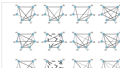
Forward stepwise analysis of SNP44–SNP49
Lastly, for SNP44–SNP49, the LD plot (Figure 1) suggests a complex set of interrelationships. The parsimonious modelsfor the 12 bootstrap samples are given in Figure 5. The large number of edges suggests that this is an area of high haplotype diversity and this interval provides the most striking example of lack of repeatability in model fitting. Only two features were captured in all models. These were a three-way interaction (SNP46, SNP47, SNP48) and a two-way interaction (SNP44, SNP45). Other features were variously described. This is a clear example where overall variability of relationship can be explained in a model in a number of ways.
Discussion
This study investigated the performance of stepwise log-linear modelling in the evaluation of LD in three genomic loci. Bootstrapping of the data demonstrated that although certain LD features were consistently captured by this approach, derived models were generally not repeatable. Furthermore, altering the significance threshold for inclusion of parameters in the stepwise analysis did not materially change our models. It is noteworthy that sample size may be a consideration. Repeating the bootstrap analyses with a smaller sample size (n¼75) led to models with a greater number of higher-order interactions (results not shown). With a sample size of n¼150, these same relationships tended to manifest as 41
40
39 38
37
36 41
40
39 38
37
36 41
40
39 38
37
36 41
40
39 38
37 36
41
40
39 38
37
36 41
40
39 38
37
36 41
40
39 38
37
36 41
40
39 38
37 36
41
40
39 38
37
36 41
40
39 38
37
36 41
40
39 38
37
36 41
40
39 38
37 36
Figure 4.Graphical images of the models derived by a log-linear modelling of data from single nucleotide polymorphism (SNP)36–SNP41. Ap-value threshold of 0.01 was used. The 12 graphs depict models derived from 12 bootstrap samples. A node represents a SNP and an edge denotes a pairwise interaction.
Mander and Bansal
two-way interactions in the model. Clearly, the allele frequency distribution of the markers available must be a major component of the patterns derived, and while it is not appropriate to extrapolate our findings to all genomic regions and/or all methodologies, these findings do raise interesting questions of repeatability. LD-based inference is widely used, both for exploratory analysis and for the efficient selection of markers for genotyping.
Model complexity and/or lack of repeatability should come as no real surprise. LD mapping exploits historical recombination events to narrow candidate regions for disease genes; however, the pattern of LD is also influenced by mutation and other stochastic factors which create associations between markers that do not have a simple relationship with distance. Our models shed no light on the ‘source’ of any complexity; they merely support its existence. Greater repeatability of inferred LD has been observed at compara-tively low resolution, when a close relationship is maintained between recombination and LD patterns.6Our models reflect the more stochastic picture seen at comparatively high resolution.
Other investigators have presented methods of modelling non-adjacent SNP interactions. Thomas and Camp12derived Bayesian graphical models using a tailored
Metropolis–Hastings approach. Earlier evaluations of partial LD models have also been made. One group commented on the exceeding complication arising from the inclusion of higher-order interactions.24Model complexity is indeed an outcome of applying this method to a large genomic region. In terms of applicability, our approach is limited to a relatively small number of SNPs — fewer than ten — and thus it is restricted to small genomic regions. For most current-day situations, it would be impractical to apply stepwise log-linear modelling for the purposes of tag selection. The great wealth of marker data available now from the HapMap and other sources, combined with the ever-decreasing cost of genotyp-ing, make it an unlikely avenue to pursue. For small candidate gene studies, however, it would be possible to use a log-linear approach to identify ‘sensible’ models to test in the analysis of a subsequent replication study, thereby reducing the burden of multiple testing. Such models would include an
additional parameter pertaining to the disease locus but would be derived in exactly the same way. It is hoped that the visual immediacy of this approach will aid hypothesis gener-ation and serve as a useful addition to a fine-mapping tool kit that already includes coalescent modelling,25for example.
It is now generally agreed that the genome is not simply composed of discrete haplotype blocks of uniformly high LD;
49
48
47 46
45
44 49
48
47 46
45
44 49
48
47 46
45
44 49
48
47 46
45 44
49
48
47 46
45
44 49
48
47 46
45
44 49
48
47 46
45
44 49
48
47 46
45 44
49
48
47 46
45
44 49
48
47 46
45
44 49
48
47 46
45
44 49
48
47 46
45 44
indeed, our models support a more complex reality. Nevertheless, LD has an important role to play in designing efficient marker sets for genetic study. Resources such as the HapMap lessen the need for marker validation and provide a means of allowing the selection of informative markers for genotyping. Our bootstrap results show that LD-based inference can be sample dependent, even within an ethnic group. Therefore, in utilising such data, it may be beneficial to investigate the repeatability of one’s chosen methodology and, if appropriate, to allow greater redundancy in marker selection.
Acknowledgments
The authors would like to thank members of the Statistics and Programming Department, and members of the Discovery and Pipeline Genetics Department at GlaxoSmithKline, for helpful discussions and input, particularly Karen Lewis and Chun-Fang Xu, for sharing the data described here.
References
1. Clark, A.G. (1990), ‘Inference of haplotypes from PCR-amplified samples
of diploid populations’,Mol. Biol. Evol.Vol. 7, pp. 111–122.
2. Excoffier, L. and Slatkin, M. (1995), ‘Maximum-likelihood estimation
of molecular haplotype frequencies in a diploid population’,Mol. Biol.
Evol.Vol. 12, pp. 921–927.
3. Stephens, M., Smith, N.J. and Donnelly, P. (2001), ‘A new statistical
method for haplotype reconstruction from population data’,Am. J. Hum.
Genet.Vol. 68, pp. 978–989.
4. Niu, T., Qin, Z.S., Xu, X.et al.(2002), ‘Bayesian haplotype inference for
multiple linked single-nucleotide polymorphisms’,Am. J. Hum. Genet.
Vol. 70, pp. 157–169.
5. Daly, M.J., Rioux, J.D., Schaffner, S.F.et al.(2001), ‘High-resolution
haplotype structure in the human genome’,Nat. Genet.Vol. 29,
pp. 229–232.
6. Jeffreys, A.J., Kauppi, L. and Neumann, R. (2001), ‘Intensely punctuate meiotic recombination in the class II region of the major
histocompatibility complex’,Nat. Genet.Vol. 29, pp. 217–222.
7. Patil, N., Berno, A.J., Hinds, D.A.et al.(2001), ‘Blocks of limited
haplotype diversity revealed by high resolution scanning of human
chromosome 21’,ScienceVol. 294, pp. 1719–1723.
8. Gabriel, S.B., Schaffner, S.F., Nguyen, H.et al.(2002), ‘The structure of
haplotype blocks in the human genome’,ScienceVol. 296, pp. 2225–2229.
9. Twells, R.C.J., Mein, C.A., Phillips, M.S.et al.(2003), ‘Haplotype
structure, LD blocks, and uneven recombination within the LRP5 gene’,
Genome Res. Vol. 13, pp. 845–855.
10. Schwartz, R., Halldorsson, B.V., Bafna, V.et al.(2003), ‘Robustness of
inference of haploype block structure’,J. Comp. Biol. Vol. 10, pp. 13–19.
11. Johnson, G.C.L., Esposito, L., Barratt, B.J.et al.(2001), ‘Haplotype
tagging for the identification of common disease genes’,Nat. Genet.
Vol. 29, pp. 233–237.
12. Thomas, A. and Camp, N.J. (2004), ‘Graphical modeling of the joint
distribution of alleles at associated loci’,Am. J. Hum. Genet.Vol. 74,
pp. 1088–1101.
13. Morris, A., Pedder, A. and Ayres, K. (2003), ‘Linkage disequilibrium
assessment via log-linear modeling of SNP haplotype frequencies’,Genet.
Epidemiol.Vol. 25, pp. 106–114.
14. Huttley, G.A. and Wilson, S.R. (2000), ‘Testing for concordant equilibria
between population samples’,GeneticsVol. 156, pp. 2127–2135.
15. Goldstein, D.B. (2001), ‘Islands of linkage disequilibrium’,Nat. Genet.
Vol. 29, pp. 109–111.
16. Holmes, D., Fitzgerald, P., Goldberg, S.et al.(2000), ‘The PRESTO
(Prevention of restenosis with tranilast and its outcomes) protocol: A
double-blind, placebo-controlled trial’,Am. Heart J.Vol. 139, pp. 23–31.
17. Danoff, T.M., Campbell, D.A., McCarthy, L.C.et al.(2004), ‘A Gilbert’s
syndrome UGT1A1 variant confers susceptibility to tranilast-induced
hyperbilirubinemia’,Pharmacogenomics J. Vol. 4, pp. 49–53.
18. Xu, C.F., Lewis, K.F., Yeo, A.J.et al.(2004), ‘Identification of
pharmacogenetic effect by linkage disequilibrium mapping’,
Pharmacogenomics J.Vol. 4, pp. 374–378.
19. Chiano, M.N. and Clayton, D.G. (1998), ‘Fine genetic mapping using
haplotype analysis and the missing data problem’,Ann. Hum. Genet.
Vol. 62, pp. 55–60.
20. Mander, A.P. (2001), ‘Haplotype analysis in population-based association
studies’,Stata JournalVol. 1, pp. 58–75.
21. Wilkinson, G. and Rogers, C. (1973), ‘Symbolic description of factorial
models for analysis of variance’,Appl. Stat.Vol. 22, pp. 392–399.
22. StataCorp (2001),Stata Statistical Software: Release 7.0, StataCorp LP,
College Station, TX.
23. Wall, J.D. and Pritchard, J.K. (2003), ‘Assessing the performance of the
haplotype block model of linkage disequilibrium’,Am. J. Hum. Genet.
Vol. 73, pp. 502–515.
24. McPeek, M.S. and Strahs, A. (1999), ‘Assessment of linkage disequilibrium by the decay of haplotype sharing, with application to fine-scale genetic
mapping’,Am. J. Hum. Genet.Vol. 65, pp. 858–875.
25. Morris, A.P., Whittaker, J.C. and Balding, D.J. (2002), ‘Fine-scale mapping of disease loci via shattered coalescent modelling of genealogies’,
Am. J. Hum. Genet.Vol. 70, pp. 686–707.
Mander and Bansal


![Zinc sulfate as an adjunct to methylphenidate for the treatment of attention deficit hyperactivity disorder in children: A double blind and randomized trial [ISRCTN64132371]](data:image/gif;base64,R0lGODlhAQABAIAAAP///wAAACH5BAEAAAAALAAAAAABAAEAAAICRAEAOw==)