www.the-cryosphere.net/6/21/2012/ doi:10.5194/tc-6-21-2012
© Author(s) 2012. CC Attribution 3.0 License.
The Cryosphere
Reformulating the full-Stokes ice sheet model for a more efficient
computational solution
J. K. Dukowicz
Climate, Ocean, and Sea-Ice Modeling (COSIM) Project, Group T-3, MS B216, Los Alamos National Laboratory, Los Alamos, New Mexico, 87545, USA
Correspondence to: J. K. Dukowicz ([email protected])
Received: 25 May 2011 – Published in The Cryosphere Discuss.: 1 July 2011
Revised: 21 November 2011 – Accepted: 12 December 2011 – Published: 6 January 2012
Abstract. The first-order or Blatter-Pattyn ice sheet model, in spite of its approximate nature, is an attractive alterna-tive to the full Stokes model in many applications because of its reduced computational demands. In contrast, the unap-proximated Stokes ice sheet model is more difficult to solve and computationally more expensive. This is primarily due to the fact that the Stokes model is indefinite and involves all three velocity components, as well as the pressure, while the Blatter-Pattyn discrete model is positive-definite and in-volves just the horizontal velocity components. The Stokes model is indefinite because it arises from a constrained min-imization principle where the pressure acts as a Lagrange multiplier to enforce incompressibility. To alleviate these problems we reformulate the full Stokes problem into an un-constrained, positive-definite minimization problem, similar to the Blatter-Pattyn model but without any of the approxi-mations. This is accomplished by introducing a divergence-free velocity field that satisfies appropriate boundary condi-tions as a trial function in the variational formulation, thus dispensing with the need for a pressure. Such a velocity field is obtained by vertically integrating the continuity equation to give the vertical velocity as a function of the horizontal velocity components, as is in fact done in the Blatter-Pattyn model. This leads to a reduced system for just the horizon-tal velocity components, again just as in the Blatter-Pattyn model, but now without approximation. In the process we obtain a new, reformulated Stokes action principle as well as a novel set of Euler-Lagrange partial differential equations and boundary conditions. The model is also generalized from the common case of an ice sheet in contact with and sliding along the bed to other situations, such as to a floating ice shelf. These results are illustrated and validated using a sim-ple but nontrivial Stokes flow problem involving a sliding ice sheet.
1 Introduction
The most general and accurate model currently used for the simulation of ice sheet dynamics is based on non-Newtonian Stokes flow (e.g., Greve and Blatter, 2009). At present, how-ever, a full-Stokes model presents formidable challenges for large-scale modeling, although such models exist and are being used (e.g., Zwinger and Moore, 2009, implemented in the ELMER (http://www.csc.fi/english/pages/elmer) code package). As a consequence, there is considerable interest in various approximate models (e.g., the first order or Blatter-Pattyn approximation, and the shallow ice and shallow shelf approximations) that are more limited but computationally far cheaper (e.g., Pattyn et al., 2008).
Typically, a discretized Stokes model may be written in matrix form as
A G GT 0
ui P
=
bi
q
, (1)
whereA=AT is a square, symmetric, positive-definite ma-trix representing the negative of the discrete nonlinear stress divergence operator in the momentum equations,ui is a
the pressure. Second, large-scale saddle point problems are typically solved iteratively using Krylov subspace methods (conjugate gradient-type algorithms). Such methods tend to converge slowly and are prone to failure when applied to sad-dle point problems, so it is necessary to find and apply a good preconditioner to achieve reasonable convergence. In fact, there is a voluminous literature on appropriate methods for the numerical solution of saddle point problems (see Benzi et al. (2005), for example). Finally, in the finite element context, basis functions for the pressure and velocity have to be chosen carefully so that the discrete problem is well posed (this involves satisfying the so-called Brezzi-Babuska or inf-sup condition, see Brezzi and Fortin (1991) or Elman et al. (2005), for example).
In glaciology, these difficulties have typically been avoided by the use of an approximate Stokes model, the so-called first-order model, otherwise so-called the Blatter-Pattyn model, first introduced by Blatter (1995) and refined by Pat-tyn (2003). The Blatter-PatPat-tyn model is obtained by invok-ing the small aspect ratio approximation, i.e., assuminvok-ing that the ratio of the characteristic vertical and horizontal length scales in the ice sheet velocity field is small, thus neglecting the mixed horizontal-vertical stress tensor components. As a result, it becomes possible to vertically integrate the verti-cal momentum equation and the continuity equation to obtain pressure as a function of the vertical velocity,P=P (w), and the vertical velocity as a function of the horizontal velocity components,w=w(u(i))(see Pattyn, 2003). This allows the
elimination of both the pressure and vertical velocity from the approximated Stokes model to obtain a reduced system in terms of the horizontal velocity components only, which may be expressed in matrix form as follows
˜
Au(i)= ˜b(i), (2)
where the index (i) represents just the horizontal compo-nents, andA˜ is a symmetric, positive-definite matrix of re-duced rank (of order 2N )as compared to the system matrix in Eq. (1). In contrast to Eq. (1), the system corresponding to Eq. (2) is associated with the minimization of a positive-definite functional and is therefore ideally suited to solu-tion by Krylov subspace methods (Knoll and Keyes, 2004) or even by direct numerical optimization methods (Nocedal and Wright, 2006). As a result, the Blatter-Pattyn system is much easier to solve than the full Stokes system. However, the Blatter-Pattyn model is much more limited in application (e.g., see the discussion and results in Pattyn et al., 2008). This is because of the small aspect ratio approximation and, in addition, because of a further approximation implicitly built into the Blatter-Pattyn model, limiting it to small basal slopes (see Dukowicz et al., 2011, henceforth referred to as DPL11). To partially remedy this last problem, DPL11 intro-duced a second Lagrange multiplier,3, to enforce tangential flow at the base.
In the present paper we make the observation that there is no need for Lagrange multipliersP and3if one already
has a velocity field that satisfies both continuity and the basal no-penetration boundary condition for use as a trial function in a variational formulation, in loose analogy with the Ritz method. We note that such a velocity field is available, at least in principle, from vertically integrating the continuity equation to obtain the vertical velocity in terms of horizon-tal velocities,w u(i), as is done in the Blatter-Pattyn model.
In Dukowicz et al. (2010) (henceforth referred to as DPL10) and in DPL11 it was shown that non-Newtonian Stokes flow, including boundary conditions, may be expressed as a con-strained variational principle expressed in terms of an ac-tion funcac-tional,AS[ui,P ,3], whose arguments represent the
functions with respect to which a stationary point is to be found. Eliminating the vertical velocity from the Stokes ac-tion, we obtain the “reformulated” Stokes acac-tion, as follows ARSu(i)=ASu(i),w u(i),P=0,3=0, (3)
which, together withw=w u(i)forms a complete
specifi-cation of the Stokes problem. Note the following properties: (a) the actionARSu(i)is exactly equivalent to the Stokes
action, as indicated in Eq. (3), (b) since both Lagrange mul-tipliers are zero, the reformulated action is positive-definite, just as in the Blatter-Pattyn model, and (c) this action leads to a matrix system of exactly the same form as Eq. (2). The resulting matrix system, therefore, has exactly the same ben-eficial properties as the Blatter-Pattyn system, except now without approximation.
It is interesting to note that Pattyn (2008) presents a refor-mulation of the full Stokes model that superficially resem-bles the Blatter-Pattyn model. However, this reformulation basically amounts to expressing the pressureP in terms of an alternative variable, the vertical stress componentτzz, and
thus leads to an iteration scheme that is effectively equiva-lent to the solution of a system in the form of Eq. (1). One feature of the present reformulation is that it, in effect, leads to an integro-differential formulation of the Stokes problem. Integro-differential formulations have appeared previously in the glaciological literature (e.g., Van der Veen and Whillans, 1989; Hindmarsh, 1993). These early formulations appear to involve the vertical integral of the shear stress τxz and
are therefore different in substance and motivation from the present formulation.
implementation of the present method, and thereby provide some justification for the claims of computational efficiency, by means of a relatively simple but nontrivial test problem involving the sliding of an ice sheet along an inclined plane. This test problem is particularly attractive because it also pro-vides an analytical solution, which helps in the understanding of the present method and makes it easy to check the validity and accuracy of the numerical solution. For completeness, in Sect. 6 we also obtain the corresponding reformulated Euler-Lagrange partial differential equations and boundary condi-tions. These equations may be of interest for comparison with the full Stokes system of equations, and possibly may also suggest other approximations, perhaps more accurate, to the Stokes model. Finally, in Sect. 7 we summarize and draw some conclusions.
2 The basic Stokes model
We begin with the variational principle for the non-Newtonian ice sheet Stokes model whose action functional (see DPL11) is given by
AS[ui,P ,3s,3b]=
R
VdV
Gn ε˙2
−ρgiui−P∂u∂xii
+R
S(s)dS 3s(P−Ps)+RS(b)dS 3buini−6j(u)nj,
(4) whereui ∈ {u,v,w}is the three dimensional velocity
vec-tor,gi is the gravitational acceleration vector (typicallygi= (0,0,−g)),ρ is the ice density, assumed constant, andε˙2= ˙
εijε˙ijis the second invariant of the full Stokes strain-rate
ten-sor, where
˙
εij=
1 2
∂u
i ∂xj
+∂uj
∂xi
,
such that, expanded in Cartesian coordinates, we have
˙
ε2=
∂u
∂x 2
+
∂v
∂y 2
+
∂w
∂z 2
+1
2 (5)
" ∂u
∂y+ ∂v ∂x
2
+
∂u
∂z+ ∂w
∂x 2
+
∂v
∂z+ ∂w
∂y 2#
.
We define Gn
˙
ε2= 2n
n+1µn
˙
ε2ε˙2, (6)
where µn
˙
ε2
=µ0(θ )
˙
ε2
(1−n)/2n
, (7)
is the Glen’s law viscosity coefficient, typically used with exponentn=3, andµ0(θ )is a temperature-dependent
co-efficient. As in DPL10 and DPL11, we illustrate the effect of basal stress forces by6j(u)= −βuiuinj2, which
rep-resents a linear frictional sliding law with a constant coeffi-cient,β; β≥0. However, other frictional laws are easily ac-commodated as in Schoof (2010), for example. The three in-tegrals above cover the entire ice sheet volume and its upper
and basal surfaces, respectively. Here,xi∈ {x,y,z}is the
po-sition vector, andniis the outward-pointing unit vector at the
ice sheet bounding surfaces. Note that Cartesian tensor no-tation is being used, and, where appropriate, the summation convention on repeated indices. In general, tensor indices are three-dimensional, i.e.,i,j,··· ∈ {x,y,z}, except when an index appears in parentheses, in which case it denotes an index in the horizontal plane only, e.g., (i),(j ),··· ∈ {x,y}, so that, for example,u(i)∈ {u,v}, uiui=u2+v2+w2 and u(i)u(i)=u2+v2.
As mentioned previously, the functional, Eq. (4), repre-sents a constrained minimization principle, with constraints enforced by three Lagrange multipliers,P,3s, and3b. The
pressureP enforces incompressibility, and3benforces
tan-gential flow at the base. In spite of its role as a Lagrange multiplier, pressure also has a physical role in the presence of gravity. For instance, in the case of static flow (maintained by confining walls, for example), the pressure satisfies a hydro-static balance equation and therefore we need an upper sur-face boundary condition,P=Ps, wherePs is some known
or somehow specified pressure at the upper surface. Very fre-quently, we havePs=0 if there is no ice or water weighing
down from above. In the general case, the pressure will also require a separate boundary condition at the upper surface, andP =0 is appropriate if atmospheric pressure is negligi-ble. This condition is enforced by3s. Alternatively, in many
cases it may be simpler to directly insert such a boundary condition into the matrix equation.
The variational principle states that the solution of this dynamical system in terms of the arguments, i.e., the ve-locity componentsui, pressureP, and Lagrange multipliers 3s,3b, is to be found at the stationary point of the action,
obtained by setting the functional derivatives with respect to the arguments equal to zero, as follows
δAS δui
=0, δAS
δP =0, δAS δ3s
=0, δAS
δ3b
=0. (8)
This yields the following Euler-Lagrange equations: (a) A three-dimensional momentum equation, ∂σij
∂xj
+ρgi= ∂τij ∂xj
−∂P
∂xi
+ρgi=0, (9)
whereσij=τij−P δij is the Cauchy stress tensor andτij=
2µn(ε˙2)ε˙ij is the deviatoric stress tensor, and (b) the
continu-ity equation for incompressible flow, ∂ui
∂xi
=0. (10)
In addition, the following boundary conditions are implied. At the upper surfaceS(s), specified at any instant of time by z=zs(x,y,t ), we have (c) stress-free boundary conditions
P=Ps, (11)
n(s)
Ice Sheet
n(b)
Bed
Upper Surface
Basal Surface
x z
Fig. 1. A schematic diagram of the simplified ice sheet configura-tion considered in this paper.
and, using (10), we have deduced thatAs=0. Along a fixed
basal surfaceS(b), specified byz=zb(x,y), we have (d)
fric-tional tangential sliding boundary conditions
u(b)i n(b)i =0, (13)
τijn(b)j −
n(b)k τkjn(b)j
n(b)i +βu(b)i =0. (14)
The variational principle actually yields an equation contain-ing3b−P, but this is easily eliminated, as in DPL11, to
obtain Eq. (14). The unit normal vectors that appear here are defined as follows
n(s)j =n(s)x , n(s)y , n(s)z T= (−∂zs/∂x,−∂zs/∂y,1) T
q
1+(∂zs/∂x)2+(∂zs/∂y)2 ,(15)
n(b)j =
n(b)x , n(b)y , n(b)z T= ∂zb
∂x,∂zb
∂y,−1T
q
1+ ∂zb
∂x2+ ∂zb
∂y2 . (16)
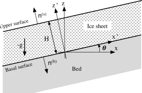
For clarity, we employ superscripts (s) and (b), and sub-scriptssandb, to indicate an upper surface or basal value, respectively, particularly in those cases where confusion is possible. For concreteness, we have assumed a simplified ice sheet configuration illustrated in Fig. 1 that is subject to boundary conditions Eqs. (11–14), namely, an upper surface entirely exposed to the atmosphere and a basal surface that is entirely in contact with and sliding along a rigid bed. Fur-ther, for the purpose of this paper we implicitly define the upper surface by the conditionn(s)z >0, and the basal
sur-face byn(b)z <0. We have chosen to use this commonly used
configuration since there are great many possibilities and it is impossible to deal with them all. The Stokes model itself is of course entirely general. In the next Section we shall in-dicate how to generalize to a moving and possibly melting basal surface, as at the base of a floating ice shelf.
3 Generalizing the basal boundary condition
So far we have assumed a fixed and rigid basal surface spec-ified byz=zb(x,y). In such a case the no-penetration
con-dition, Eq. (13), is given by w(b)=u(b)(i) ∂zb
∂x(i)
. (17)
More generally, for a moving material surface (i.e., a La-grangian surface with no inflowing or outflowing flux due to a gain or loss of mass crossing the surface) and specified by z=zb(x,y,t ), we have
w(b)=∂zb
∂t +u (b) (i)
∂zb ∂x(i)
. (18)
In addition, assuming an outwardly directed flux of mass at the basal surface with a normal velocity of magnitudeun,
which may be due to melting, ablation, etc., we obtain w(b)=wn(b)+u(b)(i) ∂zb
∂x(i)
, (19)
where w(b)n =∂zb∂t−un
q
1+ ∂zb∂x2+ ∂zb∂y2 is
the effective basal vertical velocity due to both the motion of the interface and an outflowing mass flux. In general, and in particular at the base of a floating ice shelf, we might ex-pect thatwn(b)6=0. For our present purpose we assume that it
is a given quantity. In general, however, the velocityw(b)n is
unknown and must be determined by the simultaneous solu-tion of the ice sheet problem and the external environment.
Integrating the continuity equation, Eq. (10), in the vertical direction with Eq. (19) as the boundary condition, the vertical velocity is given by
w=w(b)n +u(b)(i) ∂zb ∂x(i)
−
Z z
zb
∂u(i) ∂x(i)
dz0, (20)
or, alternatively, using Leibniz’s theorem, one obtains w=w(b)n − ∂
∂x(i)
Z z
zb
u(i)dz0. (21)
Either one of these expressions corresponds to the relation w=w u(i) referred to earlier. The choice between them
will depend on which is preferable from the point of view of discretization.
We note thatw(b)n will vanish along certain sections of the
ice sheet basal surface (i.e., when the ice sheet is sliding in contact with a fixed and rigid bed) but may have nonzero val-ues elsewhere. It is therefore to be considered as a general function of the horizontal position vectorx(i)over the entire
without loss of generality. However, in general we might ex-pect thatβ is zero whenw(b)n is nonzero and vice versa, so
thatβw(b)n =0. In the following, we shall assume this to be
true, while leaving open the possibility of exceptions under unusual circumstances.
4 The reformulated action principle
As discussed in Sect. 1, the Lagrangian multipliersP and 3b are no longer needed if the vertical velocity given by
Eqs. (20) or (21) is used in the action functional. This is be-cause the three-dimensional velocity field, given by the hor-izontal velocity components and the vertical velocity from Eqs. (20) or (21), already satisfies the continuity equation, Eq. (10), and the correct basal boundary condition, Eq. (13). Furthermore, eliminatingP also removes the need for3s.
Substituting this velocity field into Eqs. (4) and (5), the vari-ational principle now becomes a function of horizontal ve-locity only,
ARS
u(i)
=
Z
V dVhGn
˙
ε2RS+ρgw u(i)
i
(22)
−
Z
S(b)
dS 6j000u(b)n(b)j ,
where
˙
ε2RS= ∂u ∂x
2
+
∂v ∂y
2
+
∂u ∂x+
∂v ∂y
2
+1
2
∂u ∂y+
∂v ∂x
2
+1 2
∂u ∂z+
∂w(u(i))
∂x
2
+∂v
∂z+ ∂w(u(i))
∂y
2 ,
(23)
6000j
u(b)
n(b)j = −1
2β "
u(b)(i)u(b)(i)+
w(b)n +u(b)(i) ∂zb ∂x(i)
2# , (24)
andw u(i)
is given by either Eq. (20) or (21). The subscript RS stands for “Reformulated Stokes”. Observe thatε˙RS2 is actually the same asε˙2since the velocity fields in the Stokes and reformulated Stokes cases are the same. In general, the term involvingw(b)n vanishes in Eq. (24) because of our
as-sumption thatβw(b)n =0.
The action, Eq. (22), may be simplified somewhat. As shown in Appendix A, the gravitational work term in Eq. (22) is expressible as follows
Z
V
dV w u(i)
=
Z
V dV u(i)
∂zs ∂x(i)
+
Z
V
dV wn(b). (25) The last term on the right hand side is independent ofu(i); as
such, it does not participate in the variational principle and may be omitted. Substituting this into Eq. (22), the action takes the following alternative form,
A0RSu(i)=
Z
V dV
Gn
˙
ε2RS+ρgu(i) ∂zs ∂x(i)
(26)
−
Z
S(b)
dS 6000j
u(b)n(b)j .
n(s)
n(b)
Bed
Upper surface
Basal surface
x
z
-g
H
x
'
z
'
Ice sheet
Fig. 2. The simple sliding ice sheet test problem configuration, showing the transformed (rotated) coordinate system, x0, z0.
It may be observed that both functionals (excluding gravi-tational terms since they are only responsible for the forcing) are positive-definite, in contrast to the standard Stokes func-tional. Therefore, the variational principle is now a true min-imization problem subject to gravitational forcing, just as in the Blatter-Pattyn approximate model. Also, as noted before, this is a fully three-dimensional problem in only two vari-ables, i.e., the two horizontal velocity components, again as in the Blatter-Pattyn model. Furthermore, all boundary con-ditions are automatically and correctly incorporated, includ-ing the basal no-penetration (or tangential flow) boundary condition. Note that these functionals are to be used jointly with Eq. (20) or (21), as emphasized in Eqs. (22–24), to ob-tain the complete three-dimensional velocity field.
This action, Eq. (26), (or alternatively, Eq. (22)) is the pre-ferred starting point for a numerical solution of the problem. This is because the discretization of the variational princi-ple applied to the action automatically yields a symmetric, positive-definite matrix problem, analogous to Eq. (2), which is optimal for an efficient numerical solution, as discussed earlier. However, one possible disadvantage of this reformu-lation is that the action contains higher order derivatives than in the standard case, which may impose additional continu-ity requirements on the approximating space. A discussion of the requirements for the approximation space, however, is beyond the scope of the present paper.
5 A simple test problem
The problem is very attractive because it provides a non-trivial analytic Stokes flow solution that is relevant to ice sheets. Moreover, the problem can be reduced from a two dimensional configuration to a one-dimensional problem by rotating the coordinate system counterclockwise by an an-gleθ, i.e.,(x, z)→ x0,z0, to align it with the ice slab. In this case all variables will be functions solely ofz0since the problem is longitudinally isotropic and extends to infinity in lateral directions. In addition, we have velocityv=0 since there is no forcing in the transverse direction. In spite of its simplicity and linearity, this problem is nevertheless still use-ful as a means of evaluating the computational properties of the reformulated model in comparison to the standard formu-lation.
The required coordinate transformation is given by x0= xcosθ+zsinθ, x=x0cosθ−z0sinθ,
z0= −xsinθ+zcosθ, z=x0sinθ+z0cosθ, (27) and therefore ice velocities transform as follows
u0= ucosθ+wsinθ, u=u0cosθ−w0sinθ,
w0= −usinθ+wcosθ, w=u0sinθ+w0cosθ. (28) Since∂∂x0=0, we obtain
∂ ∂x=
∂z0 ∂x
d
dz0= −sinθ d dz0,
∂ ∂z=
∂z0 ∂z
d
dz0=cosθ d dz0.(29) Note that the basal surface is located atz0=0, the upper sur-face atz0=H, and the unit normal vectors are given by
n(s)x = −sinθ, n(s)z = cosθ, n(b)x = sinθ, n(b)z = −cosθ.
(30)
5.1 The analytic Stokes flow solution
Let us nondimensionalize by introducing a velocity scale ρgH2µ, a length scaleH, and a pressure scaleρgH. As a result, the problem is characterized by only two independent nondimensional parameters, the angle of inclinationθ, and a basal friction parameterη=βHµ. In this section, there-fore, we shall consider all variables to be nondimensional. In transformed coordinates, the nondimensional Stokes system of momentum equations, Eq. (9), becomes
d2u dz02+sinθ
dP dz0 =0,
d2w dz02−cosθ
dP
dz0−1=0, (31) while the continuity equation, Eq. (10), is given by
−sinθdu dz0+cosθ
dw
dz0 =0. (32)
These equations may be combined to obtain a separate equa-tion for each of the three variables, as follows
d2u
dz02−sinθcosθ=0,
d2w dz02−sin
2θ=0, (33)
dP
dz0+cosθ=0. (34)
Note that Eq. (34) represents hydrostatic balance; this again reinforces the conclusion that pressure requires a separate boundary condition at the surface.
Boundary conditions at the stress-free surface z0=1 , Eqs. (11) and (12), are given by
P=0,
1+sin2θdzdu0−sinθcosθdwdz0+sinθ P=0,
−sinθcosθdzdu0+ 1+cos2θ dw
dz0−cosθ P=0,
(35)
where for simplicity we have assumed thatPs=0. Actually,
in this simple test problem the pressure boundary condition is superfluous since, making use of the continuity equation, Eq. (32), the last two equations of Eq. (35) already implyP=
0. Thus, simplifying Eq. (35), the upper surface boundary conditions become
P=0, du dz0=0,
dw
dz0=0. (36)
Similarly, the basal surface z0=0
boundary conditions, Eqs. (13), (14), become
sinθ u−cosθ w=0,
−cosθ
cosθdzdu0+sinθdwdz0
+ηu=0,
−sinθ
cosθdzdu0+sinθdwdz0
+ηw=0.
(37)
These are not independent. Simplifying, we therefore obtain the remaining two basal boundary conditions, as follows
du
dz0−ηu=0, dw
dz0−ηw=0. (38)
Finally, the system consisting of Eqs. (33), (34), (36), and (38) may be solved to obtain
u=sinθcosθ 1
2z
02−z0−1 η
, (39)
w=sin2θ 1
2z
02−z0−1 η
, P=cosθ 1−z0.
This solution represents ice flowing parallel to the base with an upper surface velocity of magnitude(η+2)sinθ2ηand a basal velocity of magnitude sinθη. Since the velocity mag-nitude is proportional to sinθ, the ice ceases to flow when the slab is horizontal, and conversely, velocity reaches its maximum value when the slab is oriented vertically. In the absence of friction(η→0)there is nothing to oppose grav-ity and velocgrav-ity becomes infinite, while for an infinite fric-tion parameter(η→ ∞)surface velocity goes to sinθ
5.2 Variational formulations for the Stokes and the reformulated Stokes test problems
In the present case, the Stokes action, Eq. (4), per unit cross-sectional area, may be written as follows
AS[u,w,P ,3s,3b]=
1 2
Z z0=1
z0=0 dz0 "
du dz0
2
+
dw dz0
2
+
sinθdu
dz0−cosθ dw dz0
2#
+
Z z0=1
z0=0 dz0P
sinθdu
dz0−cosθ dw dz0
+3sp(1)+3b(sinθ u(0)−cosθ w(0))
+1
2η
u(0)2+w(0)2+
Z z0=1
z0=0 dz0w.
(40)
This incorporates all boundary conditions. As noted above, since the surface pressure boundary condition is superflu-ous we might simply set 3s=0, although this is not
nec-essary. The corresponding action principle leads to a one-dimensional Euler-Lagrange system of equations and ary conditions, i.e., an ordinary differential equation bound-ary value problem for the three variables, u,w,P, and the basal boundary constant, 3b, that is entirely equivalent to
the system of Eqs. (31), (32), (35), (37).
In a similar manner, the reformulated Stokes action, Eq. (22), becomes
ARS[u]=
Z z0=
1
z0=0 dz0
" 2sin2θ
du dz0
2 +1
2
cosθdu dz0−sinθ
dw(u) dz0
2#
(41)
+1
2sec
2θ η u2 z0=0+
Z z0=1
z0=0
dz0w(u) ,
where
w(u)=tanθ d dz0
Z z0
0
udz00 (42)
corresponds to Eq. (21), although Eq. (20) could have been used. Note that in the present case we havewn(b)=0. Eq. (42)
is retained in this form as a reminder that this is what is dis-cretized in the general, multidimensional case. However, in the present case it is more convenient write it in its equivalent form,
w(u)=tanθ u. (43)
Substituting this in Eq. (41), we obtain
ARS[u]=
Z z0=1
z0=0 dz0
" 1 2sec
2θ
du
dz0 2
+tanθ u #
(44)
+1
2sec
2θ η u2 z0=0.
The variation of action, Eq. (44), results in a single Euler-Lagrange equation,
d2u
dz02−sinθcosθ=0, (45)
and boundary conditions, du
dz0
z0=1
=0, du
dz0−η u
z0=0
=0. (46)
This agrees with the horizontal part of the Stokes system from Eqs. (33), (36), and (38), and therefore leads to exactly the same solution as given in Eq. (39).
5.3 Discretization of the standard Stokes action Let us now introduce a uniform one-dimensional grid with cell widthh=1N, whereN is the number of cells. The cells are indexed byk∈ {1,2,···,N}, and cell nodes by k∈ {0,1,2,···,N}, such thatz0k=k h. Thus, cellkis bounded by nodekon the right and nodek−1 on the left. We assume that discrete velocity values are located at nodes, resulting in a piecewise linear velocity distribution, as follows
u z0=1
h N
X
k=1
huk−1+(uk−uk−1) z0−z0k−1
; (47)
z0k−1≤z0≤zk0,
and similarly for the vertical velocity componentw. Noting that pressure is specified at the upper surface, it is convenient to also assume a piecewise linear distribution for the pres-sure, analogous to Eq. (47), as follows
P z0=1
h N
X
k=1
hPk−1+(Pk−Pk−1) z0−z0k−1
; (48)
z0k−1≤z0≤zk0,
and specifically setPN=0, or else enforce this condition by
using the Lagrange multiplier3s. We have already noted
that in general there are subtle issues in connection with the choice of basis functions for pressure and velocity in saddle point problems, and in the Stokes system in particular. In the present case, if we use the pressure distribution, Eq. (48), and do not setPN=0, we obtain a singular problem. On the
other hand, if instead we use a piecewise constant pressure distribution, then the system is well behaved whether we set the surface pressure to zero or not.
Substituting Eqs. (47) and (48) into Eq. (40), the dis-cretized action becomes
DAS=
1 2h
N
X
k=1
h
(uk−uk−1)2+(wk−wk−1)2 (49) +(sinθ (uk−uk−1)−cosθ (wk−wk−1))2]
+h
2
N
X
k=1
(Pk+Pk−1)+3spN
+(3b−P )(sinθ u0−cosθ w0)+
η 2
u20+w20
+h
2
N
X
k=1
wk+wk−1.
The variational principle applied to Eq. (49) states that ∂DAS
∂uk
=0,∂DAS ∂wk
=0;∂DAS
∂Pk
=0;k∈(0,···,N ), (50) ∂DAS
∂3s
=0,∂DAS ∂3b
=0.
This corresponds to a matrix equation,
ASv−b=0, (51)
where the subscriptS refers to the standard Stokes system, originating from the action, Eq. (49),v is the vector of un-knowns, such that
vT=(u0,···,uN;w0,···,wN; P0,···,PN; 3s; 3b), (52)
andbis the corresponding right hand side vector, given by bT= − 0,···,0; h2, h,···, h, h2;0,···,0;0
. (53)
The matrix is square and its column or row dimension is 3N+5. In this case the matrix system, Eq. (51), is the form of a saddle point problem (Benzi et al., 2005), common to problems that arise from a constrained optimization. Since the matrixASoriginates from a variational principle, we
con-clude that it is symmetric, i.e., AS=ATS, implying that its
eigenvalues are real. However, as a saddle point problem, the matrix is indefinite and therefore it is characterized by both positive and negative eigenvalues.
5.4 Discretization of the reformulated Stokes action In a similar manner, the reformulated action, Eq. (41), may be discretized as follows
DARS=1
h N
X
k=1
[ 2sin2θ (uk−uk−1)2+ 1
2(cosθ (uk−uk−1) (54)
−sinθ (wk(u)−wk−1(u)) )2] +1
2sec
2θ η u2 0+
h 2
N
X
k=1
wk(u)+wk−1(u),
where, from Eq. (42) we have wk(u)=tanθ F z0k
, F z0= d
dz0 Z z0
0
u z00dz00, (55) and u z00 is given by the piecewise-linear distribution, Eq. (47). In the present one-dimensional problemF z0=
u z0, and therefore wk(u)=tanθ u z0k
=tanθ uk, (56)
in agreement with Eq. (43). Substituting this in Eq. (54), we obtain
DARS=
1 2hsec
2θ N
X
k=1
(uk−uk−1)2+
1 2sec
2θ η u2
0 (57)
+1
2htanθ
N
X
k=1
(uk+uk−1).
The discrete variational principle, as in Eq. (50), but this time with respect toukonly, yields the matrix equation
ARSv−b=0, (58)
where the subscript RS refers to the reformulated Stokes sys-tem arising from Eq. (57). The vector of unknowns v this time is given by
vT=(u0,···,uN), (59)
and the right hand side vectorbbecomes
bT= −tanθ h2, h,···, h, h2. (60) The row or column dimension of this system is justN+1. Since the matrixARS arises from the action, Eq. (57), we
conclude that it is symmetric,ARS=ATRS, and positive
defi-nite, implying that its eigenvalues are real and positive. 5.5 Numerical iterative solution
For illustration, let us consider the caseθ=18◦,η=18, and h=0.02, giving 50 cells in the vertical and a slip parameterγ of 10 %. The numerical solution from Eqs. (51) and (58) for the horizontal velocity componentu z0is shown in Fig. 3 in comparison with the exact solution from Eq. (39).
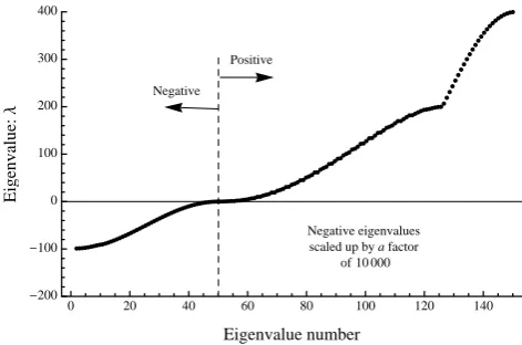
The numerical properties of a linear system are largely de-termined by the distribution of eigenvalues associated with the matrix, and in particular by the condition number. In the present example, withN=50 andh=0.02, we plot the dis-tribution of the eigenvaluesλfor the standard Stokes system, Eq. (51), in Fig. 4, and for the reformulated Stokes system, Eq. (58), in Fig. 5. Note the presence of both negative and positive eigenvalues in Fig. 4, indicating an indefinite matrix in the standard Stokes system, while all eigenvalues in Fig. 5 are positive, indicating a positive-definite matrix.
From the eigenvalue distribution, the condition number for the standard Stokes system is given by
κ (AS)=
Max|λ(AS)|
Min|λ(AS)|
=1.65×10⁸, (61)
and for the reformulated Stokes system by κ (ARS)=
Maxλ(ARS)
Minλ(ARS)
=4.60×10³. (62)
0.0 0.2 0.4 0.6 0.8 1.0
0.20
0.15
0.10
0.05 0.00
Transformed vertical coordinate: z'
Horizontal
velocity:
u
Fig. 3. Horizontal velocity componentu z0
for the case of basal in-clinationθ=18◦and basal friction parameterη=18, correspond-ing to a basal slip parameterγ=10%. The exact solution, from Eq. (39), is shown by the solid line. Discrete points from numer-ical solutions withh=0.02 for the standard Stokes and the refor-mulated Stokes cases are shown dotted. The two cases cannot be distinguished visually.
Positive
Negative
0 20 40 60 80 100 120 140
200
100 0 100 200 300 400
Eigenvalue number
Eigenvalue:
Λ
Negative eigenvalues scaled up by a factor
of 10 000
Fig. 4. The eigenvalue spectrum for the standard Stokes system, Eq. (51). Note that negative eigenvalues have been greatly amplified for clarity.
expect to see significant numerical errors in comparison with the reformulated Stokes system as one goes to higher resolu-tions, although this is not yet evident in Fig. 3.
Large problems, particularly multi-dimensional ones, are solved by iterative methods. The iterative method of choice for symmetric systems, as in this case, is typically one of sev-eral possible Krylov subspace methods. The simpler Krylov methods typically require definite matrices. Indefinite sys-tems, on the other hand, require special methods (Paige and Saunders, 1975; Fletcher, 1976). Furthermore, the conver-gence of Krylov subspace methods depends on the condition number (Saad, 2003). From this we could infer that the re-formulated Stokes system might be much easier to solve than
0 10 20 30 40 50
0 50 100 150 200 250
Eigenvalue number
Eigenvalue:
Λ
Fig. 5. The eigenvalue spectrum for the reformulated Stokes sys-tem, Eq. (58).
0 20 40 60 80 100 120 140
0 2 4 6 8 10
Iteration number
Horizontal
velocity
error
Fig. 6. Conjugate gradient convergence history for the reformulated Stokes system (solid line) and the standard Stokes system (dashed line) for a small problem (N=50,h=0.02).
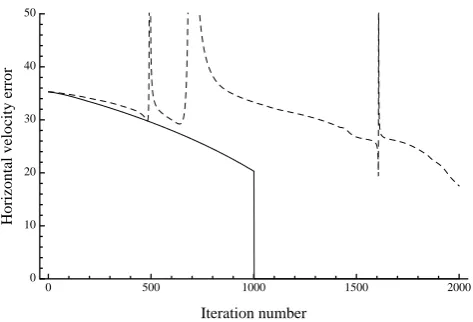
the standard Stokes saddle-point system. We shall illustrate this by looking at the iterative convergence of the two for-mulations when using the conjugate gradient method (Saad, 2003), a prominent Krylov subspace method, even though this method is prone to break down for indefinite problems due to a possible division by zero or a near zero. The itera-tion is initiated with all unknowns set to unity. We plot the convergence history for the two different cases in Fig. 6 for a small problem, N=50, and in Fig. 7 for a much larger problem,N=1000. In all cases we plot the horizontal ve-locity error, i.e., the L2-norm of the difference between the horizontal velocity solution and the exact horizontal velocity from Eq. (39), as a function of the iteration number. The ini-tial error is approximately 8 and 35 for the small and large problem, respectively.
0 500 1000 1500 2000 0
10 20 30 40 50
Iteration number
Horizontal
velocity
error
Fig. 7. Conjugate gradient convergence history for the reformulated Stokes system (solid line) and the standard Stokes system (dashed line) for a relatively large problem (N=1000,h=0.001).
standard Stokes system the corresponding error (at about it-eration 150) is on the order of 10−4.
In the absence of round-off error the conjugate gradient method gives the exact answer inN steps, whereN is the order of the system. This can be seen in Figs. 6 and 7 for the reformulated Stokes case, where the method effec-tively terminates in 50 and 1000 steps, respeceffec-tively. For very large problems, and particularly for multi-dimensional problems, it is not feasible to carry on the calculation for that many steps and the method becomes simply an iterative scheme whose convergence depends on the condition num-ber. Indeed, viewed in this way we see that the reformulated Stokes system converges significantly faster than the stan-dard Stokes system. Moreover, the convergence of the con-jugate gradient method for the standard Stokes system can break down due to its being an indefinite system. We observe breakdowns in the vicinity of iteration 80 and 125 in Fig. 6 for the small problem, and in the vicinity of iteration 500, 700, and 1600 in Fig. 7 for the larger problem. Although the method recovers and convergence resumes, it does so with a larger error. In fact, for the larger problem, the reformu-lated system ends up with an error of order 10−12after about 1000 iterations, while the standard Stokes system continues to converge very slowly and eventually ends up with a much larger error of about 10−3after 4000 iterations.
6 New Euler-Lagrange equations for the reformulated Stokes system
It is of interest to obtain the partial differential equations that characterize the reformulated Stokes system, if only to com-pare them with the standard Stokes system, Eqs. (9–14). For this we need to derive the Euler-Lagrange equations associ-ated with the reformulassoci-ated Stokes action, which we do next. Taking the variation of the action, Eq. (26), as detailed in
DPL10, and making use of Eqs. (21) and (24), we obtain δA0RS=RVdV δGn ε˙RS2 +RVdV δu(i)ρg∂x∂zs
(i) +R
S(b)dSδu
(b) (i)
h
βu(b)(i)+βw(b)n +u(b)(j )∂x∂zb
(j )
∂zb
∂x(i)
i
. (63)
Note that this is linear in the velocity perturbations δu(i), δu(b)(i), and implicitly inδu(s)(i)also. Recall that the
vari-ational principle, i.e., Eq. (8), implies that the variation of the action, Eq. (63), must vanish for arbitrary velocity per-turbations. Therefore, Eq. (63) must now be manipulated into a form such that the integrands in the volume and sur-face integrals are linear functions of the velocity perturba-tions themselves. Since the velocity perturbaperturba-tions are arbi-trary, the coefficients multiplying each of the velocity pertur-bations must vanish, and this gives the required set of Euler-Lagrange equations and also the associated natural boundary conditions. The manipulations required to put Eq. (63) into this form are rather complicated. We do this in Appendix A, and obtain
δA0RS= −
Z
V
dV δu(i)
∂τ˜
(i)j ∂xj
+ ∂
∂x(i)
Z zs
z
dz0∂τ˜z(j ) ∂x(j )
(64)
− ˜τz(j )(s)n(s)(j ) s
1+ ∂zs
∂x(i) ∂zs ∂x(i)
−ρg ∂zs
∂x(i)
#
+
Z
S(s)
dS δu(s)(i)
˜
τ(i)jn(s)j − ˜τz(j )n(s)(j ) ∂zs ∂x(i)
−n(s)(i)τ˜z(j )(s)n(s)(j ) s
1+ ∂zs
∂x(i) ∂zs ∂x(i)
!
+
Z
S(b)
dS δu(b)(i)
˜
τ(i)jn(b)j +βu (b) (i) +βw(b)n +βu(b)(j )∂x∂zb
(j )
+ ˜τz(j )n(b)(j )
∂zb
∂ x(i)
+n(b)(i)τ˜z(j )(s)n(s)(j )q1+ ∂zb
∂x(i)
∂zb
∂x(i)
−q1+ ∂zs
∂x(i)
∂zs
∂x(i)
,
where
˜
τ(i)j=µn(ε˙2RS)
22∂u∂x+∂v
∂y
∂u ∂y+
∂v ∂x
∂u ∂z+
∂w(u(i))
∂x
∂u ∂y+
∂v ∂x
2∂u∂x+2∂v∂y ∂v∂z+∂w(u(i))
∂y
,(65)
and where Eq. (23) and Eqs. (20) or (21) define ε˙2RS and w u(i), respectively. The two-dimensional vectors
com-posed of the horizontal components of the unit vectors at the boundaries, i.e.,n(s)(i), n(b)(i), are defined in the Appendix. Thus, the Euler-Lagrange equations are given by
∂τ˜(i)j ∂xj
+
∂
∂x(i)
Z zs
z
dz0∂τ˜z(j ) ∂x(j )
− ˜τz(j )(s)n(s)(j ) (66) s
1+ ∂zs
∂x(i) ∂zs ∂x(i)
#
=ρg ∂zs ∂x(i)
The associated free-stress upper surface boundary condition is
˜
τ(i)jn(s)j − ˜τz(j )n(s)(j ) ∂zs ∂x(i)
−
h
n(s)(i)τ˜z(j )(s)n(s)(j ) (67) s
1+ ∂zs
∂x(i) ∂zs ∂x(i)
#
=0,
and the generalized basal boundary condition becomes
˜
τ(i)jn(b)j +βu (b) (i)+
βw(b)n +βu(b)(j ) ∂zb ∂x(j )
+ ˜τz(j )n(b)(j )
∂z
b ∂x(i)
(68)
+ "
n(b)(i)τ˜z(j )(s)n(s)(j )
s
1+ ∂zb
∂x(i) ∂zb ∂x(i)
− s
1+ ∂zs
∂x(i) ∂zs ∂x(i)
!#
=0.
As noted earlier, we may setβwn(b)=0 in Eq. (68) except
possibly under unusual circumstances. These are the partial differential equations and boundary conditions that constitute the reformulated Stokes problem. The basal boundary condi-tions include sliding along a rigid bed as well as a generalized floating boundary condition that may, for example, include conditions at the base of an ice shelf. The above equations are very similar to the corresponding Blatter-Pattyn equa-tions (see DPL10) except for extra terms, which we enclose in square brackets for emphasis. These extra terms, in effect, convert the Blatter-Pattyn model into the full-Stokes prob-lem.
7 Summary and conclusions
We have presented a reformulation of the full Stokes problem for ice sheets that converts it from the stan-dard constrained minimization formulation in six variables (u,v,w,P ,3s,3b) into an unconstrained minimization in
only two variables (u,v). This not only reduces the size of the problem but makes the problem much more tractable numerically. Instead of the original indefinite saddle point problem we obtain a positive-definite minimization or opti-mization problem that is directly amenable to a number of ef-ficient solution techniques. In this respect, the reformulated problem is similar to the first-order or Blatter-Pattyn approx-imation, but without the associated approximation errors. An important byproduct of the present formulation is the fact all boundary conditions are already incorporated in the action functional, thereby avoiding many problematic issues with the implementation of boundary conditions in practical mod-els. As an aside, note that this work provides a further exam-ple of the usefulness of the fundamental action princiexam-ple for ice sheets presented in DPL10 and DPL11.
On the negative side, the new system matrix is less sparse and may impose additional continuity requirements on the approximating space, as can be seen from the presence of integrals and (effectively) fourth-order horizontal velocity derivatives in Eq. (66). Note, however, that due to the non-linearity of the problem in general, it might be expected that
the JFNK (Jacobian-Free-Newton-Krylov) method of Knoll and Keyes (2004) will be the preferred solution method, in which case only the functional, Eq. (22) or (26), is required (i.e., the system matrix is never actually formed) and so only second-order horizontal velocity derivatives are needed.
We have noted many advantageous properties of the re-formulated Stokes system compared to the standard Stokes system. We illustrate some of these properties by means of a simple linear two-dimensional ice sheet problem that is re-ducible to a one-dimensional representation. This simplified problem demonstrates better conditioning and convergence for the reformulated system compared to the standard Stokes system. This is encouraging for the application of the present method to more general problems. At this point it is not possible to conclude how computational costs will compare. This question is beyond the scope of the present paper and can only be answered when the method is implemented and evaluated in realistic, three-dimensional problems. In short, the proposed reformulation isn’t likely to solve every prob-lem with full-Stokes modeling, but it is hoped it will amelio-rate many of them and will lead to new directions in ice sheet modeling.
Appendix A
Deriving the Euler-Lagrange equations for the reformulated Stokes problem
A1 Preliminaries
We shall be making frequent use of the following two results: (a) Interchanging the order of integration,
Zb
a
dx g z0,x
Z x
a
dy h z00,y
=
Z b
a
dy h z00,y
Zb
y
dx g z0,x
. (A1)
We have introduced dummy variables z0,z00 as a reminder that variables other thanx,ymay be present. A useful special case is given wheng z0,x=1, as follows
Z b
a dx
Z x
a
dy h z00,y=
Z b
a
dy (b−y)h z00,y. (A2)
(b) Leibniz’s Theorem,
∂ ∂x
Z b(x)
a(x)
dy h z0,x,y=
Z b(x)
a(x)
dy ∂h z 0,x,y
∂x (A3)
+h z0,x,b(x)∂b(x) ∂x −h z
0
A2
The gravity term in the initial form of the reformulated action, Eq. (22)
The gravity term in Eq. (22) contributes to the forcing terms in the Stokes equations. Leaving out the constant factorρg and making use of Eq. (21), it may be usefully simplified as follows
Z
V
dV w u(i)=
Z
V
dV w(b)n −
Z V dV ∂ ∂x(i) Z z zb
u(i)dz0,(A4)
where, making use of Leibniz’s theorem, the last term on the right hand side becomes
Z V dV ∂ ∂x(i) Z z zb
dz0u(i)=
Z
A dA
Z zs
zb dz ∂ ∂x(i) Z z zb
dz0u(i)
(A5) = Z A dA
Z zs
zb
dz Z z
zb
dz0∂u(i) ∂x(i)
−
Z
A dA
Z zs
zb
dz u(b)(i) ∂zb ∂x(i)
.
Note that Arepresents the cross-sectional area at constant z; dA=dx dyis the element of area in this cross-section. Now, making use of Eq. (A2) and temporarily introducing
˜
ui=(u, v,0)T, an extended version ofu(i), we have Z V dV ∂ ∂x(i) Z z zb dz0u(i)=
Z
A
dA Z zs
zb dz
(zs−z)
∂u(i)
∂x(i)
−u(b)(i) ∂zb ∂x(i) (A6) = Z V
dV (zs−z) ∂u˜i ∂xi
−
Z
A
dA(zs−zb)u(b)(i) ∂zb ∂x(i)
.
Using the chain rule and applying Gauss’ theorem, we finally obtain Z V dV ∂ ∂x(i) Z z zb
dz0u(i)=
Z V dV −u(i) ∂zs ∂x(i)
+∂ (zs−z)u˜i ∂xi (A7) − Z A
dA(zs−zb)u(b)(i) ∂zb ∂x(i)
= −
Z
V dV u(i)
∂zs ∂x(i)
+
Z
S(b)
n(b)(i)dS (zs−zb)u(b)(i)−
Z
A
dA(zs−zb)u(b)(i) ∂zb ∂x(i)
= −
Z
V dV u(i)
∂zs ∂x(i)
.
Here,n(b)(i) represents a two-dimensional vector composed of the horizontal components of the basal unit vector given by Eq. (16). Note that we use the fact that the surface element dS=dA
q
1+∂zb∂x(i)∂zb∂x(i)at the basal surface. The
same relations hold at the upper surface with corresponding changes in notation. This last equation, Eq. (A7), together with Eq. (A4) may now be used to obtain Eq. (25), and hence the simpler form of the action, Eq. (26).
A3
Derivations leading to the Euler-Lagrange equations There now remain two terms in Eq. (63) that need to be ma-nipulated into the required form, namely,
I1=
Z
V dV δGn
˙
ε2RS
and I2=
Z
V
dVρgδu(b)(i) ∂zb ∂x(i)
.
The first term,I1, is by far the most complicated and we shall
deal with it first. To do this we shall temporarily assume that the vertical velocity is an independent variable, as in the stan-dard Stokes model, and therefore retain a three-dimensional velocity in the formui∈
u(i),w . However, from Eqs. (19)
and (21), and noting thatδw(b)n =0, we have δw= − ∂
∂x(i)
Z z
zb
δu(i)dz0,δw(b)=δu(i) ∂zb ∂x(i)
. (A8)
Following the procedures in DPL10, we obtain I1=
Z
V dV δGn
˙
ε2RS = Z
V dVτ˜ij
∂δui ∂xj
=I11+I13+I13, (A9)
where I11= −
Z
V dV δui
∂τ˜ij ∂xj
, (A10)
I12=
Z
S(s)
dS δu(s)i τ˜ijn(s)j ,
I13=
Z
S(b)
dS δu(b)i τ˜ijn(b)j ,
and
˜
τij=µn(ε˙RS2 )
22∂u∂x+∂v
∂y ∂u ∂y+ ∂v ∂x ∂u ∂z+ ∂w ∂x ∂u ∂y+ ∂v ∂x
2∂u∂x+2∂v∂y ∂v∂z+∂w
∂y ∂u ∂z+ ∂w ∂x ∂v ∂z+ ∂w ∂y 0 . (A11)
The basal surface integralI13is the simplest; where, making
use of Eq. (A8), it may be rewritten as follows I13 =RS(b)dS δu
(b)
(i)τ˜(i)jn(b)j +
R
S(b)dS δw(b)τ˜z(j )n(b)(j )
=R
S(b)dS δu
(b) (i)
˜
τ(i)jn(b)j +∂x∂zb
(i) ˜
τz(j )n(b)(j )
. (A12)
The upper surface integralI12is more complicated. It may
be expanded and rewritten as follows I12=
Z
S(s)
dS δu(s)(i)τ˜(i)jn(s)j +I121. (A13)
Making use of Leibniz’s theorem and Eq. (A8), the integral I121becomes
I121=
Z
S(s)
dS δw(s)τ˜z(j )n(s)(j ) (A14)
= − Z
S(s)
dSτ˜z(j )n(s)(j )
Z zs
zb
dz0∂δu(i) ∂x(i)
+δu(s)(i) ∂zs ∂x(i)
−δu(b)(i) ∂zb
∂x(i)
= −
Z
S(s)
dS δu(s)(i)τ˜z(j )n(s)(j ) ∂zs ∂x(i)
where I1211= −
Z
S(s)
dSτ˜z(j )n(s)(j )
Z zs
zb
dz0∂δu(i) ∂x(i)
, (A15)
I1212=
Z
S(s)
dS δu(b)(i)τ˜z(j )n(s)(j ) ∂zb ∂x(i)
.
Finally, the volume integralI11becomes
I11= −
Z
V
dV δu(i) ∂τ˜(i)j
∂xj −
Z
V
dV δw∂τ˜z(j ) ∂x(j )
(A16)
= −
Z
V
dV δu(i) ∂τ˜(i)j
∂xj + Z V dV ∂ ∂x(i) Z z zb
δu(i)dz0
∂τ˜
z(j ) ∂x(j )
= − Z V dV δu(i)
∂τ˜(i)j ∂xj
+δu(b)(i) ∂zb ∂x(i)
∂τ˜z(j ) ∂x(j )
+ Z V dV Z z zb ∂δu(i) ∂x(i) dz0 ∂τ˜ z(j ) ∂x(j )
= −
Z
V
dV δu(i) ∂τ˜(i)j
∂xj
+I111+I112,
where again we have used Leibniz’s theorem and Eq. (A8), and where
I111= −
Z
V
dV δu(b)(i) ∂zb ∂x(i)
∂τ˜z(j ) ∂x(j )
, (A17)
I112=
Z V dV Z z zb ∂δu(i) ∂x(i) dz0 ∂τ˜ z(j ) ∂x(j ) .
The last integral,I112, may be put in the appropriate form by
interchanging the order of integration, as follows I112=
Z
A dA
Z zs
zb
dz∂τ˜z(j ) ∂x(j )
Z z
zb
dz0∂δu(i) ∂x(i) (A18) = Z A dA
Z zs
zb
dz∂δu(i) ∂x(i)
Z zs
z
dz0∂τ˜z(j ) ∂x(j )
=
Z
V
dV ∂δu(i) ∂x(i)
Z zs
z
dz0∂τ˜z(j ) ∂x(j )
.
Now, temporarily expressing the velocity perturbation as a three-dimensional vector, δuj=(δu,δv,0)T, and applying
Gauss’ theorem, we obtain I112=
Z
V
dV ∂δuj ∂xj
Z zs
z
dz0∂τ˜z(i) ∂x(i) (A19) = Z V dV ∂ ∂xj δuj
Zzs
z
dz0∂τ˜z(i) ∂x(i)
−
Z
V
dV δuj
∂ ∂xj
Z zs
z
dz0∂τ˜z(i) ∂x(i)
=
Z
S(b)
dS δu(b)(j )n(b)(j )
Zzs
zb
dz0∂τ˜z(i) ∂x(i)
−
Z
V
dV δu(j )
∂ ∂x(j )
Z zs
z
dz0∂τ˜z(i) ∂x(i)
.
Note that integralsI2andI111are basically of the same form.
Combining them, and noting from Eq. (16) that∂zb∂x(i)= n(b)(i)q1+∂zb∂x(i)∂zb∂x(i), we obtain
I3=I2+I111=
Z
V
dV δu(b)(i)
ρg−∂τ˜z(j )
∂x(j )
∂z b ∂x(i) (A20) = Z V
dV n(b)(i)δu(b)(i)
ρg−∂τ˜z(j )
∂x(j )
s 1+ ∂zb
∂x(i) ∂zb ∂x(i)
=
Z zs
zb
dz Z
A
dA n(b)(i)δu(b)(i)
ρg−∂τ˜z(j )
∂x(j )
s 1+ ∂zb
∂x(i) ∂zb ∂x(i)
.
Now, noting thatdS=dA q
1+∂zb∂x(i)∂zb∂x(i) on the
basal surface, and carrying through the integration with re-spect toz, this takes the final form
I3=
Z zs
zb
dz Z
S(b)
dS n(b)(i)δu(b)(i)
ρg−∂τ˜z(j )
∂x(j )
(A21)
=
Z
S(b)
dS δu(b)(i)n(b)(i)
ρg (zs−zb)−
Z zs
zb
dz∂τ˜z(j ) ∂x(j )
.
There are only two integrals left,I111 andI112. Converting
from∂zb∂x(i)ton(b)(i), as before, we obtain I112=
Z
S(s)
dS δu(b)(i)τ˜z(j )n(s)(j ) ∂zb ∂x(i) (A22) = Z S(b)
dS n(b)(i)δu(b)(i)τ˜z(j )(s)n(s)(j ) s
1+ ∂zb
∂x(i) ∂zb ∂x(i)
,
where, since the integrand is a function of horizontal position x(i)only, it is permissible to switch the surface of integration
from the upper to the basal surface. For the last integral, mak-ing use of the fact thatdS=dA
q
1+∂zs∂x(i)∂zs∂x(i)on
the upper surface, we have I111= −
Z
S(s)
dSτ˜z(j )(s)n(s)(j ) Z zs
zb
dz0∂δu(i) ∂x(i)
(A23)
= −
Z
A
dAτ˜z(j )(s)n(s)(j ) s
1+ ∂zs
∂x(i) ∂zs ∂x(i)
Z zs
zb
dz0∂δu(i) ∂x(i)
= −
Z
V
dVτ˜z(j )(s)n(s)(j ) s
1+ ∂zs
∂x(i) ∂zs ∂x(i) ∂δu(i) ∂x(i) .
Now, applying the chain rule and Gauss’ theorem, we obtain the final form,
I111= − Z
V
dV ∂
∂x(i) δu(i)τ˜ (s) z(j )n
(s) (j )
s 1+ ∂zs
∂x(i) ∂zs ∂x(i) ! (A24) + Z V
dV δu(i) ∂ ∂x(i)
˜
τz(j )(s)n(s)(j ) s
1+ ∂zs
∂x(i) ∂zs ∂x(i) ! = − Z S(s)
dS n(s)(i)δu(s)(i)τ˜z(j )(s)n(s)(j ) s
1+ ∂zs
∂x(i) ∂zs ∂x(i) − Z S(b)
dS n(b)(i)δu(b)(i)τ˜z(j )(s)n(s)(j ) s
1+ ∂zs
∂x(i) ∂zs ∂x(i) + Z V
dV δu(i) ∂ ∂x(i)
˜
τz(j )(s)n(s)(j ) s
1+ ∂zs
∂x(i) ∂zs ∂x(i)
Since everything is now in the required form, we may com-bine Eqs. (A9)–(A24) to obtain Eq. (64) in Sect. 6.
Acknowledgements. Funding for this work was provided by the
Climate Modeling program in the US Department of Energy’s Office of Science (Biological and Environmental Research). Los Alamos National Laboratory is operated under the auspices of the National Nuclear Security Administration of the US Department of Energy under Contract No. DE-AC52-06NA25396.
Edited by: D. M. Holland
References
Benzi, M., Golub, G. H., and Liesen, J.: Numerical solution of saddle point problems, Acta Numerica, 14, 1–137, 2005. Blatter, H.: Velocity and stress fields in grounded glaciers: A simple
algorithm for including deviatoric stress gradients, J. Glaciol., 4, 333–344, 1995.
Brezzi, F. and Fortin, M.: Mixed and hybrid finite element meth-ods, Vol. 15 (Springer Series in Computational Mathematics), Springer, New York, 350 pp., 1991.
Dukowicz, J. K., Price, S. F., and Lipscomb, W. H.: Consistent approximations and boundary condition for ice sheet dynamics from a principle of least action, J. Glaciol., 56, 480–496, 2010. Dukowicz, J. K., Price, S. F., and Lipscomb, W. H.: Incorporating
arbitrary basal topography in the variational formulation of ice sheet models, J. Glaciol., 57, 461–467, 2011.
Elman, H. C., Silvester, D. J., and Wathen. A. J.: Finite Elements and Fast Iterative Solvers, Oxford University Press, 414 pp., 2005.
Fletcher, R.: Conjugate gradient methods for indefinite systems, in: Numerical Analysis, edited by: Watson, G., Springer-Verlag (Se-ries: Lecture Notes in Mathematics), 73–89, 1976.
Greve, R. and Blatter, H.: Dynamics of Ice Sheets and Glaciers, Springer-Verlag, Berlin, 287 pp., 2009.
Hindmarsh, R. C. A.: Modelling the dynamics of ice-sheets, Prog. Phys. Geog., 17, 391–412, 1993.
Knoll, D. A. and Keyes, D. E.: Jacobian-free Newton–Krylov meth-ods: A survey of approaches and applications, J. Comput. Phys., 193, 357–397, 2004.
Nocedal, J. and Wright, S.: Numerical Optimization, Second Ed., Springer, 664 pp., 2006.
Paige, C. C. and Saunders, M. A.: Solution of sparse indefinite sys-tems of linear equations, SIAM J. Numer. Anal., 12, 617–629, 1975.
Pattyn, F.: A new three-dimensional higher-order thermomechani-cal ice sheet model: Basic sensitivity, ice stream development, and ice flow across subglacial lakes, J. Geophys. Res., 108(B8), 2382, doi:10.1029/2002JB002329, 2003.
Pattyn, F.: Investigating the stability of subglacial lakes with a full Stokes ice-sheet model, J. Glaciol., 54, 353-361, 2008.
Pattyn, F., Perichon, L., Aschwanden, A., Breuer, B., de Smedt, B., Gagliardini, O., Gudmundsson, G. H., Hindmarsh, R. C. A., Hubbard, A., Johnson, J. V., Kleiner, T., Konovalov, Y., Mar-tin, C., Payne, A. J., Pollard, D., Price, S., R¨uckamp, M., Saito, F., Soucek, O., Sugiyama, S., and Zwinger, T.: Benchmark experiments for higher-order and full-Stokes ice sheet models (ISMIPHOM), The Cryosphere, 2, 95-108, doi:10.5194/tc-2-95-2008, 2008.
Saad, Y.: Iterative methods for sparse linear systems, Second Ed., SIAM, 528 pp., 2003.
Schoof, C.: Coulomb friction and other sliding laws in a higher order glacier flow model, Math. Mod. Meth. Appl. S., 20, 157– 189, 2010.
Van der Veen, C. J. and Whillans, I. M.: Force Budget: I. Theory and Numerical Methods, J. Glaciol., 35, 53–60, 1989.