Control Systems Design Based on Classical Dynamics

Published online September 30, 2014 (http://www.sciencepublishinggroup.com/j/acis) doi: 10.11648/j.acis.20140205.12

ISSN: 2328-5583 (Print); ISSN: 2328-5591 (Online)

Control systems design based on classical dynamics

Wang Funing

1

, Kai Pingan

2

1

Ningdong Power Plant, Gouhua Power Group, Ningdong town, Ningxia, P. R. C.

2

Energy Research Institute, Development and Reformation Committee of State, Beijing, P. R. C.

Email address:

[email protected] (Wang Funing), [email protected] (Kai Pingan)

To cite this article:

Wang Funing, Kai Pingan. Control Systems Design Based on Classical Dynamics. Automation, Control and Intelligent Systems. Vol. 2, No. 5, 2014, pp. 81-86. doi: 10.11648/j.acis.20140205.12

Abstract:

The paper presents unity between control systems and classical dynamics. A state observer is constructed based on uniformly accelerated motion. It is known F = ma _{in Newtonian motion equation is considered as a control input force which} functions on the controlled plant process. The designed control system is of good robust performance.

Keywords:

Uniformly Accelerated Motion, Newtonian Mechanics, State Observer, Kalman Filter, Robust Performance

1. Introduction

Design control systems in modern control theory always needs a mathematics model of controlled plant , however the model is not exactly obtained and the model is uncertain in general, these limits led to the poor control system performance.

The paper designs a control system based on Classical dynamics without exact plant model, and the systems are of good robust performances.

2. State Observer Based on Uniformly

Accelerated Motion

When a motion (/response) velocity of controlled plant process (/ body) is greatly less than velocity of light, we can describe its motion using uniformly acceleration motion:

2 0 0 0.5 S=S +V t+ at

0 .

S =V = V + a t (1)

.. .

S= =V a

where S V a, , are respectively the position, velocity and acceleration of the body/process motion.

Assume a controlled second system with the random disturbance ( )v t :

( , , ( )) y= f y y v t +bu

ɺɺ ɺ (2)

the system in state space is:

2 1

.

y =y

1 2 2

.

( , , ( ))

y = f y y v t +bu (3)

1

y

=

y

For a controlled plant process, assumingz(1),z(2),⋯,z(k), the k measurement output data are obtained from the controlled plant output y k( ) , sample(/control) period is ts, the measurement equation is

)

(

)

(

)

(

k

y

k

v

k

z

=

+

, (4)

where: 2

2 [ ( )]

[ ( )] 0

E k r

E v k

v =

= )

(k

v _{is white noise}, we can estimate the controlled plant

output y k( ) using Exp. (1) based on z(1),z(2),⋯,z(k), when

t

s is very short,

2 ˆ( ) ˆ( 1) ˆ( 1) 0.5 ˆ( 1) ˆ( ) ˆ( 1) ˆ( 1)

ˆ( ) ˆ( 1)

s s

s

y k y k t y k t y k

y k y k t y k

y k y k

= − + − + −

= − + −

= −

ɺ ɺɺ

ɺ ɺ ɺɺ

ɺɺ ɺɺ

(5)

let ^ ˆ( ) ˆ ( ) ( ) ˆ( ) y k

Y k y k

y k     =      ɺ ɺɺ and 2 1 2 0 1

0 0 1

s s s t t t φ     =_{ }     (6)

Exp. (5) can be written as:

^ ^

( ) ( 1)

Y k =φY k− (7)

To improve estimate accuracy, the compensating for random disturbance is into acceleration estimate ˆ( )ɺɺy k :

ˆ

( )

(

ˆ

1)

(

1)

y k

=

y k

− +

w k

−

ɺɺ

ɺɺ

(8)

where：E[w(k)]=0, ₁ 2

)] ( [w k r

E =

Exp.(7) becomes:

^ ^

( ) ( 1) ( 1)

Y k =φY k− + Γw k− (9) where：

[

]

T 1 0 0 = Γ

measurement equation (4) is written as:

^

( ) ( ) ( )

z k =c Y k +v k , (10)

where:c=[1 0 0]

Kalman filter theory can be used for state equation (9) and measurement equation(10),

φ

and Γ are constant matrixes, meet rank( , )

φ

Γ =n , rank( , )φ c =n , so the system is completely controllable and observable in Kalman filter theory( the proof is given the following lemma), when

t

_s is

very short and filtering time is very long, the covariance

matrix,

lim ( )

k→∞P k =P,

gain matrix

( )

k

Lim K k K

→∞ = ,

( ) [ , , ]T

K k → =K

α β γ

.

We have the following time discrete observer to an unknown controlled plant:

2

ˆ( ) ˆ( 1) ˆ( 1) 0.5 ˆ( 1) ( ( ) ˆ( 1))

ˆ( ) ˆ( 1) ˆ( 1) ( ( ) ˆ( 1))

ˆ( ) ˆ( 1) ( ( ) ˆ( 1))

s s s

s s

s

y k y k t y k t y k t z k y k y k y k t y k t z k y k

y k y k t z k y k

α β γ  _{= − + − + − + − −}  = − + − + − −   = − + − −  ɺ ɺɺ ɺ ɺ ɺɺ ɺɺ ɺɺ (11)

F=ma in the classical dynamics. Referencing Exp.(3), the control input u _{is considered as a force which functions} on the controlled plant, u=F, and a=

θ

u , where F is the force and a _{is the acceleration.}

As

ɺɺ

y k

ˆ

( )

=

( ( )

y k

ˆ

ɺ

−

y k

ˆ

ɺ

(

−

1)) /

t

s is an estimate to the

acceleration of the system,

ˆ

( )

( ( )

ˆ

ˆ

(

1)) /

_s

(

1)

y k

=

y k

−

y k

−

t

=

θ

u k

−

ɺɺ

ɺ

ɺ

so,

ˆ

( )

ˆ

(

1)

(

1)

s

y k

ɺ

=

y k

ɺ

− +

t u k

θ

−

Relate Exp.(11),

ˆ

( )

ˆ

(

1)

s

ˆ

(

1)

s

( (

1)

ˆ

(

1))

y k

ɺ

=

y k

ɺ

− +

t y k

ɺɺ

− +

β

t z k

− −

y k

−

, we

have

ˆ( ) ˆ( 1) sˆ( 1) s( ( 1) ˆ( 1)) s ( 1) y kɺ =y kɺ − +t y kɺɺ − +βt z k− −y k− +t u kθ −

Exp.(11）becomes:

2

ˆ( ) ˆ( 1) ˆ( 1) 0.5 ˆ( 1) ( ( ) ˆ( 1))

ˆ( ) ˆ( 1) ˆ( 1) ( ( ) ˆ( 1)) ( 1) ˆ( ) ˆ( 1) ( ( ) ˆ( 1))

s s s

s s s

s

y k y k t y k t y k t z k y k

y k y k t y k t z k y k t u k

y k y k t z k y k

α β θ γ  _{= − + − + − + − −}  = − + − + − − + −   = − + − −  ɺ ɺɺ ɺ ɺ ɺɺ ɺɺ ɺɺ (12)

Exp.(12) is a time discrete observer with control input

u

for the control system (3)

Using the transformation

2 2

0.5

I

+

At

+

A t

=

φ

We have the following time continuous observer of an unknown controlled plant

1 2 2 3 3 ˆ ˆ ( ˆ) ˆ ˆ ( ˆ) ˆ ( ˆ)

y y z y

y y z y u

y z y

α β θ γ  _{= + −}  = + − +   = −  ɺ ɺ ɺ (13)

where

y

ˆ

1

=

y

ˆ

;

2 ˆ ˆ y =yɺ ;

3

ˆ ˆ

y =ɺɺy,

t

_s is sample(/control)

period,

u

is control input to the plant system, l≤ ≤

θ

h,.

l

and

h

are real boundary numbers.

Exp.（13）is the time continuous observer of an unknown

controlled plant with control input

_u

for the control system (3), Exp.（13）is simply called OCICD(Observer with Control

Input based on Classical Dynamics).

Lemma. Discrete systems (9) and (10) are completely controllable and observable.

Proof. The state matrix

φ

is time-invariant, as

t

_s is determined in systems (9), we calculate

2 2

2

0 2 2 ( , ) [ | | ] 0 2

1 1 1

s s s s t t t t φ φ φ     Γ = Γ Γ Γ =_{ }     2 2 2

1 1 1

( , ) [ | | ( ) ] 0 2 0 2 2

T T T T T

s s

s s

c c c c t t

t t φ φ φ     = =_{ }    

( , ) 3

rank

φ

Γ = , rank( , )

φ

c =3; so discrete systems (9) and (10) are completely controllable and observable.

Theorem 1. Time continuous observer system (13) is consistent asymptotic stable.

Proof. We have proved discrete systems (9) and (10) are completely controllable and observable, time discrete observer (12) is obtained by Kalman filter, so time discrete observer（12）is consistent asymptotic stable when α β, and

obtained by transforming time discrete observer (12), so time continuous observer (13) is also consistent asymptotic stable, when

α β

,

and

γ

are rightly selected. From characteristic

equation

sI

−

A

=

s

3

+

α

s

2

+

β

s

+

γ

of time continuous

observer (13), if

0 >

α ,β>0_,γ>0 _and αβ >γ_{, (14)}

then time continuous observer system (13) is consistent asymptotic stable, based on Routh and Hurwitz's stability criterion.

We set

2 3

1 / ,t_s 0.5 /t_s , 0.088 /t_s

α

=

β

=

γ

= (15)

in time continuous observer system (13) based on Exp. (14) and our experience.

Exp. (15) is only related to a sample (/control) period t_s, and independents from a controlled plant.

Theorem 2.

y

ˆ

₃ in time continuous observer system (13) is unbiased estimate value to f x x v t( ,1 2, ( ))in a second order state space model (3) :

Proof. It is known, Kalman filter is an unbiased estimator, time discrete observer (12) and time continuous observer system (13) are the special applications of Kalman filter, and second system (3) is completely controllable and observable, so time discrete observer (12) and time continuous observer system (13) are unbiased estimators to system (3).

Let

3

( ,

1 2

, ( ))

x

=

f x x v t

(16)

System (3) is written as:

1 2

2 3

3 1 2

1

( , , ( )) x x

x x bu

x f x x v t y x

=  

= +  

= 

 ₌

 ɺ ɺ

ɺ

ɺ (17)

Comparing Exp. (17) with Exp. (13):

1 2

2 3

3

1

ˆ ˆ ( ˆ)

ˆ ˆ ( ˆ)

ˆ ( ˆ)

ˆ ˆ

y y z y

y y z y u

y z y

y y α

β θ

γ

 _{= + −}



= + − +

 

= −

 

=



ɺ

ɺ

ɺ

Because time continuous observer system (13) is unbiased estimator to system (3), we have:

1 1

ˆ ,

y → =x y

y

ˆ

₂

→

x

₂,

y

ˆ

₃

→ =

x

₃

f x x v t

( ,

_{1 2}

, ( ))

(18)

We have proven yˆ3 in time continuous observer system (13) is unbiased estimate value to

f x x v t

( ,

_{1 2}

, ( ))

in a second system (16).

We have the following observer system for a controlled plant process with acceleration

a

=

0

:

1 2

ˆ

ˆ

(

ˆ

)

y

ɺ

=

y

+

α

z

− +

y

θ

u

; yˆɺ2 =

β

(z−yˆ) (19)

1 ˆ ˆ

y=y

where

α

=

1 / ,

t

_s

β

=

0.5 /

t

_s2

We have the following observer system for a controlled plant process with varying acceleration

_a

1 ₁

2 2

3 3

4 4

ˆ _{1 0 0 ˆ 0}

ˆ 0 1 0 ˆ 0

ˆ 0 0 1 ˆ

ˆ

0 0 0 0

ˆ

y _y

y y z

y u

y

y y

α α

β β

γ γ λ

θ θ

  _{−    }

  _{    }

−

  _{    } 

= +

  _{−    } 

 

  _{    }

  _{−    }

 

ɺ

ɺ

ɺ

ɺ

(20)

1

ˆ

ˆ

y

=

y

where

α

=

1 / ,

t

s

β

=

0.5 /

t

s2

3

0.088 /

t

_s

γ

=

, 4

0.01 /ts

θ= .

Fig 1. COCD (Controller with Observer based on Classical dynamics).

A controller and control system with OCICD are respectively designed shown in Fig.1 and Fig.3. The position, velocity and acceleration of control system output are negative feedback function in system. The controlled plant is a second order state space model (3), the second order system is of general model in process control system.

The controller of Fig.1 is called as COCD (Controller with Observer based on Classical dynamics), it consists of setting desire system output locus, OCICD and controller output. The control system of Fig.3 is called as CSCOCD (Control System with COCD).

3.1. Setting Desire System Output Locus

The desire system output

y

is designed in COCD,

2

/ (

1)

_r

( ) ;

y

=

R

as

+ + =

bs

G s R

2

( )

1 / /(

1)

r

G s

=

as

+ +

bs

(21)

where

R

is the amplitude of step input,

2

1/

_n

,

2 /

_n

a

=

w

b

=

ς

w

; (22)

n

w

is the undamped natural frequency,

ς

is the damping coefficient.

The desire transient process time T is defined as the time in

which

y

approaches to 0.98*R for the closed loop system, and Tis related to Exp. (22) , (23) and (24).

1

ς

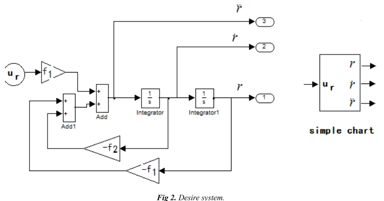
= , w_n=7 /T, (23)

then the desire system is determined, it is configured in state space model shown in Fig,2, f1=1 / ,a f2=b a/ in Fig,2.

Fig 2. Desire system.

3.2. Determining Parameters of OCICD

The sample ts is determined by the sample theory and our

experience:

/ ,

s

t

=

T n

n∈[1000 2000] (24)

where Tis the desire transient process time, the α β, _and

γ

are calculated by Exp. (15).

Fig 3. CSCOCD(Control system with COCD ).

3.3. Controller Output

If the value b in controlled plant state space model (17) is known, let

0 1 2

(

( ,

, ( ))) /

u

=

u

−

f x x v t

b

(25)

then controlled plant state space model (16) is changed to

1 2

2 0

1

x

x

x

u

y

x

=





=





₌



ɺ

ɺ

A suitable

u

₀ is selected, the transform function

G s

_a

( )

( ) [1, 0]

a

G s =

1

2

0 0 1 0

1 /

0 0 0 1

s

s s

−

     

− =

           

  ,

If

f x x v t

( ,

1 2

, ( ))

in controlled plant state space model (3) is uncertain, then the uncertain f x x v t( ,1 2, ( )) including unknown disturbance v t( ) are completely removed. We have

proven that

y

ˆ

3 in time continuous observer system (13) is

unbiased estimate value tof x x v t( ,1 2, ( )) in Theorem 2, so we select K3=1 /b, and

1

(

ˆ

1

)

2

(

ˆ

2

)

3

ˆ

3 0

ˆ

3

/

u

=

K r

−

y

+

K r

ɺ

−

y

−

K y

= −

u

y

b

(26)

where u0=K r1( −yˆ1)+K r2(ɺ−yˆ2).

If controlled plant space model (16) is known, then

b

θ

= ,

K

₃

=

1/ ,

θ

(27)

and K1 andK2 can be obtained by the solution of optimal linear-quadratic Gaussian algorithm(LQG) for the controlled plant space model (3).

If the plant state space model (17) is unknown, assuming

,

l

≤ ≤

b

h

(28)

we set firstly:

(l h) / 2

θ= + , K3=1/θ, K1∈[1 1.5], K2∈[0.5 2] (29)

then we can determine θ,K K K1, 2, 3by several times tests based on the golden section.

It is important to determine desire transient process time T without the mathematics model of controlled plant . Control

engineers must estimate the motion (/response) velocity and completing time of controlled plant process based on analysis and understanding for a controlled plant process, just as the time program to plan a trip, we must estimate velocity and completing time of a vehicle.

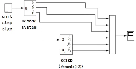
Fig 4. Inspecting the OCICD efficiency.

4. Simulation and Application Examples

with COCD

4.1. Simulation Example

Fig.4 is simulated with Matlab to inspect the OCICD efficiency. The second system transfer function

2

G ( ) 1/ (0.21_p s = s +0.37s+1) is configured as Fig.2, where

1 4.76, 2 1.76,R=1,

f = f = .

T=1(sec),t

_s

=

0.001,

α

=

1000,

500000, 88000000

β

=

γ

= in OCICD.

The simulated curves of OCICD outputs and the second system outputs are shown in Fig.5, the OCICD outputs are very close to the second system outputs, Fig.5 confirms OCICD (13) which is an unbiased estimator to a system.

Fig 5. Comparing outputs of OCICD and the second system.

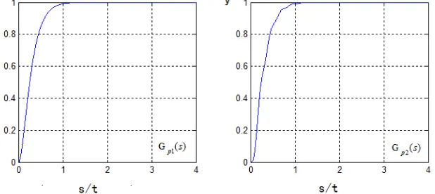
4.2. Application Example

CSCOCD of Fig.3 is used to control the time-varying controlled plant with the transfer function

2 1

G ( )p s =0.8 / (0.21s +0.37s+1) and

2 2

G ( ) 1.3 / (0.06p s = s +0.17s+1) in some steel factory. The same parameters are selected for the

time-varying controlled plants

G ( )

p1

s

and

G ( )

p2

s

:

Fig 6. Outputs of the closed loop system of G ( )p1s and Gp2( )s .

The closed loop system outputs of G ( )p1 s and G ( )p2 s with the same control parameters are shown in Fig.6, and Fig.6.

confirms good robust performance of CSCOCD.

5. Conclusion

(1)The paper designs the control system based on classical dynamics and explains classical dynamics philosophy of the control system design.

(2)The control system is of good robust performance, it can overcome the uncertain of a controlled plant and remove disturbances into the system in the paper. (3)The design of control system needs not an exact

mathematics model of the controlled plant. If we can estimate the values Tin Exp. (24) and l h, in Exp. (29),

we can design the control system without an exact mathematics model of the controlled plant.

References

[1] Kalman, R. E., 'On the general theory of control systems', Ire Transactions On Automatic Control (1959) Volume: 4, Issue: 3, Publisher: Butterworth, London, pp. 110-110.

[2] Kudva, P., Viswanadham, N., Ramakrishna, A., 'Observers for linear systems with unknown inputs', IEEE Trans. Automat. Control, 1980. pp.113~115.

[3] [3] R. E. Kalman, R. S. Bucy, 'New results in linear filtering and prediction theory', J. Basic Eng, 1961 [7]. pp.111-145. [4] Corless. M, Tu.J State/input estimation for a class of uncertain

system system,Automatica, 1998, 34(6); pp.757-764. [5] Jingqing Han, 'Nonlinear State Error Feedback Control',

Control and Decision (Chinese), Vol.10, No.3, Nov., 1994, pp.221-225.