http://www.sciencepublishinggroup.com/j/ajsea doi: 10.11648/j.ajsea.20170603.16
ISSN: 2327-2473 (Print); ISSN: 2327-249X (Online)
Performance Evaluation of Hata-Davidson Pathloss Model
Tuning Approaches for a Suburban Area
Wali Samuel
1, Njumoke N. Odu
2, Samuel Godwin Ajumo
21Department of Electrical/Electronic and Computer Engineering, University of Uyo, Uyo, Nigeria 2
Department of Electrical/Computer Engineering, Port Harcourt Polytechnic, Port Harcourt, Nigeria
Email address:
[email protected] (W. Samuel)
To cite this article:
Wali Samuel, Njumoke N. Odu, Samuel Godwin Ajumo. Performance Evaluation of Hata-Davidson Pathloss Model Tuning Approaches for a Suburban Area. American Journal of Software Engineering and Applications. Vol. 6, No. 3, 2017, pp. 93-98.
doi: 10.11648/j.ajsea.20170603.16
Received: January 3, 2017; Accepted: January 18, 2017; Published: June 23, 2017
Abstract:
In this paper, comparative study of RMSE-base tuning and multi-parameter-based tuning of Hata-Davidson pathloss model for a suburban area is presented. The study was based on field measurement of received signal strength carried out in a suburban area for a GSM (Global System for Mobile communication) network that operates in the 1800MHz frequency band. The results show that multi-parameter-tuned Hata-Davidson model has better prediction accuracy of 98.70720432% and RMSE of 2.177522885 dB as against the RMSE-tuned Hata-Davidson model with prediction accuracy of 97.42722692% and RMSE of 4.256897001dB. However, the RMSE is quite simple and easier to implement even in embedded systems and systems with limited resource.Keywords:
Pathloss, Propagation Model, Hata-Davidson Model, Model Optimisation,Multi-Parameter-Based Tuning Method, RMSE-Base Tuning Method, Least Square Error Method
1. Introduction
Pathloss models are essential in planning wireless network. The models provide mathematical expressions that enable network designers to determine the amount of pathloss that will be experienced by the signal as it transverse the given terrain [1-5]. Basically, a propagation pathloss model predicts the difference between the transmitted power and the receiver power using empirical and deterministic methods or a combination of both. Empirical models, in general, require adjusting some parameters according to field measurements made in a particular environment. Several empirical pathloss models have been given attention for decades due to their accuracy and environmental compatibility. However, peculiarities of these models give rise to high prediction errors when deployed in a different environment other than the one they are initially built for. For instance, [6] provides the error bounds on the efficacy at predicting pathloss for eight widely used empirical pathloss models based on field strength measurements conducted in the VHF and UHF
Hata-Davidson model [12]. The first approach is based on addition or subtraction of the RMSE value whereas the second approach is based on the adjustment of some Hata-Davidson model parameters in such a way as to minimise the sum of square error. The performance of the two tuning approaches are compared in terms of their RMSE and prediction accuracy.
2. Method
The field measurement route is identified with respect to the Cellular Network Base Station (CNBS) selected for the study. Received Signal Strength (RSS) and spatial data (longitude, latitude and altitude) dataset are then collected along the route. Samsung Galaxy S4 mobile phone with Cellmapper android application installed is used to capture and store the RSS and spatial datasets in CSV file. The RSS is converted to the measured pathloss (PL) using the formula [13-15]:
( ) = PBTS + GBTS + GMS – LFC – LAB – LCF – RSS (dBm) (1) where
for each measurement location at a distance d (km)
RSS is the mean Received Signal Strength (RSS) in dBm
PBTS = Transmitter Power (dBm), GBTS = Transmitter
Antenna Gain (dBi), GMS = receiver antenna gain (dBi), LFC =
feeder cable and connector loss (dB), LAB = Antenna Body Loss (dB) and LCF = Combiner And Filter Loss (dB). The
values of these parameters are given as [13]: PBTS = 40 W = 46
dBm, GBTS = 18.15 dBi, GMS = 0 dBi, LFC = 3 dB, LAB = 3 dB, LCF = 4.7 dB. Hence,
( ) = 53.5 (dBm).– RSS (dBm) (2)
Again, the Haversine formula in Eq 3 is used to computer the distances (d) between each measurement point and the base station as follows; = 2 sin + cos( ) cos( ) sin !" !" # (3)
LAT in Radians = ($%& () *+,-++. ∗ 0. 2 )34 (4)
LONG in Radians = ($567 () *+,-++. ∗ 0. 2 )34 (5)
Where LAT1 and LAT2 are the latitude of the coordinates of point1 and point 2 respectively. LONG1 and LONG2 are the longitude of the coordinates of point1 and point 2 respectively. R = radius of the earth = 6371 km; R varies from 6356.752km at the poles to 6378.137 km at the equator d = the distance between the two coordinates Eventually, the distance (d) data is used in the Hata-Davidson model to generate the predicted pathloss. The prediction accuracy of the pathloss model is evaluated with respect to the measured pathloss. The optimised pathloss model is then develop to improve on the prediction accuracy of the Hata-Davidson model. Finally, the prediction accuracy of the optimised pathloss model is compared with the prediction accuracy of the original (un-optimised) Hata-Davidson model. 2.1. Hata-Davidson Propagation Model Hata-Davidson model is one of the extensions or modified versions of Hata model. Particularly, Hata-Davidson is Telecommunications Industry Association (TIA) recommended model following modification to the Hata model to cover a broader range of input parameters. The modification consists of the addition of correction terms to the Hata model. The following equations are used for the computation of the pathloss (in dB) according to the Hata-Davidson model [12]: 89:9_<9=> ?@A= 8 + B<9=> ?@A (6)
Where is the pathloss prediction by the Hata model and is the correction factor introduced by Davidson. The following equations are used for the computation of pathloss (in dB) according to the Hata model: C_8 (DEF9A) = + G ∗ log 4( ) JK L MNO (7)
C_8 (?DFDEF9A) = + G ∗ log 4( ) − Q JK RSMS MNO (8)
C_8 (@TUA/EDE9W) = + G ∗ log 4( ) − X JK Rural (9)
= 69.55 + 26.16 ∗ log 4(J) − 13.82 ∗ log 4(ℎF) − N(ℎ ) (10)
G = 44.9 − 6.55 ∗ log 4(ℎF) (11)
Q = 5.4 + 2 ∗ alog 4 b3 c (12)
X = 40.94 + 4.78 ∗ flog 4(J) g − 18.33 ∗ log 4(J) (13)
N(ℎ ) = f1.1 ∗ log 4(J) − 0.7g ∗ ℎ − f1.56 ∗ log 4(J) − 0.8g (14)
Now, for large city
N(ℎ ) = 8.28 ∗ flog4(1.54 ∗ ℎ ) g − 1.1 f ≤ 200MHz (15) N(ℎ ) = 3.2 ∗ flog 4(11.75 ∗ ℎ ) g − 4.97 f ≥ 400MHz (16)
Where
f is the centre frequency f in MHz d is the link distance in km
is an antenna height-gain correction factor that depends upon the environment
C and D are used to correct the small city formula for suburban and open areas
150 MHz≤ f≤ 1000MHz 30m ≤ ≤ 200m
1m≤ ≤ 10 m 1 km ≤ d ≤ 20km
The following equations are used for the correction factor, introduced by Davidson:
B<9=> ?@A = A(ℎF, ) − R( ) − R (ℎF, ) − R0 (J) − R2 (J, ) (17)
Where
A (, and ( are distance correction factors, (, is base station antenna height correction factor, ( and (, are frequency correction factors.
A (, and ( are distance correction factors, with d in km, in m;
(, is base station antenna height correction factor with d in km, in m;
( and (, are frequency correction factors with f in MHz and d in km.
B<9=> ?@A = A(ℎF, ) − R( ) − R (ℎF, ) − R0 (J) − R2 (J, ) (17) Where
A (ℎF, ) and R ( ) are distance correction factors, R (ℎF, ) is base station antenna height correction factor, R0 (J) andR2 (J, ) are frequency correction factors.
A (ℎF, ) and R ( ) are distance correction factors, with d
in km, ℎF in m;
R (ℎF, ) is base station antenna height correction factor with d in km, ℎF in m;
R0 (J) andR2 (J, ) are frequency correction factors with f in MHz and d in km.
A(ℎF, ) = p
0
0.62317 ( − 20) a0.5 + 0.15log qr
.s c
0.62317 ( − 20) a0.5 + 0.15log qr
.s c
< 20uv 20 < < 64.38uv
20 < < 300uv (18)
S (d) = y 00
0.174(d − 64.38)
d < 20km 20 < d < 64.38km
20 < d < 300km (19) R (ℎF, ) = 0.00784 |log s.s3 | (ℎF− 300) for ℎF< 300 (20)
R0 (J) = b
}4~W@• €••‚ ƒ (21)
R2 (J, ) = „0.112 ~…K† }44b ƒ‡ ( − 64.38) for > 64.38uv (22)
2.2. Performance Analysis of the Models
The statistical performance measures or goodness of fit measures for the Hata-Davidson model are defined as follows: i) The Root Mean Square Error (RMSE) is calculated as follows:
MSE = Š Aa∑> Ž A> Ž Œ ( U9?DEU )(>)− (TEU >•:U )(>) Œ c• (23)
ii) Then, the Prediction Accuracy (PA, %) based on mean absolute percentage deviation (MAPD) or Mean Absolute Percentage Error (MAPE) is calculated as follows:
PA = ‘1 −A ’∑ “Œ”(•–—˜™š–›)(œ) ”(•š–›œžŸ–›)(œ) Œ
” (•–—˜™š–›)(œ) “
>ŽA
>Ž ¡ * 100% (24)
2.3. Model Optimization Process
The parameters of the Hata-Davidson pathloss model were adjusted (optimized) using least square algorithm to fit to measured data using the following process.
1) First, the residual (or error, e) between measured pathloss, and the Hata-Davidson model predicted pathloss is calculated for each location point, i.
¢(>) = ( )(>) - ( )(>) (25)
3) Thirdly, if < 0 then the optimised model is obtained by subtracting RMSE from each otherwise, if ≥ 0 the optimised model is obtained by adding RMSE to each .
3. Results and Discussions
Table 1 gives the measured Received Signal Strength (RSSI), the measured pathloss and the distance of the measurement point from the GSM (Global System for Mobile communication) base station in a suburban area of Uyo, Akwa Ibom state, Nigeria. The GSM network operates in the 1800MHz frequency band.
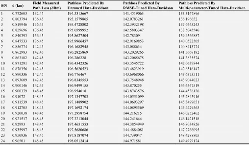
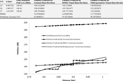
Table 2 and figure 1 show the measure pathloss, the predicted pathloss by untuned Hata-Davidson model, the
predicted pathloss by the RMSE-tuned Hata-Davidson model and the predicted pathloss by the multi-parameter-tuned Hata-Davidson model. The results in table 2 show that the multi-parameter-tuned Hata-Davidson model has the better prediction accuracy of 98.70720432% and RMSE of 2.177522885 dB as against the RMSE-tuned Hata-Davidson model with prediction accuracy of 97.42722692% and RMSE of 4.256897001dB. According to experts, pathloss model with RMSE of less than 6dB is acceptable. In any case, the result shows that the multi-parameter tuning approach may be preferred when more accurate prediction result is required. However, the RMSE is quite simple and easier to implement even in embedded systems and systems with limited resource.
Table 1. The Measured Received Signal Strength (RSSI) and Measured Pathloss and Distance.
S/N d (km) RSSI (dB) Field Measured Path Loss (dBm) S/N d (km) RSSI (dB) Field Measured Path Loss (dBm)
1 0.7726 -79 132.45 14 0.900146 -89 142.45
2 0.8038 -83 136.45 15 0.900379 -95 148.45
3 0.8199 -83 136.45 16 0.91072 -95 148.45
4 0.8297 -83 136.45 17 0.911539 -95 148.45
5 0.8404 -83 136.45 18 0.912705 -95 148.45
6 0.8475 -83 136.45 19 0.920038 -95 148.45
7 0.8568 -89 142.45 20 0.921517 -95 148.45
8 0.8630 -89 142.45 21 0.92993 -95 148.45
9 0.8632 -89 142.45 22 0.935997 -95 148.45
10 0.8713 -89 142.45 23 0.950936 -95 148.45
11 0.8784 -89 142.45 24 0.96501 -95 148.45
12 0.8903 -89 142.45 25 0.983726 -95 148.45
13 0.8936 -89 142.45 26 1.001317 -95 148.45
14 0.9001 -89 142.45 27 1.011593 -97 150.45
Table 2. Measure Pathloss, Predicted Pathloss By Untuned and Tuned Hata-Davidson Models.
S/N d (km) Field Measured Path Loss (dBm)
Pathloss Predicted By Untuned Hata-Davidson
Pathloss Predicted By RMSE-Tuned Hata-Davidson
Pathloss Predicted By
Multi-parameter-Tuned Hata-Davidson
1 0.772603 132.45 194.5315667 141.4519063 133.3167896
2 0.803794 136.45 195.1579865 142.0783261 136.196652
3 0.819946 136.45 195.4728802 142.3932198 137.6443243
4 0.829696 136.45 195.6599952 142.5803347 138.5045546
5 0.840393 136.45 195.8627504 142.78309 139.4366887
6 0.847533 136.45 195.9966457 142.9169853 140.0522505
7 0.856774 142.45 196.1682945 143.088634 140.8413774
8 0.862983 142.45 196.2825869 143.2029265 141.3668182
9 0.863182 142.45 196.286228 143.2065675 141.3835574
10 0.871291 142.45 196.4342326 143.3545722 142.0639844
11 0.878356 142.45 196.5620523 143.4823919 142.6516147
12 0.890336 142.45 196.776467 143.6968066 143.6373511
13 0.893609 142.45 196.8345553 143.7548948 143.9044023
14 0.900146 142.45 196.9499155 143.870255 144.4347519
15 0.900379 148.45 196.954018 143.8743576 144.4536126
16 0.91072 148.45 197.1347703 144.0551099 145.2845916
17 0.911539 148.45 197.1489902 144.0693297 145.3499651
18 0.912705 148.45 197.1692174 144.0895569 145.4429565
19 0.920038 148.45 197.2958754 144.216215 146.0252462
20 0.921517 148.45 197.3213044 144.241644 146.1421518
21 0.92993 148.45 197.4651553 144.3854949 146.8034826
22 0.935997 148.45 197.5680686 144.4884081 147.2766095
23 0.950936 148.45 197.8187074 144.739047 148.4288805
S/N d (km) Field Measured Path Loss (dBm)
Pathloss Predicted By Untuned Hata-Davidson
Pathloss Predicted By RMSE-Tuned Hata-Davidson
Pathloss Predicted By
Multi-parameter-Tuned Hata-Davidson
25 0.983726 148.45 198.3552694 145.275609 150.8956364
26 1.001317 148.45 198.6358081 145.5561477 152.1853672
27 1.011593 150.45 198.7974058 145.7177454 152.928286
RMSE 53.07966043 4.256897001 2.177522885
Prediction Accuracy (%) 63.0840512 97.42722692 98.70720432
Figure 1. Measure Pathloss, Predicted Pathloss By Untuned, Pathloss Predicted By The RMSE-Tuned Hata-Davidson Model and Pathloss Predicted By The Multi-parameter-Tuned Hata-Davidson Model.
For the multi-parameter tuning, the parameters tuned are: (i) The constant 69.55 the expression for A, hence, A for the tuned Hata-Davidson model is
25.33162938 26.16 ∗ log 4 J P 13.82 ∗
log 4 _F P N _ (26) (ii) The constant 69.55 the expression for B, hence, B for the tuned Hata-Davidson model is
G 175.6953369 P 6.55 ∗ log 4 _F (27)
(iii) The constant 0.00784 the expression for R , hence,
R for the tuned Hata-Davidson model is;
R (_F, 0.009022299 |log s.s3 | _FP 300 for _Ft 300(28)
4. Conclusion
In this paper, comparative study of RMSE-base tuning and multi-parameter-based tuning of Hata-Davidson pathloss model for a suburban area is presented. The study was based on field measurement of received signal strength for a GSM network that operates in the 1800MHz frequency band. The results show that the multi-parameter-based tuning performs better than the RMSE-base tuning. However, the RMSE-base tuning is simpler and easier to implement in resource limited systems.
References
[1] Liechty, L. C. (2007). Path loss measurements and model analysis of a 2.4 GHz wireless network in an outdoor environment (Doctoral dissertation, Georgia Institute of Technology).
[2] Bola, G. S., & Saini, G. S. (2013). Path Loss Measurement and Estimation Using Different Empirical Models For WiMax In Urban Area. International Journal of Scientific & Engineering Research, 4 (5).
[3] Obot, A., Simeon, O., & Afolayan, J. (2011). Comparative analysis of path loss prediction models for urban macrocellular environments. Nigerian journal of technology, 30 (3), 50-59. [4] Ogundapo, E. O., Oborkhale, L. I., & Ogunleye, S. B. (2011). [5] Comparative Study of Path Loss Models for Wireless Mobile
Network Planning. International Journal of Engineering and Mathematical Intelligence, 2 (1-3), 19-22.
[8] Faruk, N., Ayeni, A., & Adediran, Y. A. (2013). On the study of empirical path loss models for accurate prediction of TV signal for secondary users. Progress In Electromagnetics Research B, 49, 155-176.
[9] Dalela, C., Prasad, M. V. S. N., & Dalela, P. K. (2012). Tuning of COST-231 Hata model for radio wave propagation predictions. Computer Science and Information Technology (CS & IT), DOI, 10, 255-267.
[10] Isabona, J., & Azi, S. (2012). Optimized Walficsh-Bertoni Model for Pathloss Prediction in Urban Propagation Environment. International Journal of Engineering and Innovative Technology (IJEIT) Volume, 2, 14-20.
[11] Chen, Y. H., & Hsieh, K. L. (2006, May). A dual least-square approach of tuning optimal propagation model for existing 3G radio network. In 2006 IEEE 63rd Vehicular Technology Conference (Vol. 6, pp. 2942-2946). IEEE.
[12] Faruk, N., Adediran, Y. A., & Ayeni, A. A. (2013, May). Optimization of Davidson Model based on RF measurement conducted in UHF/VHF bands. In Proceedings of 6th IEEE Conference on Information Technology.
[13] Ajose, S. O., and Imoize, A. L. (2013). Propagation measurements and modelling at 1800 MHz in Lagos Nigeria. International Journal of Wireless and Mobile Computing, 6 (2), 165-174.
[14] Seybold, J. S. (2005) Introduction to RF Propagation, John Wiley and Sons Inc., New Jersey.
![catena Poly[[[tetraaquazinc(II)] μ 4,4′ bipyridine κ2N:N′] naphthalene 1,5 disulfonate]](data:image/gif;base64,R0lGODlhAQABAIAAAP///wAAACH5BAEAAAAALAAAAAABAAEAAAICRAEAOw==)