R E S E A R C H
Open Access
Mittag - Leffler function distribution - a
new generalization of hyper-Poisson
distribution
Subrata Chakraborty
1and S. H. Ong
2** Correspondence:
2Institute of Mathematical Sciences,
University of Malaya, 50603 Kuala Lumpur, Malaysia
Full list of author information is available at the end of the article
Abstract
In this paper a new generalization of the hyper-Poisson distribution is proposed using the Mittag-Leffler function. The hyper-Poisson, displaced Poisson, Poisson and geometric distributions among others are seen as particular cases. This Mittag-Leffler function distribution (MLFD) belongs to the generalized hypergeometric and generalized power series families and also arises as weighted Poisson distributions. MLFD is a flexible distribution with varying shapes and has a unique mode at zero or it is unimodal with one/two non-zero modes. It can be under-, equi- or over- dispersed. Various distributional properties like recurrence relation for probability mass function, cumulative distribution function, generating functions, formulas for different type of moments, their recurrence relations, index of dispersion and its classification, log-concavity, reliability properties like survival, increasing failure rate, unimodality, and stochastic ordering with respect to hyper-Poisson distribution are discussed. A particular case of the distribution is shown to arise as the steady state probability of a queuing system under state dependent service rate. The distribution has been found to fare well when compared with the hyper-Poisson and COM-Poisson type negative binomial distributions in its suitability in empirical modeling of differently dispersed count data. It is therefore expected that the proposed MLFD with its interesting features and flexibility will be a useful addition as a model for count data.
Keywords:Index of dispersion, Reliability, Log-concavity, Unimodality, Stochastic ordering, Generalized power series, Hypergeometric family, Empirical modeling Mathematics Subject Classification (2000):62E15 · 62 F03 · 62 N05
Introduction
The Poisson distribution is a popular model for count data. However its use is restricted by the equality of its mean and variance (equi-dispersion). Many models with the ability to represent under-, equi- and over- dispersion have been proposed in the research literature to overcome this restriction. Notable among these distributions are the hyper-Poisson (HP) of Bardwell and Crow (1964), generalized Poisson of Consul (1989), double-Poisson of Efron (1986), Poisson polynomial of Cameron and Johansson (1997), weighted Poisson of Castillo and Pérez-Casany (2005) and COM-Poisson of Conway and Maxwell (1962) (see also Shmueli et al., 2005).
Of these models the HP distribution was first proposed by Bardwell and Crow (1964) and Crow and Bardwell (1965). The probability mass function (pmf ) of the HP with parameters (λ,β) distribution is given by
P Xð ¼kÞ ¼ Γ βð Þ ΓðkþβÞ
λk
φð1;β;λÞ; k¼0;1;2;⋯;λ>0 ð1Þ
whereφð1;β;λÞ ¼X
∞
j¼0
1
ð Þj
β
ð Þj
λj
j!;is the confluent hypergeometric function and (β)j=β(β+ 1) ⋯(β+j−1).
The pmf has a simple recurrence relation, that is,
βþk
ð ÞP Xð ¼kþ1Þ ¼λP Xð ¼kÞ; k¼1;2;3; :: ::
The probability generating function (pgf ) is given by
P sð Þ ¼φð1;β;λsÞ=φð1;β;λÞ:
Staff (1964) studied a displaced Poisson distribution which is the HP distribution with the parameter β restricted to be a positive integer. The case whenβ is negative was investigated later by Staff (1967). The HP distribution attracted the attention of many researchers of late. Kemp (2002) dealt with aq-analogue of the distribution and Ahmad (2007) proposed a Conway-Maxwell-HP distribution. Roohi and Ahmad (2003a, 2003b) investigated moments of the HP distribution. Kumar and Nair (2011, 2012, 2013, 2015) studied various extensions and alternatives of the HP distribution. Sáez-Castillo and Conde-Sánchez (2013) studied a HP regression model for over-dispersed and under-dispersed count data. Best (2001) and Antic et al. (2006) considered the HP distribution in word length and text length research. Khazraee et al. (2015) investigated the applica-tion of the HP generalized linear model for analyzing motor vehicle crashes.
Since the HP distribution is an important model for applications and is able to handle under- and over- dispersion, where there are relatively fewer models with this feature, it is of interest to add further flexibility to the HP distribution especially for empirical modeling. Another advantage of such a generalization is that it will result in represent-ing a larger family of distributions and avoids piecemeal analysis. In this paper we propose a new generalization of the HP distribution by replacingΓ(k+β) in (1) withΓ(αk
+β), α> 0 and the normalization constant becomes Eα,β(λ) which is the generalized
Mittag-Leffler function defined by
Eα;βð Þ ¼λ X∞
j¼0
λj=Γ αð jþβÞ ð2Þ
confers a number of attractive properties for modeling and inference; see Walther (2009) for a good review of statistical modeling and inference with log-concave distributions. The proposed MLFD should not be confused with a class of discrete Mittag-Leffler distri-butions proposed by Pillai and Jayakumar (1995). It is pertinent to give a brief review of some developments in statistical models involving the Mittag-Leffler function.
The Mittag-Leffler function (withβ= 1 in (2) and is denoted byEα(z)) was first
intro-duced by Swedish mathematician Gosta Mittag-Leffler (1903; 1905) and it arises as the solution of a fractional differential equation. This function and its many extended versions were studied by many mathematicians over the years. Haubold et al. (2011) have given a good survey on the Mittag-Leffler function. Recently, this function has also been explored for applications in statistics. Pillai (1990) showed that 1−Eα(−zα), 0 <α≤1 are valid
cumu-lative distribution functions (cdf ) and named it as Mittag-Leffler distribution with cdf and pdf respectively given by
F xð ;αÞ ¼X
∞
j¼1 −1
ð Þj−1
xjα=Γ αð jþ1Þ;x>0;0<α≤1 and
f xð ;αÞ ¼X
∞
j¼1 −1
ð Þj−1ð Þjα
xjα−1=Γ αjð þ1Þ;x>0;0<α≤1
ð3Þ
Since for α= 1 this distribution reduces to the exponential distribution with mean 1, it can be treated as a generalization of the exponential distribution. Pillai (1990) studied different properties of this distribution. Jose and Pillai (1986), Jayakumar and Pillai (1993), Lin (1998), Jayakumar (2003), Jose et al. (2010) studied different aspects of this distribution.
Pillai and Jayakumar (1995) proposed a class of discrete Mittag-Leffler (DML) distri-butions having pgfP(z) =E(zX) = 1/[1 +c(1−z)α]. The DML distribution arises as a mix-ture of the Poisson distribution with parameterθλ, whereθ is a constant andλfollows the Mittag-Leffler distribution in (3). They have studied different properties of the DML distribution, gave a probabilistic derivation and an application in a first order autoregressive discrete process. The DML is also a particular case of the discrete Linnik distribution (Devroye, 1990).
Jose and Abraham (2011) introduced another discrete distribution based on the Mittag-Leffler function which arises when the exponential waiting time distribution in the usual Poisson process is replaced by the Mittag-Leffler distribution. The pmf of this distribution is
P Xð ¼kÞ ¼X
∞
i¼k i k ð Þ−1
i−k ð Þ
ziα=Γ αð iþ1Þ;k¼0;1;⋯;0<α≤1: ð4Þ
Mittag-Leffler Function Distribution: Definition and Properties
In this section we define the proposed MLFD and investigate its main distributional, reliability and ordering properties.
Definition 1. A discrete random variableXis said to follow the MLFD with parame-ters (λ,α,β) if its pmf is defined by
P Xð ¼kÞ ¼λk=Γ αkð þβÞEα;βð Þλ ; k¼0;1;2;⋯;λ;α;β>0 ð5Þ
where Eα;βð Þ ¼λ
X∞
j¼0
λj=Γ αð jþβÞ is the generalized Mittag-Leffler function. The
distribution henceforth will be denoted by MLFD (λ,α,β).
Remark 1: The MLFD pmf (5) may be obtained by replacing k! in the Poisson pmf e−λλk/k! with Γ(αk+β), and the normalization constant e−λ is now 1/Eα,β(λ).
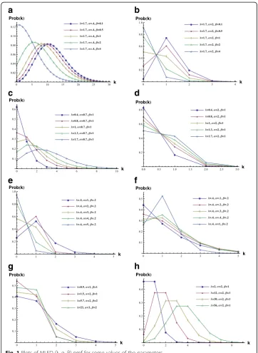
It may be noted that the proportion of zeros given by P(X= 0) = 1/{Γ(β)Eα,β(λ)},
increases with increase inβ(see Fig. 1(b)) when (λ,α) are fixed; increases with decrease in λ (see Fig. 1(c) and (d)) for fixed (α,β); and increases (decreases) withα> (<) 1 (see Fig. 1(e) and (f )) for fixed (λ,β). Whereas when β→0+ the proportion of zeros decreases (see Fig. 1(b)) with the pmf proportional toλk/Γ(αk) ,k= 0, 1, 2,⋯.
Recurrence relation between probabilities
The MLFD (λ,α,β) pmf in (5) has a simple recurrence relation given by
Γ αð kþαþβÞP Xð ¼kþ1Þ ¼λ Γ αð kþβÞP Xð ¼kÞ;k≥1 ð6Þ
withP(X= 0) = 1/{Γ(β)Eα,β(λ)}.
Whenαis a positive integer, (6) can be expressed as (αk+β)αP(X=k+ 1) =λP(X=k). The distribution exhibits long tailedness for 0 <α< 1 as the ratio of successive prob-abilities varies slowly (this corresponds to over-dispersion) as ktends to infinity while forα≥1 this ratio tends to zero faster implying presence of a Poisson-type tail.
The recurrence relation in (6) facilitates easy computation of the probabilities. The computation of the normalizing constant Eα,β(λ) is only required forP(X= 0).
Note that the recurrence relation (or the difference equation) in (6) reduces to that of HP (λ,β) distribution forα= 1 and displaced Poisson distribution whenα= 1 andβis an integer (further discussed in Section 2.5.1).
Computation of the generalized Mittag-Leffler function Eαβ(λ)
For statistical inference and applications it is necessary to compute the generalized Mittag-Leffler functionEα,β(λ), which is the normalizing constant, where
Eα;βð Þ ¼λ X∞
j¼0
λj=Γ αð jþβÞ:
Numerical computation of the generalized Mittag-Leffler function is well-researched. Seybold and Hilfer (2008) gave a numerical algorithm for calculating the generalized Mittag-Leffler function for arbitrary complex argumentzand real parametersαandβbased on a Taylor series, exponentially improved asymptotics and integral representation. If |λ|≤ 1, a simple way to computeEα,β(λ) is to calculate the termsaj=λj/Γ(αj+β) in the infinite
Lee et al., 2001). This avoids the computation of the gamma functionΓ(x). The summation is terminated whenajis very small. The error estimate is given by Theorem 4.1 of Seybold
and Hilfer (2008) which determines the number of termsNsuch that
Eα;βð Þλ ≈ XN
j¼0
λj=Γ αjð þβÞ:
For other values of λ, asymptotic series and integral representation (see equations (2.3), (2.4) and (2.7) of Seybold and Hilfer, 2008) are employed. Error estimates are also
given for these cases. The computation of the Mittag-Leffler function is given by many software packages like Matlab (MLF (alpha, Z, P)) and Mathematica (MittagLefflerE [a, b, z]). (See also Gorenflo et al., 2002.) See also Garrappa (2015) for a recent contribution towards numerical evaluation of Mittag-Leffler function.
Shapes of pmf
The pmf of MLFD (λ,α,β) is plotted for a number of combinations of parameters to study the different shapes of the distribution.
From the plots of the pmf it is seen that the distribution can be unimodal with non-zero mode (see Fig. 1(a)) or it can have nonnon-zero modes at two points (see Fig. 1(h)) or non-increasing with the mode at 0 (see Fig. 1(g)). See Section 4.3 item (i) for further discussion on the modes.
Cumulative distribution function and generating functions
The cumulative distribution function (cdf ) ofX~ MLFD (λ,α,β) is seen to be
P X≤rð Þ ¼1−λrþ1Eα;βþðrþ1Þαð Þλ =Eα;βð Þλ
by using the known relation λrEα;βþrαð Þ ¼λ Eα;βð Þ−λ Xr−1
j¼0
λj=Γ αð jþβÞ (Haubold et
al., 2011).
The pgf is given in terms ofEα,β(λ) as
P sð Þ ¼E s X ¼Eα;βð Þλs =Eα;βð Þλ ;0<λs
The moment generating function (mgf ) and the factorial moment generating func-tion (fmgf ) are obtained from the pgf as
Eα;βðλesÞ=Eα;βð Þλ andEα;βðλð1þsÞÞ=Eα;βð Þλ respectively:
Related distributions and connections with other families of distributions Particular cases of MLFD (λ,α,β)
The MLFD (λ,α,β) includes a number of well-known distributions as particular cases:
(i) Whenα=β= 1, MLFD (λ,α,β) reduces to the Poisson distribution with parameterλ. (ii)Whenα= 0,β(≥0) MLFD (λ,α,β) becomes the geometric distribution with parameterλ
provided 0 <λ< 1. Since forα→0+, lim
α→0þEα;βð Þλ →
X∞
j¼0 λj
Γ βð Þ¼ð1−λ1ÞΓ βð Þ;0<λ<1 (Hanneken et al.,2009).
(iii) Whenα= 1,β(≥0) MLFD (λ,α,β) reduces to the HP (λ,β) distribution (Bardwell and Crow,1964; Johnson et al.,2005, p. 200).
Proof: P Xð ¼kÞ ¼ΓðkþβλÞkE
1;βð Þλ; k¼0;1;2;⋯;λ>0 where E1;βð Þ ¼λ X∞
j¼0
λj=Γ jþβ
ð Þ ¼
X∞
j¼0
λj= ð Þβ jΓ βð Þ
n o
¼ 1
Γ βð Þ X∞
j¼0
1
ð Þj
β
ð Þj
λj j! ¼
φð1;β;λÞ
Γ βð Þ .
PðX ¼kÞ ¼ Γðβ−1Þ ΓðkþβÞ
e−λλkþβ−1
γðβ−1;λÞ; k¼0; 1; 2;⋯;λ>0; β>1;
sinceE1;βð Þ ¼λ λ
1−βeλγ βð −1;λÞ
Γ βð−1Þ (see Simon, 2013), whereγðu;λÞ ¼ Zλ
0
e−yyu−1dyis the
in-complete gamma function.
(iv) Whenα= 1 andβ(=t+ 1) is a positive integer, MLFD (λ,α,β) reduces to the displaced Poisson distribution (see Staff,1964; Johnson et al.,2005, p. 200) with parameterλandt.
In addition, the following new distributions involving hyperbolic and error functions are also seen as particular cases.
(v)Whenα= 2 andβ= 2, MLFD (λ,α,β) reduces to a new discrete distribution with parameterλand pmf
P Xð ¼kÞ ¼ λ kþð1=2Þ Γð2ðkþ1ÞÞ
1 sinhpffiffiffiλ ¼
ffiffiffi λ
p
2kþ1
2kþ1
ð Þ!
1
sinhpffiffiffiλ ; k¼0;1;2;⋯;λ>0;
sinceE2;2ð Þ ¼λ sinh ffiffiffi
λ
p
=pffiffiffiλ(Haubold et al., 2011).
(vi) Whenα= 2 andβ= 1, MLFD (λ,α,β) reduces to a new distribution with parameter λand pmf
P Xð ¼kÞ ¼ λ k Γð2kþ1Þ
1 coshpffiffiffiλ ¼
ffiffiffi λ p 2k 2k ð Þ! 1
coshpffiffiffiλ ;k¼0;1;2;⋯;λ>0
sinceE2;1ð Þ ¼λ cosh ffiffiffi
λ
p
(Haubold et al., 2011).
(vii)Whenα= 1/2 andβ= 1, MLFD (λ,α,β) reduces to a new distribution with parameterλand pmf
P Xð ¼kÞ ¼ exp −λ 2
λk k=2
ð Þ!erfcð Þ−λ ; k¼0;1;2;⋯;λ>0
sinceE1=2;1 ffiffiffiλ
p
¼ expð Þλ erfc−pλffiffiffi (Haubold et al.,2011) whereerfc(λ) is the
complementary error function defined aserfcð Þ ¼λ 1−erfð Þ ¼λ 1−2ffiffiffi π
p
Zλ
0
exp−t2 dt.
Also erfcð Þ ¼λ 2 1ffiffiffiffi 2π p
Z
−∞ −pffiffi2λ
expð−t2=2Þdt 2
4
3
5¼2Φ−pffiffiffi2λ , Φ(.) being the cdf of the
(viii) MLFD (λ,α,β) degenerates with mass only at zero for eitherα→∞orβ→∞or both and also whenλ→0+.
Remark 2. For 0≤α≤1, the MLFD (λ,α,β) can be viewed as a continuous bridge
between the geometric (α= 0) and HP (α= 1) distributions in the range of the param-eter α; in particular, the MLFD (λ,α, 1) can be viewed as acontinuous bridge between the geometric (α= 0) and Poisson (α= 1) distributions in the range of the parameterα, a property also shared by the COM-Poisson distribution.
MLFD as weighted Poisson distribution
The MLFD (λ,α,β) is seen as a weighted Poisson distribution as follows: IfX~ Poisson (λ) having pmf
P Xð ¼kÞ ¼e−λλk=k!; k¼0;1;2;⋯;λ>0;
then for integer α and β it can be shown that weighted distribution with weight function 1/(k+ 1)(α−1)k+β−1 gives the pmf of MLFD (λ,α,β). Since the weight function 1/(k+ 1)(α−1)k+β−1 is monotonically decreasing ink for α,β> 1, MLFD (λ, α,β) is stochastically smaller than the Poisson distribution when α,β> 1. (See Patil et al. 1986; Ross, 1983; Castillo and Pérez-Casany, 2005)
MLFD as member of some families of discrete distributions
i. MLFD (λ,α,β) is a member of the generalized hypergeometric family (Kemp1968a, b). This can be checked by comparing the recurrence relation in Eq. (6) with that of the generalized hypergeometric distributions (see equation (2.63) in page 91 of Johnson et al.,2005).
ii. MLFD (λ,α,β) is a member of the generalized power series distribution (Patil1962, 1964) whenλis the primary parameter.
iii. For fixed values of the parametersαandβ, the MLFD (λ,α,β) is also a member of the exponential family of distributions.
Moments and related results
Denoting E Xð Þ ¼r μ=
r , E(X[r]) =μ[r] and E[{X−E(X)}r] =μr, x[r]=x(x−1)⋯(x−r+ 1) and using the relationE X½ r
¼μ=
r ¼ d
r
dsrP sð Þjs¼1, whereP(s) is the pgf of MLFD (λ,α,β)
mentioned in Section 2.4, and along with a result for the derivative of Eα,β(λ) with respect toλgiven by
d
dλEα;βð Þ ¼λ
Eα;β−1ð Þλ −ðβ−1ÞEα;βð Þλ
αλ ;
we can derive the following formulas:
μ=1¼λddλlogEα;βð Þλ
¼ Eα;β−1ð Þλ
αEα;βð Þλ−
1−β
α, providedα> 0 andβ> 1.
μ=2¼ 1 α2
Eα;β−2ð Þλ
Eα;βð Þλ − 2β−3
α2
Eα;β−1ð Þλ Eα;βð Þλ þ
β−1 α
2
μ2¼α12
Eα;β−2ð Þλ Eα;βð Þλ −
Eα;β−1ð Þλ Eα;βð Þλ
2
þEα;β−1ð Þλ Eα;βð Þλ
) (
, providedα> 0 andβ> 2.
μ2¼λ d dλμ
= 1¼λ
d dλ λ
d
dλlog Eα;βð Þλ
¼λ d
dλlog Eα;βð Þλ
þλ2 d2
dλ2 log Eα;βð Þλ
The above results can alternatively be derived easily by first derivingE(αX+β)[r],r= 1, 2
and then simplifying.
In all the above expressions there is restriction on the values of β. This situation may be overcome by using the following relation repeatedly till the conditions are satisfied:
Eα;βð Þ ¼λ ð1=Γ βð ÞÞ þλEα;αþβð Þλ
(see Erdelyi 1955; Hanneken et al., 2009).
The gamma function for negative argument can be computed using the formula (Fisher and Kilicman, 2012)
Γð Þ ¼−n −Γ−ð−nþ1Þ=n; whenn≠1;2;⋯ 1
ð Þn=
n!fρð Þn−γg;n¼1;2;⋯
whereρð Þ ¼n X n
i¼1
1
i andγ=−Γ
/
(1) is the Euler’s constant.
Recurrence relations of moments
The following recurrence relations hold:
(i) μ=rþ1¼λdλd μ=rþμ=rμ = 1
(ii) μrþ1¼λ d
dλμrþrμr−1μ2
(iii) μ½rþ1 ¼λ
d
dλμ½ r þ μ = 1−r
μ½ r
(iv) EðαðX−1Þ þβÞα¼λþðβ−αÞαP Xð ¼0Þ
The relations (i) to (iii) can be proved by using the general relations for GPSD or by direct manipulation while (iv) follows from the difference equation in (6).
Sinceμ2> 0 andλ≠0,μ2¼λddλμ
=
1>0 impliesddλμ
=
1>0. Henceμ
=
1 is a monotonically
increasing function ofλ.
Alternative formulae for moments
An alternative formula for moments is given by
E Xð þ1Þr¼r!Erþ1
α;βð Þλ =Eα;βð Þλ , whereEα;βρð Þ ¼λ
X∞
k¼0
ρ ð Þk
k!
λk
Γ αð kþβÞis the generalized Mittag-Leffler function (Prabhakar, 1971).
Proof:E Xð þ1Þr¼X
∞
k¼0
kþ1
ð Þrλk
Γ αð kþβÞEα;βð Þλ ¼
r!
Eα;βð Þλ X∞
k¼0 rþ1
ð Þk
k!
λk
Γ αð kþβÞ
¼r!Erþ1α;βð Þλ =Eα;βð Þλ
sincek! (k+ 1)r=r! (r+ 1)k.
Approximation of the mean and variance for large values ofλ
Using the result that for large values of λ, Eα,β(λ)→{λ(1−β)/αexp(λ1/α)}/α (see
follows from either μ=1¼ Eα;β−1ð Þλ αEα;βð Þλ þ
1−β
α or directly from μ=1¼λddλlogEα;βð Þλ
. Then
variance can be obtained by using the relation μ2¼λ d dλμ=1.
In particular for MLFD (λ,α, 1) the approximate mean and variance will be λ1/α/α and λ1/α/α2. These approximations are good whenα∈(0, 2] (see Simon, 2013) and may be useful in a regression formulation where the covariates are linked through the mean and variance.
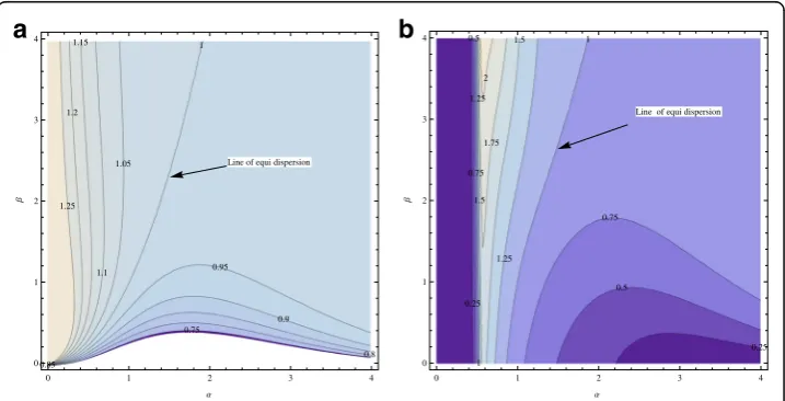
Index of dispersion
The index of dispersion (ID) is given by ID = Variance/Mean. Contour plots of ID for different choices of parameters (α,β) keeping λ= 0.25 andλ= 5 fixed are presented in Fig. 2(a) and (b) respectively to depict the contours of ID. Labels on a given line indi-cate the value of ID on that line. In these figures, the ID of the region on the left (right) of a given line is more (less) than the ID value on that given line.
From Fig. 2 (a) and (b), it is obvious that the MLFD (λ,α,β) is very flexible with respect to the ID and is able to accommodate under-, equi- and over- dispersion in count data. Interestingly, this family includes a non-Poisson distribution with equi-dispersion whenλ is kept fixed. Some such pairs of values for (α,β) can be easily taken from line of equi-dispersion in the contour plots in Fig. 2(a) when λ= 0.25 and from Fig. 2(b) whenλ= 5.
Using results of the Section 2.6.3 for large values of λ it can be stated that the ID of MLFD (λ,α,β) is approximately given by λ1/α/α((1−β) +λ1/α) which reduces to 1/α for MLFD. (λ,α, 1). Thus for largeλMLFD (λ,α, 1) expected to be over (under)- dispersed de-pending onα< (>)1, while MLFD (λ,α,β) will be under-dispersed in the regionα> 1,β< 1.
MLFD (z,α, 1) as a distribution in a queuing system
MLFD (z,α, 1), like the COM-Poisson distribution, can be derived as the probability of the system being in thek-th state for a queuing system with state dependent service rate.
Consider a queuing system with Poisson inter arrival times with parameter λ, first-come- first-served policy, and exponential service times that depend on the system
0.75
0.8 0.85
0.9 0.95 1
1.05
1.1 1.15
1.2
1.25
Line of equi dispersion
0 1 2 3 4
0 1 2 3 4
0.25
0.25 0.5
0.5
0.75
0.75 1
1 1.25 1.25
1.5
1.5 1.75 2
Line of equi dispersion
0 1 2 3 4
0 1 2 3 4
a
b
state (n-th state meansnnumber of units in the system). The mean service time in the
n-th state is μn=μ(nα)[α],n≥1 and μn=μ for α= 0, where, 1/μ is the normal mean
service time for a unit when that unit is the only one in the system and αis the pres-sure coefficient, a constant reflecting the degree to which the service rate of the system is affected by the system. For the sake of completeness, the proof that the probability is the pmf of MLFD (z,α, 1) wherez=λ/μis given as follows:
Following Conway and Maxwell (1962, p. 134–35), the system of differential differ-ence equations are
P0ðtþΔÞ ¼ð1−λΔÞP0ð Þ þt μ1ΔP1ð Þt ð7Þ
and
PnðtþΔÞ ¼ 1−λΔ−ð Þnα ½ αμΔ
Pnð Þ þt λΔPn−1ð Þ þt ððnþ1ÞαÞ½ αμΔPnþ1ð Þt ;n
¼1;2;⋯ ð8Þ
From (7) we get P0(t+Δ)−P0(t) =−λ ΔP0(t) +μ α! ΔP1(t) sinceμ1=μ(α)α=μα!. This
implies, lim Δ→0
P0ðtþΔÞ−P0ð Þt
Δ ¼−λP0ð Þ þt μα!P1ð Þt
orP=0ð Þ ¼t −λP0ð Þ þt μα!P1ð Þt .
Assuming a steady state (i.e. P=nð Þ ¼t 0 for alln), we getP1(t) =zP0(t)/α! whereλ/μ=z. Similarly, from (8), we get
lim Δ→0
PnðtþΔÞ−Pnð Þt
Δ ¼− λþð Þnα ½ αμ
Pnð Þ þt λPn−1ð Þ þt ððnþ1ÞαÞ½ αμPnþ1ð Þt .
It follows that
P=nð Þ ¼t − λþð Þnα ½ μα
Pnð Þ þt μz Pn−1ð Þ þt ððnþ1ÞαÞ½ μα Pnþ1ð Þ ¼t 0
becauseP=nð Þ ¼t 0 for allnandλ/μ=z.
This implies that (z+ (nα)[α])Pn(t) =z Pn−1(t) + ((n+ 1)α)[α]Pn+ 1(t) sinceμ≠0.
Puttingn= 1 we get
(z+α!)P1(t) =zP0(t) + (2α)[α]P2(t),
P2(t) = {z2/(2α) ! }P0(t). Sinceα! (2α)[α]= (2α) ! Similarly, forn= 2 we get
zþð Þ2α ½ α
P2ð Þ ¼t zP1ð Þ þt ð Þ3α ½ αP3ð Þt
P2(t) = {z3/(3α) ! }P0(t), since (3α! )(3α)[α]= (3α) !
In general,Pn(t) = {zn/(nα) ! }P0(t),
whereP0ð Þ ¼t 1= X∞
n¼0
zn=ð Þ!nα
f g. This is the pmf of MLFD (z,α, 1).
In the case whenαis not an integer one can useα! =Γ(α+ 1).
Reliability, stochastic ordering and log concavity
reliability properties of the proposed discrete distribution. Stochastic ordering is a closely related important area that has found applications in many diverse areas such as economics, reliability, survival analysis, insurance, finance, actuarial and manage-ment sciences (see Shaked and Shanthikumar, 2007). In this section we study the reli-ability properties and stochastic ordering of the MLFD (λ,α,β) distribution.
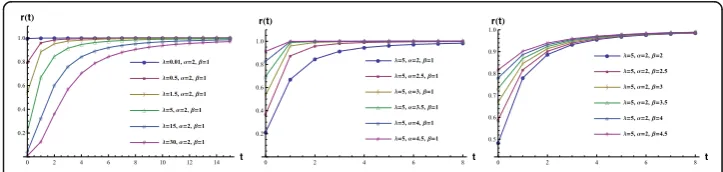
Survival and failure rate function
The survival and failure rate function for MLFD (λ,α,β) are respectively given by
S tð Þ ¼P Xð >tÞ ¼λtþ1 Eα;βþðtþ1Þαð Þλ =Eα;βð Þλ and r tð Þ ¼P Xð ¼tÞ=P Xð ≥tÞ ¼1=Γ αð tþβÞEα;βþtαð Þλ :
This distribution has non decreasing failure rate function which we have shown later in section 4.3. The failure rate function r(t) is plotted in Fig. 3 for some choices of parameters to see how it behaves with changing parameter values. The values of r(t) tend to increase withαorβbut decrease with increase inλwhen other two parameters are kept fixed.
Stochastic ordering with HP
The following result stochastically compares the MLFD (λ,α,β) with the HP (λ,β) by using the likelihood ratio order.
Definitions: Let X andY be two discrete random variables with pmfsf(x) and g(x). Then X is said to be smaller than Yin the likelihood ratio order denoted byX≤lrYif g(x)/f(x) increases inx over the union of the supports ofX andY; Xis smaller than Y
in the hazard rate orderX≤hrYifrX(t)≥rY(t) for allt;X is smaller thanYin the mean
residual life orderX≤MRLYifμX(t)≤μY(t) for allt, whererX(.) andμX(.) are respectively
the hazard rate and mean residual life (MRL) functions ofX.
Theorem 1. For α> 1, X~MLFD (λ,α,β) is smaller than Y~ HP (λ,β)distribution in the likelihood ratio order i.e. X≤lrY, while for 0 <α< 1, HP (λ,β) is greater than MLFD(λ,α,β)distribution in the likelihood ratio orderi.e.Y≤lrX.
Proof: IfX~ MLFD (λ,α,β) andY~ HP (λ,β) then
P Yð ¼nÞ P Xð ¼nÞ¼
ΓðnαþβÞ ΓðnþβÞ
E1;βð Þλ Eα;βð Þλ
Forα> 1 this ratio is clearly increasing inn(see Shaked and Shanthikumar, 2007 and Gupta et al., 2014). HenceX≤lrYis proved. While for 0 <α< 1, the ratio is decreasing
innwhich proves thatY≤lrX.
Corollary 1. For α> 1, X~ MLFD (λ,α,β) is smaller than Y~ HP (λ,β) distribution in the MRL life order that isX≤MRLY.
Proof.The result follows sinceX≤lrY⇒X≤hrY⇒X≤MRLY. (see Gupta et al., 2014).
Log-concavity
The log-concavity of any probability distribution has important implications on its reli-ability function, failure rate function, tail probabilities and moments. The MLFD (λ,α,β) has a log-concave pmf since for this distribution (Gupta et al., 1997)
Δη
ð Þ ¼
t
P tðP tð Þþ1Þ−
P tP tððþþ21ÞÞ¼
λ
Γ αð tþβΓ αÞðΓ αðtþtαþþ2βαÞþΓ αðβÞ−tþfΓ α2ðαþtþβÞαþβÞg2> 0. The following results are direct consequence of log-concavity (Mark, 1996):i. MLFD (λ,α,β) is a strongly unimodal distribution due to the log-concavity of its pmf (see Steutel1985).
➢MLFD (λ,α,β) has a unique modeat X=k if
Γ αkð þβÞ=Γ αkð −αþβÞ<λ<Γ αkð þαþβÞ=Γ αkð þβÞ
Proof: This follows easily from the probability recurrence relation given in (5).
➢MLFD (λ,α,β) has a non increasing pmf with a unique mode atX= 0 ifλ <Γ(α+β)/Γ(β) (See the pmf plots in Fig.1(g) for some choices of (λ,α,β) satisfying the condition.)
➢MLFD (λ,α,β) has two modesat X=kandX=k+ 1 if
λ¼Γ αkð þαþβÞ=Γ αkð þβÞ
(See the pmf plot in Fig.1(h) for some (λ,α,β) satisfying the condition.)
ii. MLFD (λ,α,β) has non decreasing failure rate function. iii. MLFD (λ,α,β) has at most an exponential tail.
iv. MLFD (λ,α,β) remains log-concave if truncated.
v. P XðP Xð¼¼iþiÞkÞ
≥
P XðP Xð¼¼jþjÞkÞfor
i
<
j
.Data Fitting
Parameter estimation
Suppose that we have a sample of size n from MLFD (λ,α,β) reported as grouped frequencies in k classes, like (X,f) = {(x1,f1), (x2,f2,), . . . , (xk,fk)}, where fi is the
frequency of i-th observed value xi and n=∑fi is the sample size. Then the
log-likelihood function is given by
logL xð 1;x2;⋯;xkjλ;α;βÞ ¼ Xk
i¼1 fixi
!
logλ−X
k
i¼1
filogΓ αð xiþβÞ−nlogEα;βð Þλ .
Numerical examples
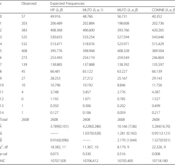
Here we have considered two frequency data sets. The first data set in Table 1 is about trips made by Dutch households owning at least one car during a particular survey week in 1989 (van Ophem, 2000). This data is slightly over-dispersed with Mean = 3.038, Variance = 3.410 and index of dispersion (ID) = 1.123. The second data set in Table 2 is the frequency distribution of theα- particles emitted by a radioactive substance in 2608 periods, each of 7.5 sec (Rutherford and Geiger, 1910). This data is slightly under-dispersed with Mean = 3.872, Variance = 3.695 and index of ID = 0.9543
The MLFD (λ,α,β) model is a generalization/extension of the HP (λ,β) and MLFD (λ,α, 1). Therefore the MLFD (λ,α,β) model has been fitted and compared with the HP (λ,β), MLFD (λ,α, 1) to ascertain the benefits accrued through the proposed generalization. In addition, we have also considered a recently introduced three-param-eter distribution namely the COM-Poisson type negative binomial [COMNB (λ,α, β)] distribution having pmf P(X=k) = (λ)kαk/{(k!)βSβ,λ(α)}, k= 0, 1, 2,⋯ where
Sβ,λ(α) is the normalizing constant (Chakraborty and Ong, 2016) for comparative data fitting. The performances of various distributions are compared using the AIC
Table 1Observed and expected frequencies of trips made by Dutch households owning at least
one car during a particular survey week in 1989(van Ophem, 2000)
x Observed Expected Frequencies
HP (λ,β) MLFD (λ,α, 1) MLFD (λ,α,β) COMNB (λ,α,β)
0 75 93.208 99.150 74.175 89.965
1 312 269.133 273.608 308.769 284.076
2 384 403.029 399.3458 420.586 411.107
3 421 407.420 399.724 389.683 397.963
4 307 310.848 305.795 286.233 296.794
5 183 190.456 189.821 178.113 183.213
6 77 97.491 99.311 97.428 97.687
7 47 42.853 44.958 47.962 46.258
8 15 16.504 17.9533 21.598 19.836
9 9 5.656 6.4181 9.003 7.813
10 5 1.746 2.078 3.506 2.858
11 0 0.490 0.615 1.285 0.979
12 0 0.126 0.166 0.445 0.316
13 1 0.030 0.042 0.147 0.097
14 2 0.007 0.010 0.046 0.028
15 0 0.001 0.002 0.014 0.008
16 0 0.000 0.000 0.004 0.002
17 1 0.000 0.000 0.002 0.001
Total 1839 1839 1839 1839 1839
^
λ 3.110 (0.121) 2.697 (0.182) 1.000 (0.130) 3.288 (4.25)
^
α —— 0.943 (0.032) 0.576 (0.063) 0.960 (1.22)
^
β 1.080(0.121) —— 0.183 (0.058) 1.509 (0.40)
χ2, df 37.034, 7 32.564, 8 17.716, 8 20.676, 8
p-val <0.01 <0.01 0.023 <0.01
(Akaike Information Criterion) defined as AIC =−2 log L+ 2k, where k is the number of parameter(s) and log L is the maximum of log-likelihood for a given data set (Burnham and Anderson, 2004). We also provide chi-square goodness of fit statistics with p-values. In Tables 1 and 2 the degrees of freedoms for χ2 are given alongside its value and the standard errors for parameter estimates are given within parentheses.
From Table 1 it can be seen that the MLFD (λ,α,β) gives the best fit since it has the lowest χ2value and is also the first choice in model selection with lowest AIC value. Moreover MLFD (λ,α,β) is the only distribution with good fit at 1% since itsp-value is more than 0.01 while for the rest thep-values are less than 0.01.
From Table 2 considering the χ2values together with p-values it can be seen that all the distributions except the COMNB (λ,α,β) give adequate fits. But among them the MLFD (λ,α,β) gives the best fit since it has the lowest value of χ2 with the highestp-value. It is also the selected model because it has the lowest AIC value.
Conclusion
A new generalization of the HP distribution which is a continuous bridge between the geometric and HP is derived using the generalized Mittag-Leffler function. Some known and new distributions are seen as particular cases of this distribution. This new
Table 2Frequency distribution of theα- particles emitted by a radioactive substance in 2608
periods (Rutherford and Geiger, 1910)
x Observed Expected Frequencies
HP (λ,β) MLFD (λ,α, 1) MLFD (λ,α,β) COMNB (λ,α,β)
0 57 49.916 48.766 56.731 40.352
1 203 206.489 202.884 198.608 202.736
2 383 408.368 406.600 393.766 420.265
3 525 530.655 533.254 527.594 543.646
4 532 513.471 518.076 523.971 515.429
5 408 395.776 398.948 408.328 389.504
6 273 253.493 254.119 259.549 246.804
7 139 138.885 137.888 138.392 135.597
8 45 66.481 65.122 63.227 66.139
9 27 28.253 27.212 25.167 29.143
10 10 10.796 10.192 8.846 11.756
11 4 3.748 3.457 2.776 4.387
12 0 1.192 1.071 0.785 1.527
13 1 0.350 0.306 0.202 0.499
14 1 0.127 0.106 0.059 0.217
Total 2608 2608 2608 2608 2608
^
λ 3.789(0.101) 4.228(0.286) 10.166 (7.06) 5.284(16.70)
^
α —— 1.037(0.028) 1.281 (0.182) 0.951(3.121)
^
β 0.916(0.096) —— 2.170 (1.044) 1.527(0.921)
χ2
, df 18.382, 11 11.367, 10 8.179, 9 22.326, 9
p-val 0.073 0.330 0.516 0.008
generalization belongs to the generalized power series, generalized hypergeometric fam-ilies and also arises as weighted Poisson distributions. Like the HP, COM-Poisson and generalized Poisson distributions, this distribution is also able to cater for under-, equi-and over- dispersion. Although the new generalization of the HP distribution has an extra parameter, it is computationally not more complicated than the HP since it retains the two-term probability recurrence formula and the normalizing constant, in terms of the generalized Mittag-Leffler function, is readily computed. It has many inter-esting probabilistic and reliability properties and is found to be a better empirical model than the HP distribution.
Acknowledgements
The first author wishes to acknowledge the hospitality of Institute of Mathematical Sciences, University of Malaya during his visit to the institute in the summer of 2014. S.H. Ong wishes to acknowledge support in parts from Ministry of Education FRGS grant FP045-2015A and University of Malaya’s UMRGS grant RP009A-13AFR. The authors also wish to acknowledge the significant comments and suggestions of the Associate Editor and reviewers in earlier versions of the paper which have helped to improve the presentation tremendously.
Authors’contributions
Both authors read and approved the final manuscript.
Competing interests
The authors declare that they have no competing interests.
Publisher’s Note
Springer Nature remains neutral with regard to jurisdictional claims in published maps and institutional affiliations.
Author details
1Department of Statistics, Dibrugarh University, Dibrugarh 786004, Assam, India.2Institute of Mathematical Sciences,
University of Malaya, 50603 Kuala Lumpur, Malaysia.
Received: 18 February 2016 Accepted: 29 May 2017
References
Ahmad, M.: A short note on Conway-Maxwell-hyper Poisson distribution. Pak J Stat23, 135–137 (2007) Antic, G., Stadlober, E., Grzybek, P., Kelih, E.: Word length and frequency distributions in different text genres. In:
Spiliopoulou, M., Kruse, R., Nürnberger, A., Borgelt, C., Gaul, W. (eds.) From Data and Information Analysis to Knowledge Engineering, pp. 310–317. Springer, Heidelberg (2006)
Bardwell, G.E., Crow, E.L.: A two parameter family of hyper-Poisson distributions. J Am Stat Assoc59, 133–141 (1964) Best, K.: Kommentierte Bibliographie zum Göttinger Projekt. In: Best, K.-H. (ed.) Häufigkeitsverteilungen in Texten, pp.
248–310. Pest & Gutschmidt, Göttingen (2001)
Burnham, K.P., Anderson, D.R.: Multimodel Inference, Understanding AIC and BIC in model selection. Sociological Methods and Research33, 261–304 (2004)
Cameron, A.C., Johansson, P.: Count Data Regression Using series expansions: with applications. J Appl Econ12(3), 203–223 (1997)
Castillo, J.D., Pérez-Casany, M.: Over-dispersed and under-dispersed Poisson generalizations. Journal of Statistical Planning and Inference134, 486–500 (2005)
Chakraborty, S., Ong, S.H.: A COM-Poisson-type generalization of the negative binomial distribution. Communications in Statistics -Theory and Methods45(14), 4117–4135 (2016)
Consul, P.C.: Generalized Poisson distributions: properties and applications. Marcel Dekker Inc, New York/Basel (1989) Conway, R.W., Maxwell, W.L.: A queuing model with state dependent service rates. J Ind Eng12, 132–136 (1962) Crow, E.L., Bardwell, G.E.: Estimation of the parameters of the hyper-Poisson distributions. In: Patil, G.P. (ed.) Classical and
Contagious Discrete Distributions, pp. 127–140. Pergamon, Oxford (1965)
Devroye, L.: A note on Linnik’s distribution. Statistics and Probability Letters9, 305–306 (1990)
Efron, B.: Double Exponential-Families and their use in Generalized Linear-Regression. J Am Stat Assoc81(395), 709–721 (1986) Erdelyi, A.: Higher transcendental functions, vol. 3. McGraw-Hill, New York (1955)
Fisher, B., Kilicman, A.: Some results on the gamma function for negative integers. Appl Math Inf Sci6(2), 173–176 (2012) Garrappa, R.: Numerical evaluation of two and three parameter Mittag-Leffler functions. Siam J Numer
Anal53(3), 1350–1369 (2015)
Gerhold, S.: Asymptotics for a variant of the Mittag-Leffler function. Integral Transforms and Special functions23(6), 397–403 (2012)
Gorenflo, R., Joulia, L., Luchko, Y.: Computation of the Mittag-Leffler function Eα,β(z) and its derivatives. Fractional Calculus & Applied Analysis5(4), 491–518 (2002)
Gupta, R.C., Sim, S.Z., Ong, S.H.: Analysis of discrete data by Conway-Maxwell Poisson distribution. AStA Advances in Data Analysis98, 327–343 (2014)
Hanneken, J.W., Achar, B.N.N., Puzio, R., Vaught, D.M.: Properties of the Mittag–Leffler function for negative alpha. Phys Scr. T136, 014037, 1–5 (2009). doi:10.1088/0031-8949/2009/T136/014037
Haubold, H.J., Mathai, A.M., Saxena, R.K.: Mittag-Leffler functions and their applications. J Applied Math, Article ID 298628, p. 51 (2011). doi:10.1155/2011/298628
Jayakumar, K.: On Mittag-Leffler process. Math Comput Model37, 1427–1434 (2003)
Jayakumar, K., Pillai, R.N.: The first order autoregressive Mittag-Leffler process. J Appl Probab30, 462–466 (1993) Johnson, N.L., Kemp, A.W., Kotz, S.: Univariate Discrete Distributions. Wiley, New York (2005)
Jose, K.K., Abraham, B.: A count data model based on Mittag-Leffler inter arrival times. Statistica71(4), 501–514 (2011) Jose, K.K., Pillai, R.N.: In: Yagen Thomas, P. (ed.) Generalized autoregressive time series models in Mittag-Leffler variables.
Recent Advances in Statistics, pp. 96–103. (1986)
Jose, K.K., Uma, P., Seethalekshmi, V., Haubold, H.J.: Generalized Mittag-Leffler processes for applications in astrophysics and time series modelling. In: Haubold, H.J., Mathai, A.M. (eds.) Proceedings of the third UN/ESA/NASA workshop on the International Heliophysical Year 2007 and Basic sciences, Astrophysics and Space Science Proceedings, pp. 79–92. (2010). doi:10.1007/978-3-642-03325-4_9
Kemp, A.W.: Studies in Univariate discrete distribution theory based on the generalized hypergeometric function and associated differential equations. PhD Thesis. The Queen’s University of Belfast, Belfast (1968a)
Kemp, A.W.: A wide class of discrete distributions and the associated differential equations. Sankhya, Series A30, 401–410 (1968b)
Kemp, C.D.: q-analogues of the hyper-Poisson distribution. Journal of Statistical Planning and Inference101, 179–183 (2002) Khazraee, S.H., Sáez-Castillo, A.J., Geedipally, S.R.: Lord D: Application of the hyper-Poisson generalized linear model for
analyzing motor vehicle crashes. Risk Anal35(5), 919–930 (2015)
Kumar, C.S., Nair, B.U.: A modified version of hyper-Poisson distribution and its applications. J Stat Appl6, 23–34 (2011) Kumar, C.S., Nair, B.U.: An alternative hyper-Poisson distribution. Statistica3, 357–369 (2012)
Kumar, C.S., Nair, B.U.: Modified alternative hyper -Poisson distribution. In: Kumar, C.S., Chacko, M., Sathar, E.I.A. (eds.) Collection of recent statistical methods and applications, Department of Statistics, pp. 97–109. University of Kerala publication, Trivandrum (2013)
Kumar, C.S., Nair, B.U.: On a class of hyper-Poisson and alternative hyper-Poisson distributions. OPSEARCH (Operational Research Society of India)52(1), 86–100 (2015). doi:10.1007/s12597-013-0169-7
Lee, P.A., Ong, S.H., Srivastava, H.M.: Some integrals of the products of Laguerre polynomials. Internat J Comput Math78, 303–321 (2001)
Lin, G.D.: On Mittag-Leffler distribution. Journal of Statistical Planning and Inference74, 1–9 (1998)
Mark, Y.A.: Log-concave probability distributions: Theory and statistical testing. Working paper, Published by Center for Labour Market and Social Research, University of Aarhus and the Aarhus School of Business, Working
Paper 96–01, (1996)
Mittag-Leffler, G.: Sur la nouvelle fonction Eα(x). Comptes Rendus Acad Sci Paris137, 554–558 (1903) Mittag-Leffler, G.: Sur la représentation analytique d’une branche uniforme d’une fonction monogene. Acta
Math29, 101–181 (1905)
Patil, G.P.: Estimation by two moments method for generalized power series distribution and certain applications. Sankhya, B24(3&4), 201–214 (1962)
Patil, G.P.: In: Rao, C.R. (ed.) Estimation for the generalized power series distribution with two parameters and its application to binomial distribution. Contributions to Statistics, pp. 335–344. Calcutta: Statistical Publishing Society; Oxford, Pergamon (1964)
Patil, G.P., Rao, C.R., Ratnaparkhi, M.V.: On discrete weighted distributions and their use in model for observed data. Communications in Statistics-Theory and Methods15(3), 907–918 (1986)
Pillai, R.N.: On Mittag-Leffler functions and related distributions. Ann Inst Statist Math42, 157–161 (1990) Pillai, R.N., Jayakumar, K.: Discrete Mittag-Leffler distributions. Statistics & Probability Letters23, 271–274 (1995) Prabhakar, T.R.: A singular integral equation with a generalized Mittag-Leffler function in the Kernel. Yokohama
Math J19, 7–15 (1971)
Roohi, A., Ahmad, M.: Estimation of the parameter of hyper-Poisson distribution using negative moments. Pak J Stat19, 99–105 (2003a)
Roohi, A., Ahmad, M.: Inverse ascending factorial moments of the hyper-Poisson probability distribution. Pak J Stat19, 273–280 (2003b)
Ross, S.M.: Stochastic Processes. Wiley, New York (1983)
Rutherford, E., Geiger, H.: The probability variations in the distribution ofα- particles. Philos Mag20, 698–704 (1910) Sáez-Castillo, A.J., Conde-Sánchez, A.: A hyper-Poisson regression model for over-dispersed and under-dispersed count
data. Computational Statistics and Data Analysis61, 148–157 (2013)
Seybold, H., Hilfer, R.: Numerical algorithm for calculating the generalized Mittag -Leffler function. SIAM J Numer Anal47(1), 69–88 (2008)
Shaked, M., Shanthikumar, J.G.: Stochastic Orders. Springer Verlag (2007)
Shmueli, G., Minka, T.P., Kadane, J.B., Borle, S., Boatwright, S.: A useful distribution for fitting discrete data-revival of the Conway-Maxwell Poisson distribution. Appl Stat54, 127–142 (2005)
Simon, T.: Mittag - Leffler functions and complete monotonicity. arXiv: 1312. 4513v [math.CA] (2013) Staff, P.J.: The displaced Poisson distribution. Australian Journal of Statistics6, 12–20 (1964)
Staff, P.J.: The displaced Poisson distribution. Region B. Journal of American Statistical Association62(318), 643–654 (1967) Steutel, F.W.: In: Kotz, S., Johnson, N.L., Read, C.B. (eds.) Log-concave and log-convex distributions. Volume 5,
Encyclopedia of Statistical Sciences. (1985)