R E S E A R C H
Open Access
A robust anisotropic diffusion filter with
low arithmetic complexity for images
Resmi R. Nair
1, Ebenezer David
2*and Sivakumar Rajagopal
1Abstract
Image smoothing with edge preservation in the presence of outliers is a challenge in image processing. Anisotropic diffusion smoothing is a well-established paradigm in digital image smoothing with edge preservation. Anisotropic diffusion smoothing filters are not robust to impulse noise. They employ two or more stages for robustness in the presence of outliers, and, therefore, they demand significantly increased arithmetic operations for robustness; consequently, they are not power efficient. This paper introduces a low arithmetic complexity image smoothing model and proposes an intrinsically robust and power efficient algorithm for anisotropic diffusion smoothing of images. The algorithm outperforms the foundational robust smoothing algorithms in terms of the standard performance metrics and visual quality.
Keywords:Anisotropic filters, Computational complexity, Image denoising, Nonlinear filters, Robustness
1 Introduction
Image smoothing is an essential operation in digital image processing. One well-established approach to
image smoothing is scale-space filtering [1]. The
basic scale-space filter is an isotropic diffusion smoothing filter which produces image smoothing with poor edge retention. Perona-Mailk (PM) intro-duced an edge-preserving anisotropic diffusion filter
[2] which also formed the basis for subsequent
de-velopments in anisotropic diffusion smoothing. How-ever, filters based on anisotropic diffusion failed to perform well in the presence of impulse noise. Black et al. [3] developed a statistical interpretation of an-isotropic diffusion from the view point of robust sta-tistics and proposed a diffusion coefficient based on
Tukey’s biweight robust error norm. Ling et al. [4]
proposed a two-stage anisotropic median filtering in which the first stage is anisotropic diffusion; the dif-fusion coefficient is based on Tukey’s biweight ro-bust error norm proposed by Black et al., and the second stage is median filtering of the diffused
image. Ham et al. [5] introduced an adaptive robust
scale-space filter in which the robustness is provided
by the incorporation of a normalization term.
Subse-quent developments [6–13] have followed these
foundational models [2–5].
Wu et al. [6] proposed a two-stage diffusion scheme for random valued impulse noise in which the ENI (edge pixels, noisy pixels, and image pixels) concept is employed in the first stage for the identification of noisy pixels. In the anisotropic diffusion stage, two diffusion functions, namely, controlling speed function and controlling fidelity function are employed for robustness. Wang et al. [7] in-troduced an adaptive switching anisotropic diffusion filter which operates in two modes. In one mode, the filter acts as a direction weighted median filter for impulse noise corrupted pixels, and in the other mode, the filter acts as an adaptive anisotropic diffusion filter for Gaussian noise-corrupted pixels. The filter selects the mode in ac-cordance with a local difference factor of the pixel. Xia et al. [8] proposed a two-stage diffusion filter, which employs a switching function in the diffusion algorithm. The filter
is designed to handle both salt and pepper
noise-corrupted and random-valued impulse
noise-corrupted images. In the first stage, noise detectors are employed to determine the noisy pixels. The value of the switch function in the diffusion algorithm depends on the noise detector output; therefore, the noisy pixels are replaced in the diffusion stage and the uncorrupted pixels are left unchanged. In the second stage, anisotropic * Correspondence:[email protected]
2Department of Electronics and Communication Engineering, Anna
University, Chennai, Tamil Nadu 600025, India
Full list of author information is available at the end of the article
diffusion is carried out at two levels of filtering, namely, coarse filtering and fine filtering for the ef-fective removal of impulse noise. Khan et al. [9]
pro-posed a two-stage robust adaptive anisotropic
diffusion filter. In the preprocessing stage, noisy pixels are identified and are replaced by the median value of the local neighborhood. In the second stage, an adap-tive anisotropic diffusion is carried out. Haiying et al. [10] proposed a two-stage diffusion tensor-based ro-bust diffusion filter. A clean pixel excluder is pro-posed to identify the noisy pixels in the first stage; in the second stage, an adaptive diffusion is carried out in accordance with the diffusion tensor to replace the noisy pixels. Sung et al. [11] proposed a single-pass dictionary-based anisotropic diffusion in which an off-line dictionary and an onoff-line dictionary are employed. In the offline dictionary, diffusivity values and diffusion path kernels for different image patches are stored. A single-pass adaptive anisotropic diffusion is carried out in the online dictionary processing by choosing appropriate diffusivity values and diffusion path-based kernels from the offline dictionary for each image patch. Veerakumar et al. [12] introduced a two-stage adaptive anisotropic diffu-sion filter in which noisy pixel determination is the first stage and an adaptive anisotropic diffusion is the second stage. In the noisy pixel determination stage, each image pixel is compared against the maximum and the mini-mum pixel gray-level values for the determination of salt and pepper noise; a rank-ordered logarithmic difference approach is proposed for the identification of the pixels corrupted by the random-valued impulse noise. In the dif-fusion stage, an adaptive anisotropic difdif-fusion is carried out for the replacement of noisy pixels in accordance with the local neighborhood characteristics.
Existing robust diffusion smoothing filters [4–13] em-ploy a variety of additional nonlinear techniques for im-proving the performance in the presence of outliers. They are generally complex in terms of hardware (adders and multipliers) and are not power efficient. This paper pro-poses a simple first-order anisotropic diffusion model which exhibits a performance superior to the standard
second-order parabolic partial differential equation
(PDE)-based diffusion models. The proposed model is in-trinsically robust, simple in hardware complexity, and power efficient and outperforms the foundational models in terms of performance metrics and visual quality.
The first-order robust diffusion smoothing filter which is intrinsically robust to impulse noise is derived in Sec-tion2based on Albert Einstein’s stochastic argument for
Brownian motion. Section 3 describes the performance
of the proposed filter in detail in comparison with three foundational diffusion smoothing filters [2,4,5] and one extended model [12]. Section 4 concludes by highlight-ing the significance of the proposed filter in the context
of low-power digital signal processing (DSP) and embed-ded environments.
2 The proposed methodology
The methodology is based on the concept that the immediate future value of the intensity of a candi-date pixel can be predicted in terms of the estimate of the increment or decrement of the pixel intensity in terms of the directional derivatives with respect to neighborhood pixels inside an open subset. The open subset includes four neighborhood pixels along the north, south, east, and west directions with re-spect to the center pixel of a 3 × 3 window. The pre-diction equation is a novel mathematical model
developed from Einstein’s stochastic argument for
Brownian motion. The mathematical model involves
a candidate pixel, four neighborhood pixels, a
weighting function, and a control parameter. The mathematical model is translated to an algorithm. For numerical computation of the algorithm, direc-tional derivatives along north, south, east, and west directions of the candidate pixel are calculated; a median estimate of the directional derivatives is ob-tained. The candidate pixel intensity value is updated by adding a value proportional to the median esti-mate of the directional derivatives. This process is repeated for all the pixels in the image. The whole procedure is iterated n times until specified signal to noise ratio performance is achieved. Different test images corrupted with various noise types at differ-ent noise intensities are selected for testing the
algo-rithm. Simulation is carried out on MATLAB
R2014a installed in a system powered by 567u7 Intel (R) core (TM) i5-5200 U CPU @ 2.20 GHz, 64-bit Operating System with 4 GB RAM. The performance of the algorithm is validated in terms of visual re-sults and the performance metrics peak signal to noise ratio (PSNR), structural similarity index metric (SSIM), and edge preservation index (EPI).
2.1 A first-order robust diffusion smoothing model based on Einstein’s stochastic argument for Brownian motion Let I(x,t) be a space-time continuous function at pos-ition xand timet. Following Albert Einstein’s stochastic
argument for Brownian motion of suspended particles in a fluid medium [14], one can write
I xð ;tþτÞ ¼I xð Þ þ;t τð∂I=∂tÞ ð1Þ
I xð Þ þ;t τð∂I=∂tÞ ¼I xð Þ;t
Z þ∞
−∞ ∅ð Þε dε
þð∂I=∂xÞ
Z þ∞
−∞ ε∅ð Þεdε
þ ∂2
I=∂x2
Z þ∞
−∞ ε
2=2
∅ð Þεdε
ð2Þ In (2), I(x,t) and I(x,t+τ) represent the number of Brownian particles per unit volume at time t and t+τ respectively, t+τis the next time instant, ∅(ε) =∅(−ε), R∞
−∞∅ðεÞdε = 1, ε and x are the spatial variables, and ∅(ε) is the probability density distribution function. SinceR−∞∞ ∅ðεÞdε= 1 and∅(ε) =∅(−ε), a simple manipu-lation of (2) eliminates the first term on the left hand side (LHS) and the first and second terms on the RHS of (2). Therefore, (2) can be written as.
∂I=∂t¼ð1=τÞ∂2I=∂x2 Zþ∞
−∞ ε
2=2
∅ð Þεdε
ð3Þ By applying (1) to the LHS of (3)
I xð ;tþτÞ ¼I xð Þ þ;t ð1=τÞ
Z þ∞
−∞ ∂
2
I=∂x2
ε2=2
∅ð Þεdε
ð4Þ Rearranging (4),
I xð ;tþτÞ ¼I xð Þ þ;t ð1=τÞ Z þ∞
−∞ ε
2=2
∅ð Þεdε
∂2I=∂x2
ð5Þ
Let the second term on the RHS of (5) be
inter-preted as a statistical expectation of the directional derivatives ∂I/∂Ex, ∂I/∂Wx resulting from (∂/∂x). (∂I/ ∂x) = (∂2I/∂x2), where I = I(x,t) is the number
dens-ity, E and W are the east and west directions
re-spectively, the dot symbol represents the divergence, and the time t is a parameter. Let (1/τ)∫(ε2/2) ∅(ε)dε be defined as spreading function D(x). Equa-tion (5) says that the function D(x) diffuses the con-centrated mass I(x,t) throughout the length x from x
= x0 to x = xL (x0 and xL are boundaries) with
Gaussian probability density distribution at equilib-rium. In the context of DSP, let this be interpreted as system response to white noise excitation whose autocorrelation is a concentrated impulse [15]. Func-tion D(x) becomes the convolution kernel. Extending (5) to two dimensions
I xð;y;tþτÞ ¼I xð ;y;tÞ þD xð;yÞ∂2I=∂x2þ∂2I=∂y2 ð6Þ
Expression (6) in terms of the inner product becomes
I xð ;y;tþτÞ ¼I xð ;y;tÞ þð∇:D xð ;yÞ∇IÞ; ð7Þ where ∇is the “del” operator and the second term on the RHS of (7) is the divergence of the gradient ofI(x,y,t). Assuming that an image is a volume with one dimension vanishingly small and invoking the divergence theorem
I xð;y;tþτÞ ¼I xð;y;tÞ þ½DN∇NIþDS∇SIþDE∇EIþDW∇WI;
ð8Þ where ∇NI, ∇SI, ∇EI, and ∇WI represent the direc-tional derivatives along north, south, east, and west
di-rections, and DN, DS, DE, and DW are diffusion
functions. Equation (8) describes a spatio-temporal
spreading of the number density I(x,y,t) in which the current value of the number density is updated by a statistical estimate of flux density which tends to reach an equilibrium state such that I(x,y,p+ 1) =
I(x,y,p) after some t = p+ 1 when the probability density distribution of the process settles to Gaussian [16]. Equations (4)–(8) are based on the continuum hypothesis; for sampled time and space variables, the last equation becomes
I uð Δx;vΔy;ðnþ1ÞΔtÞ ¼I uð Δx;vΔy;nΔtÞ
þΔt=ð ÞΔx2:½DN∇NIþDS∇SIþDE∇EIþDW∇WI;
ð9Þ whereΔtis the time sampling interval;ΔxandΔyare the space sampling intervals;u,v, andnare integers including zero; Δx=Δy; and I in the second term on the RHS is
I(uΔx,vΔy,nΔt). If the integersuandvtake a value equal to zero, the corresponding image is the initial or the original image. It becomes an initial value problem which is a necessary condition for a causal Markov process. Consistent with (5), the diffusion of I(uΔx,vΔy,nΔt) is interpreted as the accumulation of the expectation of the directional derivatives with respect to iteration
number n, starting with an initial number density as
a delta function at n = 0. At equilibrium, I(uΔx,
vΔy, (m+ 1)Δt) =I(uΔx,vΔy,mΔt) for some n=m, and is a Gaussian distributed function. Since mean is the posterior estimate in the least square sense for Gaussian distribution [16], (9) can be written as
I uð Δx;vΔy;ðnþ1ÞΔtÞ ¼I uð Δx;vΔy;nΔtÞ
þΔt=ð ÞΔx2:ð Þ4 ½ð1=4ÞðDN∇NIþDS∇SIþDE∇EIþDW∇WIÞ
I uð Δx;vΔy;ðnþ1ÞΔtÞ ¼I uð Δx;vΔy;nΔtÞ
þ4Δt=ð ÞΔx 2
ð1=4ÞX4
k¼1Dk∇kI
h i
;
ð11Þ where k = 1, 2, 3, 4 represent N, S, E, and W direc-tions, respectively; Dk are associated with the Gaussian kernel; and the second term on the RHS of (11) is the expectation of ∇kI such that the estimate is the max-imum likelihood (ML) estimate in theL2sense [17]. Let
Dkbe chosen asg(∇kI) so that (11) can be written as
I uð Δx;vΔy;ðnþ1ÞΔtÞ ¼I uð Δx;vΔy;nΔtÞ
þλ ð1=4ÞX4
k¼1gð∇kIÞ∇kI
h i
;
ð12Þ where control parameter λ = 4Δt/(Δx)2. If g(∇kI) is semigroup, (12) corresponds to
I uð Δx;vΔy;ðnþ1ÞΔtÞ ¼I uð Δx;vΔy;nΔtÞ
GσðuΔx;vΔy;nΔtÞ; ð13Þ
where (13) defines scale-space filtering which was intro-duced by Witkin [1]. According to this definition, the scale space of an image can be derived by convolving the image by a Gaussian kernel Gσ(uΔx,vΔy,nΔt) where σ is the
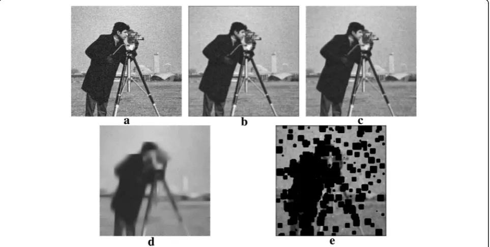
standard deviation, and the asterisk represents convolution [1]. If impulse noise is present, weighted averaging in (12) spreads the impulse noise corrupted image gradients along with noise free image gradients, as is clear from (5–7) and Fig.1e. For Laplacian or long-tailed distribution, median is the posterior estimate and, hence, the second term on the RHS of (12) is an expectation such that it is an ML estimate in theL1sense [17]. Then, it is possible to write (12) as
I uð Δx;vΔy;ðnþ1ÞΔtÞ ¼I uð Δx;vΔy;nΔtÞ
þλg Medð ½∇kIÞMed½∇kI:
ð14Þ Equation (14) describes a smooth first-order diffusion process that is robust to impulse noise or outliers with long-tailed distributions. It is first order on account of the fact that the median estimate is simply the selection of one of the first order spatial derivatives∇NI,∇SI,∇EI, and∇WI in (9) after sorting. Median sorting renders (14) optimal in the sense of the length functional [18]. A first-order space-time differential equation has an exponential impulse response, and, therefore, the weighting function or kernel function in (14) can be chosen as an exponential function
g Medð ½∇kIÞ ¼ exp:ð−ðMed½∇kI=KÞÞ; ð15Þ
where K is a constant; (15) is consistent with
first-order smoothing process. Equation (14) is free
of the spreading effect with respect to impulse noise samples on account of the elimination of impulse noise-corrupted gradients prior to smoothing. This is in contrast to the well-established mean filter [19], PDE-based diffusion smoothing filters [20], bi-lateral filters [21], and guided filters [22, 23] which
are not intrinsically robust. They require
pre-diffusion processing and elaborate post-diffusion processing for good performance in the presence of outliers [4–10, 19–23]. It is shown in Section 3 that
(14) provides smoothing, Gaussian and impulse
noise elimination, and edge preservation and is
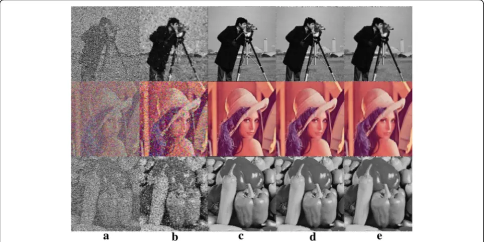
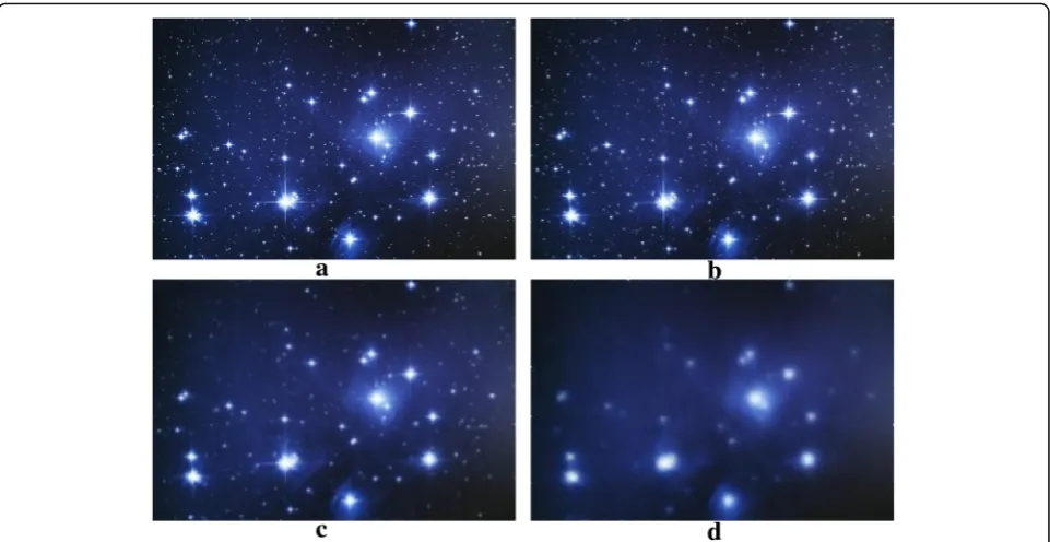
Fig. 3Performance ofaRF (λ= 0.25),bAMD (λ= 0.25),cAADF (λ= 0.25),dFORADF (λ= 0.25), andeFORADF (λ= 1) for salt and pepper noise at 70% density.λrepresents the control parameter, andnrepresents the number of iterations
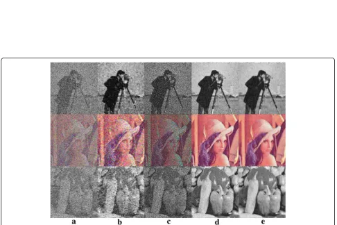
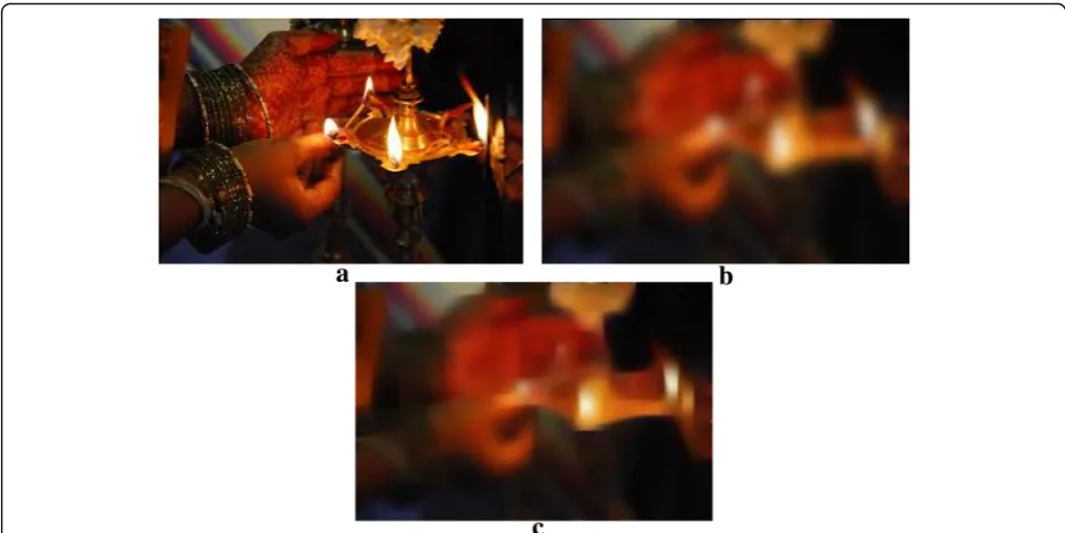
Fig. 5Performance ofaRF (λ= 0.25),bAMD (λ= 0.25),cAADF (λ= 0.25),dFORADF (λ= 0.25), andeFORADF (λ= 1) for high-density mixed noise.λrepresents the control parameter, andnrepresents the number of iterations. The results are given for high-density mixed noise, i.e., Gaussian noise of variance 0.1 plus salt and pepper noise of density 70%
intrinsically robust. We also demonstrate that (14) is the simplest in terms of arithmetic complexity. In the context of digital image processing, (14) can be algorithmically expressed as
Inþ1
i;j ¼Ini;jþλg Medð ½∇kIÞ: Med In
i−1;j−Ini;j
; In iþ1;j−Ini;j
;
In i;jþ1−Ini;j
; In i;j−1−Ini;j
2
4
3 5 8
< :
9 = ;;
ð16Þ
Inþ1
i;j ¼Ini;jþλg Med In
i−1;j−Ini;j
; In iþ1;j−Ini;j
;
In i;jþ1−Ini;j
; In i;j−1−Ini;j
2
4
3 5 8
< :
9 = ;
: Med I n i−1;j−Ini;j
; Iniþ1;j−Ini;j
;
Ini;jþ1−Ini;j
; Ini;j−1−Ini;j
2
4
3 5 8
< :
9 = ;;
ð17Þ wherei,jare spatial indices;nis the iteration number; λ is the control parameter; Ini;j represents the pixel
a
b
c
d
e
f
g
h
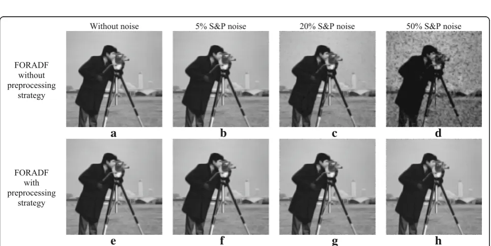
Fig. 7Performance of FORADF (λ= 1,n= 10) with and without preprocessing strategy. Without preprocessing strategy:awithout noise,b -d5%, 20%, and 50% salt and pepper noise respectively. With preprocessing strategy:ewithout noise,f-h5%, 20%, and 50% salt and pepper noise respectively.λrepresents the control parameter, andnrepresents the number of iterations
intensity of an image pixel after n iterations at the spatial location (i,j); ðIni−1;j−Ini;jÞ, ðIniþ1;j−Ini;jÞ, ðIni;jþ1−Ini;jÞ, and ðIn
i;j−1−Ini;jÞ represent first-order spatial derivatives along north, south, east, and west directions, respect-ively; and g(.) is an exponential function given by (15). Perona-Malik [2] and Canny [24] have suggested the procedure for choosing the value(s) for K. This proced-ure is followed in fixing K = 2. Algorithm (16) works well for any value of λ in the interval 0 <λ≤1 in accordance with Courant-Friedrichs-Lewy (CFL) condi-tion [25]. With 0 <λ≤1, the algorithm is an excellent
smoother as n →∞, and, therefore, the number of
time iterations can be selected on the basis of objective performance metrics and subjective visual quality.
Algorithm (17) involves the following step by step
process: with respect to an image pixel In
i;j , i.e., the center pixel, along with its four neighboring pixels along northðIn
i−1;jÞ, southðIniþ1;jÞ, eastðIni;jþ1Þ, and westðIni;j−1Þ
directions,
1. Get the four directional derivatives of the center pixel along north, south, east, and west directions by calculating the difference in pixel intensities of each neighboring pixel along that direction to that of the center pixel. Pixel padding can be used to process the first row, last row, first column, and last column image pixels.
2. Select the median value of the four directional derivatives of step 1.
3. Using the median value the directional derivatives of step 2, find the value of the weighting function using the analytical formula given in (15).
4. Select an appropriate control parameter (λ) value in between 0 and 1, which gives an optimal
performance inL1sense for the given input image. 5. Find a scalar value which is the product of the
values of step 2, step 3, and step 4.
6. To get an updated pixel intensity valueIni;þj1, add the value of step 5 to the pixel intensity of the center pixelIni;j.
7. In case of color images, the same procedure has to be extended to three image planes.
3 Results and discussion
Three foundational diffusion smoothing methods [2, 4, 5] and one extended model are considered for comparison.
The benchmark Perona-Malik algorithm [2] provides
edge-preserving Gaussian smoothing. The goal of the other two foundational diffusion smoothing methods [4, 5] is to provide image smoothing while suppressing impulse noise without affecting edge information. The state-of-the-art ex-tended model [12] is included to highlight the increased computational complexity by adding additional stages in attempting to improve the performance. The proposed
algorithm (16) is primarily a low arithmetic complexity, edge-preserving smoothing algorithm, and impulse noise removal is an additional strength of the algorithm without a requirement for additional stages. Other methods [6– 12] are the extensions or modifications of the three foun-dational methods by adding additional stages for the re-moval of impulse noise which results in high complexity and poor smoothing. However, one method [12] from [6– 12] is considered for comparison to highlight the trade-off between performance and complexity. Salt and pepper noise is included as a convenient model of strong outliers; similar results can be generated for random-valued im-pulse noise. The proposed algorithm is mainly meant for edge-preserving image smoothing at low complexity in the presence of salt and pepper noise. The results for mixed noise, i.e., mild Gaussian noise of variance 0.1 plus salt and pepper noise are also included to show that no image will ever be free of a mild Gaussian noise. This re-sult for mixed noise is only an addition. Cameraman image, Lena image, and Pepper image of size 512 × 512 are selected as test images. An additional non-iterative
simplifying strategy employed is that if the center pixel in-side the mask is an impulse corrupted pixel, it can be re-placed by an immediate neighbor pixel [26], assuming that impulse noise pixels do not occur consecutively.
Figure1a shows an image corrupted by Gaussian noise of variance 0.1. Figure1b and c show the performance of PM algorithm and the proposed first-order robust aniso-tropic diffusion filter (FORADF), respectively. The num-ber of iterations is kept low at 5. It is confirmed that
FORADF works well for Gaussian noise. Figure 1d
dem-onstrates that FORADF is a good smoother (n= 25). Fig-ure1e shows the spreading effect in PM algorithm for the image corrupted by 20% salt and pepper noise for iteration numbern= 20.
Figure2a–e show the results of the robust filter (RF;n
= 5) [5], anisotropic median diffusion (AMD; n= 5) [4], adaptive anisotropic diffusion filter (AADF; n= 1) [12], FORADF(λ= 0.25, n= 5), and FORADF(λ= 1,n= 5), re-spectively, with salt and pepper noise at 20%, for the three test images. It can be seen that AMD (K1= 0.5,λ = 0.25) gives better performance than the robust filter (λ = 0.25). The proposed FORADF (λ= 0.25 andλ= 1) out-performs the RF and AMD. It is clear from the results that FORADF is robust, preserves edge information, and is a good smoother. The performance of AADF is very good in terms of salt and pepper removal, but it is a poor smoother in comparison with FORADF. The major advantage of FORADF in comparison with AADF is very low complexity.
Table 1Performance for Gaussian noise
Methods Noise type Variance λ NI PSNR SSIM
PM GN 0.1 0.25 5 19.267 0.8287
FORADF GN 0.1 1 5 20.233 0.8384
FORADF GN 0.1 1 100 Good smoothing
GNGaussian noise,NInumber of iteration,S&Psalt and pepper noise
Figure 3a–e show the results of the RF (λ= 0.25,n= 5), AMD (λ= 0.25,n= 5), AADF (λ= 0.25,n= 1), FORADF (λ = 0.25,n= 5), and FORADF (λ= 1,n= 5), respectively, with salt and pepper noise at 70% for the three test images. The proposed filter works very well at higher noise densities and for very low number of iterations, whereas RF and
AMD fail to provide acceptable performance at
high-density salt and pepper noise with low number of iter-ations. The performance of RF [5] and AMD [4] can be im-proved by increasing the number of iterations. For acceptable performance at higher noise densities, both RF [5] and AMD [4] require the number of iterations be high (above 100), whereas FORADF performs better at much lower number of iterations. Since the focus of AADF is on salt and pepper noise removal, it works well at higher noise densities also. It is clear from the result that FORADF out-performs AADF in terms of image smoothing and compu-tational complexity.
Figure 4a–e show the results of RF (λ= 0.25, n= 5), AMD (λ= 0.25,n= 5), AADF (λ= 0.25,n= 1), FORADF (λ= 0.25,n= 5), and FORADF (λ= 1,n= 5) forn= 5, re-spectively, for the three images corrupted by mixed noise consisting of Gaussian noise of variance 0.1 plus salt and pepper noise of density 20%. The proposed FORADF works better in comparison with the other three algorithms. The non-iterative AADF is very good
in the removal of salt and pepper noise, but it fails to work even in the presence of low-density Gaussian noise; in addition, it is not a good smoother in compari-son with FORADF and is computationally complex.
Figure5a–e show the performance of the RF (λ= 0.25,
n= 5), AMD (λ= 0.25, n= 5), AADF (λ= 0.25, n= 1), FORADF (λ= 0.25, n= 5), and FORADF (λ= 1, n= 5), respectively, for the three images corrupted by mixed noise consisting of Gaussian noise of variance 0.1 plus salt and pepper noise of noise density 70%. The results show that FORADF performs well at high noise dens-ity with low number of iterations. The performance of RF and AMD are very poor at high noise density with low number of iterations. Even with the in-creased number of iterations, the performance of RF [5] and AMD [4] at high noise density are not appre-ciable. AADF is also not suitable in the presence of even mild Gaussian noise.
Figure 6a and b show the results of FORADF for the
image corrupted by mixed noise consisting of Gaussian noise of variance 0.1 and salt and pepper noise density
90% for n= 5 and n= 25, respectively. These are the
worst case results which demonstrate the intrinsic ro-bustness of FORADF.
Figure7a–d show the performance of FORADF
with-out the preprocessing strategy and Fig. 7e–h show the performance of FORADF with the preprocessing strat-egy. It is clear from Fig.7e and a that FORADF is a good image smoother with and without the preprocessing
strategy. Figure 7b and c show that FORADF is also a
good edge-preserving impulse noise suppresser at low and medium impulse noise densities even without the preprocessing strategy. The preprocessing strategy is an Table 3Performance of FORADF for very high-density mixed
noise
Methods Noise type Noise % λ NI PSNR SSIM
FORADF GN + S&P 0.1 + 90 1 5 16.338 0.8190
FORADF GN + S&P 0.1+ 90 1 25 16.825 0.8190
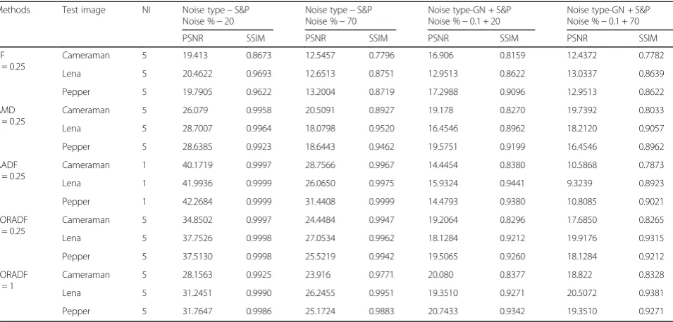
Table 2Performance for low-density salt and pepper noise
Methods Test image NI Noise type−S&P Noise %−20
Noise type−S&P Noise %−70
Noise type-GN + S&P Noise %−0.1 + 20
Noise type-GN + S&P Noise %−0.1 + 70
PSNR SSIM PSNR SSIM PSNR SSIM PSNR SSIM
RF
λ= 0.25
Cameraman 5 19.413 0.8673 12.5457 0.7796 16.906 0.8159 12.4372 0.7782
Lena 5 20.4622 0.9693 12.6513 0.8751 12.9513 0.8622 13.0337 0.8639
Pepper 5 19.7905 0.9622 13.2004 0.8719 17.2988 0.9096 12.9513 0.8622
AMD
λ= 0.25
Cameraman 5 26.079 0.9958 20.5091 0.8927 19.178 0.8270 19.7392 0.8033
Lena 5 28.7007 0.9964 18.0798 0.9520 16.4546 0.8962 18.2120 0.9057
Pepper 5 28.6385 0.9923 18.6443 0.9462 19.5751 0.9199 16.4546 0.8962
AADF
λ= 0.25
Cameraman 1 40.1719 0.9997 28.7566 0.9967 14.4454 0.8380 10.5868 0.7873
Lena 1 41.9936 0.9999 26.0650 0.9975 15.9324 0.9441 9.3239 0.8923
Pepper 1 42.2684 0.9999 31.4408 0.9999 14.4793 0.9380 10.8085 0.9021
FORADF
λ= 0.25
Cameraman 5 34.8502 0.9997 24.4484 0.9947 19.2064 0.8296 17.6850 0.8265
Lena 5 37.7526 0.9998 27.0534 0.9962 18.1284 0.9212 19.9176 0.9315
Pepper 5 37.5130 0.9998 25.5219 0.9942 19.5065 0.9260 18.1284 0.9212
FORADF
λ= 1
Cameraman 5 28.1563 0.9925 23.916 0.9771 20.080 0.8377 18.822 0.8328
Lena 5 31.2451 0.9990 26.2455 0.9951 19.3510 0.9271 20.5072 0.9381
addition for the purpose of increasing FORADF effi-ciency at higher impulse noise densities. The added pre-processing strategy does not significantly increase the computational complexity and, hence, is retained at all noise densities. Figure7h and d demonstrate a compari-son of FORADF performance with and without the pre-processing strategy at higher impulse noise density. In a practical situation, robustness implies up to 20% impulse noise, and, hence, the proposed algorithm is an excellent robust smoother even without the preprocessing strategy and is attractive for computational photography [27,28].
Figure8demonstrates the intrinsic robustness of FOR-ADF in comparison with the foundational robust
diffu-sion algorithms RF and AMD. Figure 8d shows the
excellent intrinsic robustness characteristic in addition to the anisotropic smoothing of FORADF at a very low number of iterations. Figure 9 demonstrates the aniso-tropic smoothing property of FORADF in comparison with the foundational PM algorithm. It is clearly seen from Fig. 9b and c that anisotropic smoothing behavior of FORADF is superior in terms of smoothing and edge preservation in comparison with PM algorithm.
20 22 24 26 28 30 32 34 36 38 40
= 0.25 = 0.5 = 0.75 = 1
PSNR
Values
Performannce of FORADF for various values
Cameraman Lena Pepper
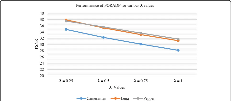
Fig. 10Performance of FORADF in terms of PSNR for variousλvalues at 20% salt and pepper noise density forn= 5.λrepresents the control parameter, andnrepresents the number of iterations. The figure shows the stability of FORADF for variousλvalues, and the performance is measured in terms of the performance metric PSNR. : performance of FORADF for Cameraman image. : performance of FORADF for Lena image. : performance of FORADF for Pepper image.
Table 4Edge Preservation Index (EPI)
Methods Test image NI Noise type−S&P
Noise %−20
Noise type−S&P Noise %−70
Noise type-GN + S&P3 Noise %−0.1 + 20
Noise type-GN + S&P3 Noise %−0.1 + 70
EPI EPI EPI EPI
RF λ= 0.25
Cameraman 5 0.4003 0.3288 0.3696 0.3316
Lena 5 0.3560 0.3565 0.3468 0.3457
Pepper 5 0.3551 0.3850 0.3520 0.3861
AMD λ= 0.25
Cameraman 5 0.4672 0.3485 0.4040 0.3363
Lena 5 0.4038 0.2490 0.3793 0.2487
Pepper 5 0.4482 0.2705 0.4173 0.2424
AADF λ= 0.25
Cameraman 1 0.8831 0.5740 0.3672 0.3356
Lena 1 0.9081 0.5811 0.4220 0.4143
Pepper 1 0.8679 0.5313 0.4134 0.4209
FORADF λ= 0.25
Cameraman 5 0.8495 0.5391 0.4064 0.3297
Lena 5 0.8071 0.4870 0.4340 0.3243
The peak signal to noise ratio (PSNR) and the struc-tural similarity index metric (SSIM), listed in Tables1,2,
and 3, clearly demonstrate the superiority of FORADF
in terms of noise removal and edge-preserving image smoothing. Even though AADF shows slightly better performance than FORADF in terms of PSNR and SSIM for 20% and 70% salt and pepper noise densities (Table2), AADF fails to perform even in the presence of low-density Gaussian noise and AADF is not a smoother; in addition, AADF, which is non-iterative re-quiring one-shot solution, is computationally complex.
Table 4 shows the performance of various filters in
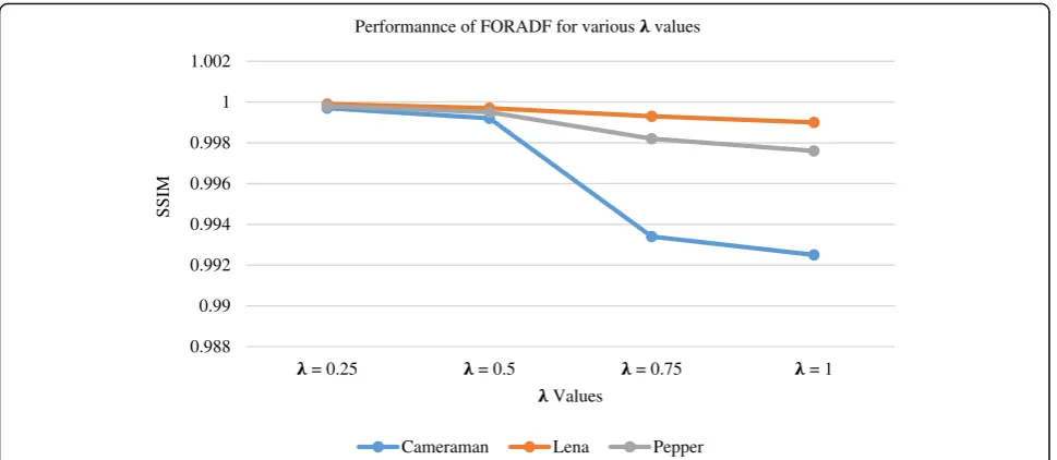
terms of edge preservation index (EPI). Figures 10 and
11show the performance of FORADF forλ values 0.25,
0.5, 0.75, and 1 in terms of the performance metrics PSNR and SSIM, respectively. The results are obtained for the input images corrupted by 20% salt and pepper noise density, and the number of iterations is chosen as
n= 5. It is clear from Figs.10and11that FORADF pvides very good performance in terms of intrinsic
ro-bustness, smoothing, and edge preservation over all λ
values in the interval (0, 1]. In real-time DSP, which does not always mean high speed [29], multipliers and adders determine the computational efficiency [30] and hard-ware complexity [31] which is an important
consider-ation in meeting power budgets [29]. A typical
comparison from this perspective is presented in Table5. Computational efficiency of FORADF in comparison with RF and AMD is expressed in terms of percentage excess/savings on arithmetic complexity (C) where Cref,
CAMD, andCRFrepresent the complexity of the reference FORADF, AMD, and RF, respectively, as the number of arithmetic operations per pixel per iteration. In RF, 41.37% excess arithmetic computations are required in comparison with FORADF to perform one pixel
oper-ation. Similarly, 75.36% excess computations are
Table 5Hardware complexity in DSP context
Methods Noise type
Noise %
λ NIAP No. of A/M/S per iteration (C)
Running time per iteration in seconds
Running time for NIAP in seconds*
Computational efficiency of FORADF (Cref) in
comparison with RF and AMD in terms of excess/ savings onC(%)
((C−Cref)/C)
RF GN +
S&P 0.1 + 70
0.25 100 11/18/0 3.5244 352.44 ((CRF−Cref)/CRF)= 41.37% excess
AMD GN +
S&P 0.1 + 70
0.25 100 12/33/24 5.5495 554.95 ((CAMD−Cref)/CAMD)= 75.36% excess
FORADF GN +
S&P 0.1 + 70
1 5 5/4/8 4.9407 24.7038 ((Cref−Cref)/Cref)= 0% excess
A/M/S additions/multiplications/sorting,NIAPnumber of iterations required for acceptable performance,Carithmetic complexity *MATLAB R2014a, 567u7 Intel (R) core (TM) i5-5200 U CPU @ 2.20 GHz, 64—bit Operating System, RAM-4.00 GB
0.988 0.99 0.992 0.994 0.996 0.998 1 1.002
= 0.25 = 0.5 = 0.75 = 1
SSIM
Values
Performannce of FORADF for various values
Cameraman Lena Pepper
required in AMD in comparison with FORADF to per-form one pixel operation. The total number of multi-pliers and adders is the lowest for FORADF; in the context of DSP, this spirals down to power efficiency, since multipliers are power guzzlers [31]. The lowest number of iterations of FORADF compensates for the increased running time due to sorting. Therefore, the total energy consumed by FORADF is lower than that of AMD and is comparable with that of RF. The results clearly demonstrate that FORADF is an efficient edge-preserving robust smoothing in comparison with the four filters for Gaussian, salt and pepper, and mixed noise situations across all noise densities, and, hence, FORADF is significant in the context of power-efficient implementations.
4 Conclusion
Diffusion smoothing of images with edge preservation in robust environment is a growing area of research. Exist-ing robust diffusion smoothExist-ing filters employ two or more stages and are generally complex in terms of arith-metic operations. A low aritharith-metic complexity model and an algorithm for robust diffusion smoothing of im-ages are derived. The algorithm exhibits superior per-formance in terms of standard perper-formance criteria and visual results in Gaussian, impulse, and mixed noise situ-ations. The intrinsic computational simplicity of the pro-posed model and algorithm are significant in the context of power efficient implementations.
Abbreviations
AADF:Adaptive anisotropic diffusion filter; AMD: Anisotropic median diffusion; CFL: Courant-Friedrichs-Lewy; DSP: Digital signal processing; ENI: Edge pixels, noisy pixels, and image pixels; EPI: Edge preservation index; FORADF: First-order robust anisotropic diffusion filter; GN: Gaussian noise; LHS: Left hand side; ML: Maximum likelihood; NI: Number of iteration; NIAP: Number of Iterations required for Acceptable Performance; PDE: Partial differential equation; PM: Perona-Mailk algorithm; PSNR: Peak signal to noise ratio; RF: Robust filter; RHS: Right hand side; S&P: Salt and pepper noise; SSIM: Structural similarity index metric
Acknowledgements Not Applicable.
Funding
This work was not supported by any funding.
Availability of data and materials
Data sharing not applicable to this article as no datasets were generated or analyzed during the current study.
Authors’contributions
DE contributed to the conceptual and theoretical formulations. NRR contributed to the algorithm development, programming, and validation. RS contributed to the computing platforms and methodology. All authors read and approved the final manuscript.
Authors’information
Resmi R. Nair received AMIE degree in Electronics and Communication Engineering from The Institution of Engineers (India) in 2007 and she received M.E degree in VLSI Design from Anna University in 2009. She is a research scholar of Anna University, Chennai, India. Her research interests
include Digital Signal Processing, Digital Image Processing, and VLSI. She is a member of IEEE, IETE, and ISTE (India).
Ebenezer David obtained his Ph. D degree in communication engineering from Anna University, Chennai, India in 1994. He is a Professor Emeritus in the Department of Electronics and Communication Engineering, College of Engineering, Anna University, Chennai. His research publications are in the area of nonlinear digital filtering with well over 45 journal and conference publications and 1200 citations. He has also delivered keynote speeches in international conferences. He served as a referee for journal of Medical Engineering and physics (U.K), IET, IEEE Transactions on Image Processing, and JEI (U.S.A). He is an elected AMIE (India), a member of ISTE (India), and a senior member IEEE.
Sivakumar Rajagopal is a Professor and Head of Department of Electronics and Communication Engineering at RMK Engineering College, Tamil Nadu, India. He has been teaching in the Electronics and Communication field since 1997. He obtained his Master’s degree and Ph. D from College of Engineering Guindy, Anna University, Chennai. His research interests include Bio Signal Processing, Medical Image Processing, wireless body sensor networks and VLSI. He has published over 34 journal and 42 conference papers. He has chaired a number of international conferences and has delivered keynote speeches Dr. Siva is a life member of the Indian Society of Technical Education, a senior member of IEEE.
Competing interests
The authors declare that they have no competing interests.
Publisher’s Note
Springer Nature remains neutral with regard to jurisdictional claims in published maps and institutional affiliations.
Author details 1
Department of Electronics and Communication Engineering, RMK Engineering College, Kavaripettai, Tamil Nadu 601206, India.2Department of Electronics and Communication Engineering, Anna University, Chennai, Tamil Nadu 600025, India.
Received: 1 July 2017 Accepted: 15 February 2019
References
1. J. Babaud, A. Witkin, M. Baudin, R. Duda, Uniqueness of the Gaussian kernel for scale space filtering. IEEE Trans. Pattern Anal. Mach. Intell.8(1), 26–33 (1986)
2. P. Perona, J. Malik, Scale space and edge detection using anisotropic diffusion. IEEE Trans. Pattern Anal. Mach. Intell.12(7), 629–639 (1990) 3. M.J. Black, D.H. Marimont, Robust anisotropic diffusion. IEEE Trans. Image
Process.7(3), 421–432 (1998)
4. J. Ling, A.C. Bovik, Smoothing low-SNR molecular images via anisotropic median diffusion. IEEE Trans. Med. Imag.12(4), 377–383 (2002)
5. B. Ham, D. Min, K. Sohn, Robust scale space filter using second order partial differential equations. IEEE Trans. Image Process.21(9), 3937–3951 (2012) 6. J. Wu, C. Tang, PDE-based random-valued impulse noise removal based on
new class of controlling functions. IEEE Trans. Image Process.20(9), 2428– 2438 (2011)
7. W. Wang, P. Lu, IEEEProceedings of the 10th world congress on intelligent
control and automation. Adaptive Switching Anisotropic Diffusion Model for
Universal Noise Removal (Beijing, 2012), pp. 4803–4808
8. X. Chen, C. Tang, X. Yan, Switching degenerate diffusion PDE filter based on impulse like probability for universal noise removal. Elsevier Int. J. Electron. Commun.68(9), 851–857 (2014)
9. N.U. Khan, K.V. Arya, M. Pattanaik, Edge preservation of impulse noise filtered images by improved anisotropic diffusion, Springer Sci. + Bus. Media New York. Multimed. Tools Appl.73(1), 573–597 (2014)
10. H. Tian, H. Cai, J. Lai, A novel diffusion system for impulse noise removal based on a robust diffusion tensor. Elsevier Neurocomputing133, 222–230 (2014)
11. S.I. Cho, S.J. Kang, H.S. Kim, Y.H. Kim, Dictionary-based anisotropic diffusion for noise reduction. Elsevier Pattern Recogn. Lett.46, 36–45 (2014) 12. T. Veerakumar, S. Esakkirajan, I. Vennila, Edge preservation adaptive
13. B. Marami, B. Scherrer, O. Afacan, B. Erem, S.K. Warfield, A. Gholipour, Motion-robust diffusion-weighted brain MRI reconstruction through slice-level registration-based motion tracking. IEEE Trans. Med. Imag.35(10), 2258–2269 (2016)
14. A Einstein, Investigation on the Theory of the Brownian Movement, ed. By R Furth and Transl. by AD Cowper (Dover Publications, New York, 1956), pp. 9–15
15. M.H. Hayes,Statistical Digital Signal Processing and Modelling(Wiley, Wiley-India, New Delhi, 2011), pp. 99–102
16. K. Kim, G. Shevlyakov, Why Gaussianity [an attempt to explain this phenomenon]. IEEE Signal Process. Mag.25(2), 112 (2008)
17. J. Astola, P. Kuosmanen,Fundamentals of Nonlinear Digital Filtering(CRC Press, New York, 1997), p. 40
18. P.J. Huber,Robust Statistics, 2nd edn. (Wiley, New Jersey, 2009), p. 46 19. S. Rakshit, A. Ghosh, B.U. Shankar, Fast mean filtering technique (FMFT).
Elsevier Pattern Recogn.40(3), 890–897 (2007)
20. J. Weickert,Anisotropic Diffusion in Image Processing(BG Teubner, Stuttgart, 2008), pp. 1–26
21. S. Paris, P. Kornprobst, J. Tumblin, F. Durand,Bilateral Filtering(Theory and Applications, (now Publishers, USA, 2009), pp. 5–9
22. K. He, J. Sun, X. Tang, Guided image filtering. IEEE Trans. Pattern Anal. Mach. Intell.35(6), 1397–1409 (2013)
23. L. Caraffa, J.P. Tarel, P. Charbonnier, The guided bilateral filter: when the joint/cross bilateral filter becomes robust. IEEE Trans. Image Process.24(4), 1199–1208 (2015)
24. J. Canny, A computational approach to edge detection. IEEE Trans. Pattern Anal. Mach. Intell.8, 679–698 (1986)
25. R. Courant, K. Friedrichs, H. Lewy, Uber die partiellen
Differenzengleichungen der mathematischen Physik. Math. Ann.100, 32–74 (1928) (Trans.: in L. English byPD Lax, Hyperbolic difference equations: a review of the courant-friedrichs-lewy paper in the light of recent developments, IBM J. of Res. and Develop., 11(2), 235–238(1967) 26. K.S. Srinivasan, D. Ebenezer, A new fast and efficient decision-based
algorithm for removal of high-density impulse noises. IEEE Signal Process. Lett.14(3), 189–192 (2007)
27. R. Ramanath, W.E. Snyder, Y. Yoo, M.S. Drew, Color image processing pipeline. IEEE Signal Process. Mag.22(1), 34–43 (2005)
28. W. van Houten, Z. Geradts, Using anisotropic diffusion for efficient extraction of sensor noise in camera identification. J. Forensic Sci.57(2), 521–527 (2012)
29. P. Deodar,Dissertation, University of Cincinnati(2014)
30. H.K. Garg,Digital Signal Processing Algorithms: Number Theory, Convolution,
Fast Fourier Transforms, and Application(CRC Press, Florida, 1998), p. 1