R E S E A R C H
Open Access
Research on image classification model
based on deep convolution neural network
Mingyuan Xin
1and Yong Wang
2*Abstract
Based on the analysis of the error backpropagation algorithm, we propose an innovative training criterion of depth neural network for maximum interval minimum classification error. At the same time, the cross entropy and M3CE are analyzed and combined to obtain better results. Finally, we tested our proposed M3 CE-CEc on two deep
learning standard databases, MNIST and CIFAR-10. The experimental results show that M3CE can enhance the
cross-entropy, and it is an effective supplement to the cross-entropy criterion. M3 CE-CEc has obtained good results in both databases.
Keywords: Convolution neural network, Image classification, M3CE-CEc
1 Introduction
Traditional machine learning methods (such as multi-layer perception machines, support vector machines, etc.) mostly use shallow structures to deal with a limited number of samples and computing units. When the tar-get objects have rich meanings, the performance and generalization ability of complex classification problems are obviously insufficient. The convolution neural net-work (CNN) developed in recent years has been widely used in the field of image processing because it is good at dealing with image classification and recognition problems and has brought great improvement in the ac-curacy of many machine learning tasks. It has become a powerful and universal deep learning model.
Convolutional neural network (CNN) is a multilayer neural network, and it is also the most classical and common deep learning framework. A new reconstruc-tion algorithm based on convolureconstruc-tional neural networks is proposed by Newman et al. [1] and its advantages in speed and performance are demonstrated. Wang et al. [2] discussed three methods, that is, the CNN model with pretraining or fine-tuning and the hybrid method. The first two executive images are passed to the network one time, while the last category uses a patch-based fea-ture extraction scheme. The survey provides a milestone
in modern case retrieval, reviews a wide selection of dif-ferent categories of previous work, and provides insights into the link between SIFT and the CNN based ap-proach. After analyzing and comparing the retrieval per-formance of different categories on several data sets, we discuss a new direction of general and special case re-trieval. Convolution neural network (CNN) is very inter-ested in machine learning and has excellent performance in hyperspectral image classification. Al-Saffar et al. [3] proposed a classification framework called region-based pluralistic CNN, which can encode semantic context-aware representations to obtain promising features. By combining a set of different discriminant appearance factors, the representation based on CNN presents the spatial spectral contextual sensitivity that is essential for accurate pixel classification. The proposed method for learning contextual interaction features using various region-based inputs is expected to have more discrimin-ant power. Then, the combined representation contain-ing rich spectrum and spatial information is fed to the fully connected network and the label of each pixel vec-tor is predicted by the Softmax layer. The experimental results of the widely used hyperspectral image datasets show that the proposed method can outperform any other traditional deep-learning-based classifiers and other advanced classifiers. Context-based convolution neural network (CNN) with deep structure and pixel-based multilayer perceptron (MLP) with shallow structure are recognized neural network algorithms * Correspondence:[email protected]
2Heihe University, No. 1 Xueyuan Road education science and technology
zone, Heihe, Heilongjiang, China
Full list of author information is available at the end of the article
which represent the most advanced depth learning methods and classical non-neural network algorithms. The two algorithms with very different behaviors are in-tegrated in a concise and efficient manner, and a rule-based decision fusion method is used to classify very fine spatial resolution (VFSR) remote sensing im-ages. The decision fusion rules, which are mainly based on the CNN classification confidence design, reflect the usual complementary patterns of each classifier. There-fore, the ensemble classifier MLP-CNN proposed by Said et al. [4] acquires supplementary results obtained from CNN based on deep spatial feature representation and MLP based on spectral discrimination. At the same time, the CNN constraints resulting from the use of convolution filters, such as the uncertainty of object boundary segmentation and the loss of useful fine spatial resolution details, are compensated. The validity of the ensemble MLP-CNN classifier was tested in urban and rural areas using aerial photography and additional satel-lite sensor data sets. MLP-CNN classifier achieves prom-ising performance and is always superior to pixel based MLP, spectral and texture based MLP, and context-based CNN in classification accuracy. The research paves the way for solving the complex problem of VFSR image classification effectively. Periodic inspection of nuclear power plant components is important to ensure safe op-eration. However, current practice is time-consuming, tedious, and subjective, involving human technicians examining videos and identifying reactor cracks. Some vision-based crack detection methods have been devel-oped for metal surfaces, and they generally perform poorly when used to analyze nuclear inspection videos. Detecting these cracks is a challenging task because of their small size and the presence of noise patterns on the surface of the components. Huang et al. [5] proposed a depth learning framework based on convolutional neural network (CNN) and Naive Bayes data fusion scheme (called NB-CNN), which can be used to analyze a single video frame for crack detection. At the same time, a new data fusion scheme is proposed to aggregate the information extracted from each video frame to en-hance the overall performance and robustness of the sys-tem. In this paper, a CNN is proposed to detect the fissures in each video frame, the proposed data fusion scheme maintains the temporal and spatial coherence of the cracks in the video, and the Naive Bayes decision ef-fectively discards the false positives. The proposed framework achieves a hit rate of 98.3% 0.1 false positives per frame which is significantly higher than the most advanced method proposed in this paper. The prediction of visual attention data from any type of media is valuable to content creators and is used to drive coding algorithms effectively. With the current trend in the field of virtual reality (VR), the adaptation of known
technologies to this new media is beginning to gain mo-mentum R. Gupta and Bhavsar [6] proposed an exten-sion to the architecture of any convolutional neural network (CNN) to fine-tune traditional 2D significant prediction to omnidirectional image (ODI). In an end-to-end manner, it is shown that each step in the pipeline presented by them is aimed at making the gen-erated salient map more accurate than the ground live data. Convolutional neural network (Ann) is a kind of depth machine learning method derived from artificial neural network (Ann), which has achieved great success in the field of image recognition in recent years. The training algorithm of neural network is based on the error backpropagation algorithm (BP), which is based on the decrease of precision. However, with the increase of the number of neural network layers, the number of weight parameters will increase sharply, which leads to the slow convergence speed of the BP algorithm. The training time is too long. However, CNN training algo-rithm is a variant of BP algoalgo-rithm. By means of local connection and weight sharing, the network structure is more similar to the biological neural network, which not only keeps the deep structure of the network, but also greatly reduces the network parameters, so that the model has good generalization energy and is easier to train. This advantage is more obvious when the network input is a multi-dimensional image, so that the image can be directly used as the network input, avoiding the complex feature extraction and data reconstruction process in traditional recognition algorithm. Therefore, convolutional neural networks can also be interpreted as a multilayer percep-tron designed to recognize two-dimensional shapes, which are highly invariant to translation, scaling, tilting, or other forms of deformation [7–15].
the rich spatial information of HSI, which has been proved to be beneficial to classification tasks. Yan et al. [16] proposed a space and class structure regularized sparse representation (SCSSR) graph for semi-supervised HSI classification. Specifically, spatial information has been incorporated into the SR model through graph La-place regularization, which assumes that spatial neigh-bors should have similar representation coefficients, so the obtained coefficient matrix can more accurately re-flect the similarity between samples. In addition, they also combine the probabilistic class structure (which means the probabilistic relationship between each sam-ple and each class) into the SR model to further improve the differentiability of graphs. Hyion and AVIRIS hyper-spectral data show that our method is superior to the most advanced method. The invariance extracted by Zhang et al. [17], such as the specificity of uniform samples and the invariance of rotation invariance, is very important for object detection and classification applica-tions. Current research focuses on the specific invariance of features, such as rotation invariance. In this paper, a new multichannel convolution neural network (mCNN) is proposed to extract the invariant features of object classification. Multi-channel convolution sharing the same weight is used to reduce the characteristic variance of sample pairs with different rotation in the same class. As a result, the invariance of the uniform object and the rotation invariance are encountered simultaneously to improve the invariance of the feature. More importantly, the proposed mCNN is particularly effective for small training samples. The experimental results of two datum datasets for handwriting recognition show that the pro-posed mCNN is very effective for extracting invariant features with a small number of training samples. With the development of big data era, convolutional neural network (CNN) with more hidden layers has more com-plex network structure and stronger feature learning and feature expression ability than traditional machine learn-ing methods. Since the introduction of the convolutional neural network model trained by the deep learning algo-rithm, significant achievements have been made in many large-scale recognition tasks in the field of computer vi-sion. Chaib et al. [18] first introduced the rise and devel-opment of deep learning and convolution neural network and summarized the basic model structure, convolution feature extraction, and pool operation of convolution neural network. Then, the research status and development trend of convolution neural network model based on deep learning in image classification are reviewed, and the typical network structure, training method, and performance are introduced. Finally, some problems in the current research are briefly summarized and discussed, and new directions of future development are predicted. Computer diagnostic technology has
played an important role in medical diagnosis from the beginning to now. Especially, image classification tech-nology, from the initial theoretical research to clinical diagnosis, has provided effective assistance for the diag-nosis of various diseases. In addition, the image is the concrete image formed in the human brain by the ob-jective things existing in the natural environment, and it is an important source of information for a human to obtain the knowledge of the external things. With the continuous development of computer technology, the general object image recognition technology in natural scene is applied more and more in daily life. From image processing technology in simple bar code recognition to text recognition (such as handwritten character recogni-tion and optical character recognirecogni-tion OCR etc.) to bio-metric recognition (such as fingerprint, sound, iris, face, gestures, emotion recognition, etc.), there are many suc-cessful applications. Image recognition (Image Recogni-tion), especially (Object Category Recognition) in natural scenes, is a unique skill of human beings. In a complex natural environment, people can identify concrete objects (such as teacups) at a glance (swallow, etc.) or a specific category of objects (household goods, birds, etc.). How-ever, there are still many questions about how human be-ings do this and how to apply these related technologies to computers so that they have humanoid intelligence. Therefore, the research of image recognition algorithms is still in the fields of machine vision, machine learning, depth learning, and artificial intelligence [19–24].
Therefore, this paper applies the advantage of depth mining convolution neural network to image classifica-tion, tests the loss function constructed by M3CE on two depth learning standard databases MNIST and CIFAR-10, and pushes forward the new direction of image classification research.
2 Proposed method
Image classification is one of the hot research directions in computer vision field, and it is also the basic image classification system in other image application fields, which is usually divided into three important parts: image preprocessing, image feature extraction and classifier.
2.1 The ZCA process is shown as below
In this process, we first use PCA to zero the mean value. In this paper, we assume that X represents the image
vector [25]:μ¼ 1 m
P j¼1 m
xj
xj¼xj−μ;j¼1;2;3;⋯;m; ð1Þ
X
¼ 1
m Xm
j¼1
xjxjT ð2Þ
where I represents the covariance matrix, I is decom-posed by SVD [26], and its eigenvalues and correspond-ing eigenvectors are obtained.
U;S;V
½ ¼SVDX ð3Þ
Of which,Uis the eigenvector matrix of ∑, andSis the eigenvalue matrix of∑. Based on this,xcan be whitened by PCA, and the formula is:
xPCAwhiten¼S− 1
2UTx ð4Þ
SoXZCAwhitencan be expressed as
xZCAwhiten¼UxPCAwhiten ð5Þ
For the data set in this paper, because the training sample and the test sample are not well distinguished [27], the random generation method is used to avoid the subjective color of the artificial classification.
2.2 Image feature extraction based on time-frequency composite weighting
Feature extraction is a concept in computer vision and image processing. It refers to the use of a computer to extract image information and determine whether the points of each image belong to an image feature extrac-tion. The purpose of feature extraction is to divide the points on the image into different subsets, which are often isolated points, a continuous curve, or region. There are usually many kinds of features to describe the image. These features can be classified according to dif-ferent criteria, such as point features, line features, and regional characteristics according to the representation of the features on the image data. According to the re-gion size of feature extraction, it can be divided into two categories: global feature and local feature [24]. The image features used in some feature extraction methods in this paper include color feature and texture feature, analysis of the current situation of corner feature, and edge feature.
The time-frequency composite weighting algorithm for multi-frame blurred images is a frequency-domain and time-domain weighting simultaneous processing algo-rithm based on blurred image data. Based on the weighted characteristic of the algorithm and the feature extraction of target image in time domain and frequency domain, the depth extraction technique is based on the time-frequency composite weighting of night image to extract the target information from depth image. The main steps of the time-frequency composite weighted feature extraction method are as follows:
Step 1: Construct a time-frequency composite weighted signal model for multiple blurred images, as the following expression shows:
g tð Þ ¼pffiffisf tð½−τÞ ð6Þ
Of which,f(t) is original signal, S= (c−v)/(c+v), called the image scale factor. Referred to as scale, it represents the signal scaling change of the original image time-frequency composite weighting algorithm.pffiffiffiSis the normalized factor of image time-frequency composite weighting algorithm.
Step 2: Map the one-dimensional function to the two-dimensional functiony(t) of the time scaleaand the time shift b, and perform a time-frequency composite weighted transform on the continuous nighttime image of the image time-frequency composite weighted 0 using the square integrable function as shown below:
Wψy a;ð bÞ ¼ y;ψa;b
D E
¼
Z þ∞
−∞
y tð Þ ffiffiffiffiffiffiffiffi1
jaj
p ψ t−b
a
dt
ð7Þ
Of which, divisor 1=pffiffiffiffiffiffiffiffijaj. The energy normalization of the unitary transformation is ensured.ψa,bisψ(t) ob-tained by transformingU(a,b) through the affine group, as shown by the following expression:
ψa;bð Þ ¼t ½U a;ð bÞψð Þt ¼
1
ffiffiffiffiffiffiffiffi
jaj
p ψ t−b
a
ð8Þ
Step 3: Substituting the variable of the original image
f(t)by a= 1/s and b=τ and rewriting the expression to obtain an expression:
fs;τð Þ ¼t ½Uð1=s;τÞf tð Þ ¼pffiffiffiffiffiffiffijsjf s tðð−τÞÞ ð9Þ
Step 4: Build a multi-frame fuzzy image
time-frequency composite weighted signal form.
u tð Þ ¼ 1ffiffiffiffi T
p rect t
T exp −j 2πk ln 1− t t0
ð10Þ
Of which, rect(t) = 1 and∣t∣ ≤1/2.
Step 5: The frequency modulation law of the time-frequency composite weighted signal of multi-thread fuzzy image is a hyperbolic function;
fið Þ ¼t K t0−t;
jtj ≤T
2 ð11Þ
Step 6: Use the image transformation formula of the multi-detector fuzzy image time-frequency composite weighted signal to carry on the time-frequency compos-ite weighting to the image, the definition of the image transformation is like the formula.
wuu a;ð bÞ ¼ej2πklna
K ffiffiffi a
p ð12Þ
(
aej2πfaminðb−baÞ
fmin −
ej2πfmaxðb−baÞ
fmax
" #
þj2πðb−baÞ½Eiðj2πfmax
b−ba
ð ÞÞ−Eiðj2πfmin
a ðb−baÞg
ð13Þ
Of which, ba ¼ ð1−aÞðafm1ax− T
2Þ, and Ei(•) represents
an exponential integral.
Final output image time-frequency composite weighted image signalWuu(a,b). Therefore, compared with the traditional time-domain,c extraction technique of image features can be better realized by the time-frequency composite weighting algorithm.
2.3 Application of deep convolution neural network in image classification
After obtaining the feature vectors from the image, the image can be described as a vector of fixed length, and then a classifier is needed to classify the feature vectors.
In general, a common convolution neural network consists of input layer, convolution layer, activation layer, pool layer, full connection layer, and final output layer from input to output. The convolutional neural network layer establishes the relationship between different com-putational neural nodes and transfers input information layer by layer, and the continuous convolution-pool structure decodes, deduces, converges, and maps the feature signals of the original data to the hidden layer feature space [28]. The next full connection layer classi-fies and outputs according to the extracted features.
2.3.1 Convolution neural network
Convolution is an important analytical operation in mathematics. It is a mathematical operator that gener-ates a third function from two functions fand g, repre-senting the area of overlap between function f and function gthat has been flipped or translated. Its calcu-lation is usually defined by a following formula:
z tð Þdef¼ f tð Þ g tð Þ ¼ X þ∞
τ¼−∞
fð Þτ g tð−τÞ ð14Þ
Its integral form is the following:
z tð Þ ¼ f tð Þ g tð Þ ¼ Z þ∞
−∞ fð Þτ g tð−τÞdτ ¼
Z þ∞
−∞ f tð−τÞgð Þτdτ ð15Þ
In image processing, a digital image can be regarded as a discrete function of a two-dimensional space, de-noted as f (x, y). Assuming the existence of a two-dimensional convolution function g (x, y), the out-put image z (x, y) can be represented by the following formula:
z xð ;yÞ ¼f xð ;yÞ g xð ;yÞ ð16Þ
In this way, the convolution operation can be used to extract the image features. Similarly, in depth learning applications, when the input is a color image containing RGB three channels, and the image is composed of each pixel, the input is a high-dimensional array of 3 × image width × image length; accordingly, the kernel (called
“convolution kernel”in the convolution neural network) is defined in the learning algorithm as the accounting. Computational parameter is also a high-dimensional array. Then, when two-dimensional images are input, the corresponding convolution operation can be expressed by the following formula:
z x;ð yÞ ¼f x;ð yÞ g x;ð yÞ ¼X
t
X
h
f t;ð hÞg xð −t;y−hÞ
ð17Þ
The integral form is the following:
z xð ;yÞ ¼f xð ;yÞ g xð ;yÞ ¼∬f tð;hÞg xð −t;y−hÞdtdh
ð18Þ
If a convolution kernel ofm×nis given, there is
z x;ð yÞ ¼f x;ð yÞ g x;ð yÞ ¼X
t¼m
t¼0 Xh¼n
h¼0
f t;ð hÞg xð −t;y−hÞ
ð19Þ
Assuming that the number of convolution kernels isK, the output of the original image obtained by the above convolution operation isk∗(M−n+ 1)∗(M−n+ 1). The output is the number of convolution kernels × the image width after convolution × the image length after convolution.
2.3.2 M3CE constructed loss function
In the process of neural network training, the loss func-tion is the evaluafunc-tion standard of the whole network model. It not only represents the current state of the network parameters, but also provides the gradient of the parameters in the gradient descent method, so the loss function is an important part of the deep learning training. In this paper, we introduce the loss function proposed by M3CE. Finally, the loss function of M3CE and cross-entropy is obtained by gradient analysis.
According to the definition of MCE, we use the output of Softmax function as the discriminant function. Then, the error classification metric formula is redefined as.
dkð Þ ¼Z −pkþpq¼−
expZk
PK
j¼1 expZj
þPKexpZq j¼1 expZj
ð20Þ
Where k is the label of the sample, q= arg maxl≠k,Pl represents the most confusing class of output of the Softmax function. If we use the logistic loss function, we can find the gradient of the loss function toZ.
∂ℓkð Þdk
∂Z
¼∂ℓkð Þdk
∂dkð Þz
∂dkð Þz
∂z
¼aℓkð1−ℓkÞ ∂
dkð Þz
∂Z
ð21Þ
This gradient is used in the backpropagation algorithm to get the gradient of the entire network, and it is worth noting that if zis misdivided,ℓkwill be infinitely close to 1, and aℓk(1−ℓk) will be close to 0. Then, the gradient will be close to 0, which will cause almost no gradient to be reversed to the previous layer, which will not be good for the completion of the training process [29].
The sigmoid function is used in the traditional neural network activation function. But this is also the case during training. The observation formula shows that when the activation value is high the backpropagation gradient is very small which is called saturation. In the past, the influence of shallow neural networks was not very large, but with the increase of the number of net-work layers, this situation would affect the learning of the whole network. In particular, if the saturated sigmoid function is at a higher level, it will affect all the previous low-level gradients. Therefore, in the present depth neural networks, an unsaturated activation function
linear rectifier unit (Rectified Linear Unit, Re LU) is used to replace the sigmoid function. It can be seen from the formula that when the input value is positive, the gradi-ent of the linear rectifying unit is 1, so the gradigradi-ent of the upper layer can be reversely transmitted to the lower layer without attenuation. The literature shows that lin-ear rectification units can accelerate the training process and prevent gradient dispersion.
According to the fact that the saturation activation function in the middle of the network is not conducive to the training of the depth network, but the saturation function in the top loss function, has a great influence on the depth neural network.
ℓkð Þ ¼dk max 0ð ;1þdkÞ ð22Þ
We call it the max-margin loss, where the interval is defined as∈k= −dk(z) =Pk−Pq.
Since Pk is a probability, that is, Pk∈[0, 1], then dk∈ [−1, 1], when a sample gradually becomes misclassified from the correct classification, dk increases from −1 to 1, compared to the original logistic loss function, and even if the sample is seriously misclassified, the loss function still get the biggest loss value. Because of1 +
dk≥0, it can be simplified.
ℓkð Þ ¼dk 1þdk ð23Þ
When we need to give a larger loss value to the wrong classification sample, the upper formula can be extended to
ℓkð Þ ¼dk ð1þdkÞγ ð24Þ
where γ is a positive integer. If γ= 2 is set, we get the squared maximum interval loss function. If the function is to be applied to training deep neural networks, the gradient needs to be calculated and obtained according to the chain rule.
∂ℓkð Þdk
∂Z ¼γ
1þdk
ð Þγ−1∂dkð Þz
∂z ð25Þ
Here, we need to discuss (1) when the dimension is the dimension corresponding to the sample label, (2) when the dimension is the dimension corresponding to the confused category label, and (3) when the dimension is neither the sample label nor the dimension corre-sponding to the confused category label. The following conclusions have been drawn:
∂dkð Þz
∂Zj
¼
pj∈k;j≠k;q
pjð∈k−1Þ;j¼k
pjð∈kþ1Þ;j¼q
8 <
3 Experimental results
3.1 Experimental platform and data preprocessing MNIST (Mixed National Institute of Standards and Technology) database is a standard database in machine learning. It consists of ten types of handwritten digital grayscale images, of which 60,000 training pictures are tested with a resolution of 28 × 28.
In this paper, we mainly use ZCA whitening to process the image data, such as reading the data into the array and reforming the size we need (Figs. 1, 2, 3, 4, and 5). The image of the data set is normalized and whitened respectively. It makes all pixels have the same mean value and variance, eliminates the white noise problem in the image, and eliminates the correlation between pixels and pixels.
At the same time, a common way to change the results of image training is a random form of distortion, crop-ping, or sharpening the training input, which has the ad-vantage of extending the effective size of the training data, thanks to all possible changes in the same image. And it tends to help network learning to deal with all distortion problems that will occur in the real use of classifiers. Therefore, when the training results are ab-normal, the images will be deformed randomly to avoid the large interference caused by individual abnormal im-ages to the whole model.
3.2 Build a training network
Classification algorithm is a relatively large class of algo-rithms, and image classification algorithm is one of them. Common classification algorithms are support vector machine, k-nearest algorithm, random forest, and so on. In image classification, support vector machine (SVM) based on the maximum boundary is the most widely used classification algorithm, especially the sup-port vector machine (SVM) which uses kernel tech-niques. Support vector machine (SVM) is based on VC dimension theory and structural risk minimization the-ory. Its main purpose is to find the optimal classification hyperplane in high dimensional space so that the classi-fication spacing is in maximum and the classiclassi-fication error rate is minimized. But it is more suitable for the case where the feature dimension of the image is small and the amount of data is large after extracting the spe-cial vector.
Another commonly used target recognition method is the depth learning model, which describes the image by hierarchical feature representation. The
mainstream depth learning networks include con-strained Boltzmann machine, depth belief network foot, automatic encoder, convolution neural network, biological model, and so on. We tested the proposed M3 CE-CEc. We design different convolution neural networks for different datasets. The experimental settings are as follows: the weight parameters are ini-tialized randomly, the bias parameters are set as con-stants, the basic learning rate is set to 0.01, and the impulse term is set to 0.9. In the course of training, when the error rate is no longer decreasing, the learning rate is multiplied by 0.1.
3.3 Image classification and modeling based on deep convolution neural network
The following is a model for image classification based on deep convolution neural networks.
1. Input: Input is a collection ofNimages; each image label is one of theKclassification tags. This set is called the training set.
2. Learning: The task of this step is to use the training set to learn exactly what each class looks like. This step is generally called a training classifier or learning a model.
3. Evaluation: The classifier is used to predict the classification labels of images it has not seen and to evaluate the quality of the classifiers. We compare the labels predicted by the classifier with the real labels of the image. There is no doubt that the classification labels predicted by the classifier are consistent with the true classification labels of the image, which is a good thing, and the more such cases, the better.
Fig. 1ZCA whitening flow chart
Fig. 2Sample selection of different fonts and different colors
3.4 Evaluation index
In this paper, the image recognition effect is mainly divided into three parts: the overall classification ac-curacy, classification accuracy of different categories, and classification time consumption. The classifica-tion accuracy of an image includes the accuracy of the overall image classification and the accuracy of each classification. Assuming that nij represents the number of images in category I divided into category
j, the accuracy of the overall classification is as follows:
accuall ¼
X
inii=
X
i;jnij ð27Þ
The accuracy of each classification is as follows:
accui¼nii=
X
jnij ð28Þ
Run time is the average time to read a picture to get a classification result.
4 Discussion
4.1 Comparison of classification effects of different loss functions
We compare the images of the traditional logistic loss function with our proposed maximum interval loss func-tion. It can be clearly seen that the value of the loss function increases with the increase of the severity of the misclassification, which indicates that the loss func-tion can effectively express the error degree of the classification.
Fig. 4Image classification and modeling based on deep convolution neural network
4.2 Comparison of recognition rates between the same species
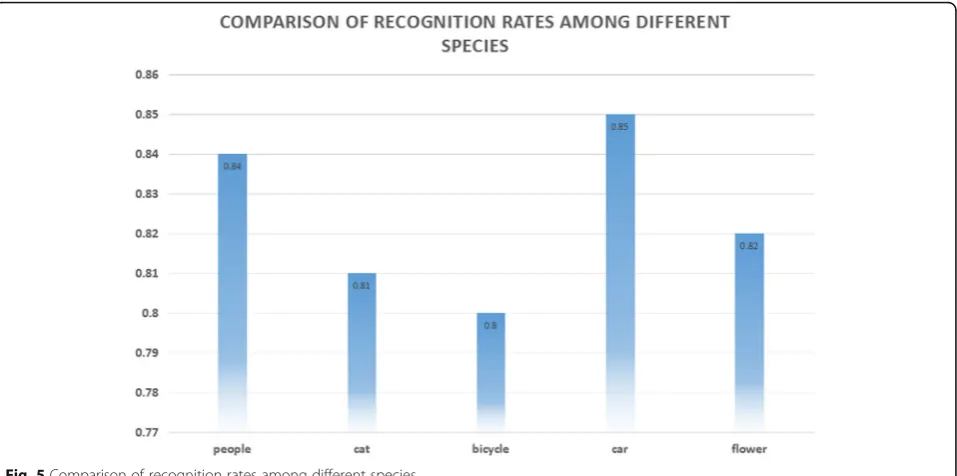
4.3 Comparison of recognition rates among different species
As can be seen from the following table, the recognition rate of this method is generally the same among differ-ent species, reaching more than 80% level, among which the accuracy of this method is relatively high in classify-ing clearly defined images such as cars. This may be due to the fact that clearly defined images have greater ad-vantages in feature extraction.
4.4 Time-consuming comparison of SVM, KNN, BP, and CNN methods
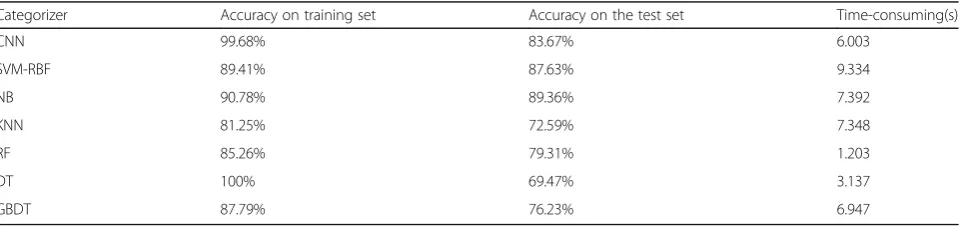
On the premise of feature extraction using the same loss function method constructed by M3CE, the selection of classifier is the key factor to affect the automatic detec-tion accuracy of human physiological funcdetec-tion. There-fore, this paper discusses the influence of different classifiers on classification accuracy in this part (Table1). The following table summarizes the influence of some common classifiers on classification accuracy. These classifiers include linear kernel support vector machine (SVM-Linear), Gao Si kernel support vector machine (SVM-RBF), and Naive Bayes (NB) (NB)k-nearest neigh-bor (KNN), random forest (RF), and decision. Strategy tree (DT) and gradient elevation decision tree (GBDT).
The experimental results show that the accuracy of CNN classifier is higher than that of other classifiers in training set and test set. Although the speed of DT is the fastest when it is used for automatic detection of hu-man physiological function in the classifier contrast ex-periment, its accuracy on the test set is only 69.47% unacceptable.由In this paper, the following conclusions can be drawn in the comparison experiment of classifier: compared with other six common classifiers, CNN has
the highest accuracy, and the spending of 6 s is accept-able in the seven classifiers of comparison.
First, because each test image needs to be compared with all the stored training images, it takes up a lot of storage space, consumes a lot of computing resources, and takes a lot of time to calculate. Because in practice, we focus on testing efficiency far higher than training ef-ficiency. In fact, the convolution neural network that we want to learn later reaches the other extreme in this trade-off: although the training takes a lot of time, once the training is completed, the classification of new test data is very fast. Such a model is in line with the actual use of the requirements.
5 Conclusions
Deep convolution neural networks are used to identify scaling, translation, and other forms of distortion-invari-ant images. In order to avoid explicit feature extraction, the convolutional network uses feature detection layer to learn from training data implicitly, and because of the weight sharing mechanism, neurons on the same feature mapping surface have the same weight. The ya training network can extract features byWparallel computation, and its parameters and computational complexity are obviously smaller than those of the traditional neural network. Its layout is closer to the actual biological neural network. Weight sharing can greatly reduce the complexity of the network structure. Especially, the multi-dimensional input vector image WDIN can effect-ively avoid the complexity of data reconstruction in the process of feature extraction and image classification. Deep convolution neural network has incomparable ad-vantages in image feature representation and classifica-tion. However, many researchers still regard the deep convolutional neural network as a black box feature ex-traction model. To explore the connection between each layer of the deep convolutional neural network and the visual nervous system of the human brain, and how to make the deep neural network incremental, as human beings do, to compensate for learning, and to increase understanding of the details of the target object, further research is needed.
Table 1Comparison before different classifiers
Categorizer Accuracy on training set Accuracy on the test set Time-consuming(s)
CNN 99.68% 83.67% 6.003
SVM-RBF 89.41% 87.63% 9.334
NB 90.78% 89.36% 7.392
KNN 81.25% 72.59% 7.348
RF 85.26% 79.31% 1.203
DT 100% 69.47% 3.137
GBDT 87.79% 76.23% 6.947
Classification Bicycle Car Bus Motor Flower
Abbreviations
Ann:Artificial neural network; BP: Backpropagation; called NB-CNN: Convolutional neural network and Naive Bayes; CNN: Convolutional neural network; MLP: Multilayer perceptron; ODI: Omnidirectional image; VFSR: Very fine spatial resolution; VR: Virtual reality
Acknowledgements
The authors thank the editor and anonymous reviewers for their helpful comments and valuable suggestions.
About the author
Xin Mingyuan was born in Heihe, Heilongjiang, P.R. China, in 1983. She received the Master degree from harbin university of science and technology, P.R. China. Now, she works in School of computer and information engineering, Heihe University, His research interests include Artificial intelligence, data mining and information security.
Wang yong was born in Suihua, Heilongjiang, P.R. China, in 1979. She received the Master degree from qiqihaer university, P.R. China. Now, she works in School of Heihe University, His research interests include Artificial intelligence, Education information management.
Funding
This work was supported by University Nursing Program for Young Scholars with Creative Talents in Heilongjiang Province (No.UNPYSCT-2017104). Scientific research items of basic research business of provincial higher education institutions of Heilongjiang Provincial Department of Education (No.2017-KYYWF-0353).
Availability of data and materials
Please contact author for data requests.
Authors’contributions
All authors take part in the discussion of the work described in this paper. XM wrote the first version of the paper. XM and WY did part experiments of the paper. XM revised the paper in a different version of the paper, respectively. All authors read and approved the final manuscript.
Competing interests
The authors declare that they have no competing interests.
Publisher’s Note
Springer Nature remains neutral with regard to jurisdictional claims in published maps and institutional affiliations.
Author details
1School of Computer and Information Engineering, Heihe University, No. 1
Xueyuan Road education science and technology zone, Heihe, Heilongjiang, China.2Heihe University, No. 1 Xueyuan Road education science and technology zone, Heihe, Heilongjiang, China.
Received: 17 October 2018 Accepted: 7 January 2019
References
1. E. Newman, M. Kilmer, L. Horesh,Image classification using local tensor singular value decompositions(IEEE, international workshop on computational advances in multi-sensor adaptive processing. IEEE, Willemstad, 2018), pp. 1–5.
2. X. Wang, C. Chen, Y. Cheng, et al, Zero-shot image classification based on deep feature extraction. United Kingdom: IEEE Transactions on Cognitive & Developmental Systems,10(2), 1–1 (2018).
3. A.A.M. Al-Saffar, H. Tao, M.A. Talab,Review of deep convolution neural network in image classification(International conference on radar, antenna, microwave, electronics, and telecommunications. IEEE, Jakarta, 2018), pp. 26–31.
4. A.B. Said, I. Jemel, R. Ejbali, et al.,A hybrid approach for image classification based on sparse coding and wavelet decomposition(Ieee/acs, international conference on computer systems and applications. IEEE, Hammamet, 2018), pp. 63–68.
5. Huang G, Chen D, Li T, et al. Multi-Scale Dense Networks for Resource Efficient Image Classification. 2018.
6. V. Gupta, A. Bhavsar, Feature importance for human epithelial (HEp-2) cell image classification. J Imaging.4(3), 46 (2018).
7. L. Yang, A.M. Maceachren, P. Mitra, et al., Visually-enabled active deep learning for (geo) text and image classification: a review. ISPRS Int. J. Geo-Inf.7(2), 65 (2018).
8. Chanti D A, Caplier A. Improving bag-of-visual-words towards effective facial expressive image classification Visigrapp, the, International Joint Conference on Computer Vision, Imaging and Computer Graphics Theory and Applications. 2018.
9. X. Long, H. Lu, Y. Peng, X. Wang, S. Feng, Image classification based on improved VLAD. Multimedia Tools Appl.75(10), 5533–5555 (2016). 10. B. Kieffer, M. Babaie, S. Kalra, et al.,Convolutional neural networks for
histopathology image classification: training vs. using pre-trained networks
(International conference on image processing theory. IEEE, Montreal, 2018), pp. 1–6.
11. J. Zhao, T. Fan, L. Lü, H. Sun, J. Wang, Adaptive intelligent single particle optimizer based image de-noising in shearlet domain. Intelligent Automation & Soft Computing23(4), 661–666 (2017).
12. Mou L, Ghamisi P, Zhu X X. Unsupervised spectral-spatial feature learning via deep residual conv-Deconv network for hyperspectral image classification IEEE transactions on geoscience & Remote Sensing. 2018,(99):1–16.
13. Newman E, Kilmer M, Horesh L. Image classification using local tensor singular value decompositions IEEE, international workshop on computational advances in multi-sensor adaptive processing. IEEE, 2018:1–5.
14. S.A. Quadri, O. Sidek, Quantification of biofilm on flooring surface using image classification technique. Neural Comput. & Applic.24(7–8), 1815– 1821 (2014).
15. X.-C. Yin, Q. Liu, H.-W. Hao, Z.-B. Wang, K. Huang, FMI image based rock structure classification using classifier combination. Neural Comput. & Applic.20(7), 955–963 (2011).
16. Z. Yan, V. Jagadeesh, D. Decoste, et al., HD-CNN: hierarchical deep convolutional neural network for image classification. Eprint Arxiv 4321-4329 (2014).
17. C. Zhang, X. Pan, H. Li, et al., A hybrid MLP-CNN classifier for very fine resolution remotely sensed image classification. Isprs Journal of Photogrammetry & Remote Sensing140, 133–144 (2018).
18. Chaib S, Yao H, Gu Y, et al. Deep feature extraction and combination for remote sensing image classification based on pre-trained CNN models. International Conference on Digital Image Processing. 2017: 104203D.
19. S. Roychowdhury, J. Ren,Non-deep CNN for multi-modal image classification and feature learning: an azure-based model(IEEE international conference on big data. IEEE, Washington, D.C., 2017), pp. 2893–2812.
20. M.Z. Afzal, A. Kölsch, S. Ahmed, et al.,Cutting the error by half: investigation of very deep CNN and advanced training strategies for document image classification(Iapr international conference on document analysis and recognition. IEEE computer Society, Kyoto, 2017), pp. 883–888.
21. X. Fu, L. Li, K. Mao, et al., inChinese High Technology Letters. Remote sensing image classification based on CNN model (2017).
22. Sachin R, Sowmya V, Govind D, et al. Dependency of various color and intensity planes on CNN based image classification. International Symposium on Signal Processing and Intelligent Recognition Systems. Springer, Cham, Manipal, 2017:167–177.
23. Shima Y. Image augmentation for object image classification based on combination of pre-trained CNN and SVM. International Conference on Informatics, Electronics and Vision & 2017, International sSymposium in Computational Medical and Health Technology. 2018:1–6.
24. J.Y. Lee, J.W. Lim, E.J. Koh, A study of image classification using HMC method applying CNN ensemble in the infrared image. Journal of Electrical Engineering & Technology13(3), 1377–1382 (2018).
25. Zhang C, Pan X, Zhang S Q, et al. A rough set decision tree based Mlp-Cnn for very high resolution remotely sensed image classification. ISPRS -International Archives of the Photogrammetry, Remote Sensing and Spatial Information Sciences, 2017:1451–1454.
26. M. Kumar, Y.H. Mao, Y.H. Wang, T.R. Qiu, C. Yang, W.P. Zhang, Fuzzy theoretic approach to signals and systems: Static systems. Inf. Sci.418, 668– 702 (2017).
28. Z. Sun, F. Li, H. Huang,Large scale image classification based on CNN and parallel SVM. International conference on neural information processing
(Springer, Cham, Manipal, 2017), pp. 545–555.