Efficient calculation of heterogeneous non-equilibrium statistics in coupled firing-rate models

S H O R T R E P O R T

Open Access

Efficient calculation of heterogeneous

non-equilibrium statistics in coupled

firing-rate models

Cheng Ly

_{, Woodrow L. Shew}

_{and Andrea K. Barreiro}

*_{Correspondence:[email protected]} 1_{Department of Statistical Sciences} and Operations Research, Virginia Commonwealth University, Richmond, USA

Full list of author information is available at the end of the article

Abstract

Understanding nervous system function requires careful study of transient

(non-equilibrium) neural response to rapidly changing, noisy input from the outside world. Such neural response results from dynamic interactions among multiple, heterogeneous brain regions. Realistic modeling of these large networks requires enormous computational resources, especially when high-dimensional parameter spaces are considered. By assuming quasi-steady-state activity, one can neglect the complex temporal dynamics; however, in many cases the quasi-steady-state assumption fails. Here, we develop a new reduction method for a general

heterogeneous firing-rate model receiving background correlated noisy inputs that accurately handles highly non-equilibrium statistics and interactions of

heterogeneous cells. Our method involves solving an efficient set of nonlinear ODEs, rather than time-consuming Monte Carlo simulations or high-dimensional PDEs, and it captures the entire set of first and second order statistics while allowing significant heterogeneity in all model parameters.

Keywords: Neural network model; Reduction method; Non-equilibrium statistics; Heterogeneity

1 Introduction

Advances in neural recording technologies have enabled experimentalists to simultane-ously measure activity across different regions with cellular resolution [1–4]. However, it is still a technical challenge to measure the many biophysical parameters that govern this multi-region activity. This challenge is exacerbated by the fact that cortical neurons are heterogeneous (i.e., parameters vary across cells) [5] and have significant trial-to-trial noise [6]. Given these features, computational modeling of neural networks often requires exploration of a high-dimensional parameter space and lengthy, time-consuming Monte Carlo simulations. Thus, efficient methods to simulate [7] or approximate network statis-tics [8] are needed. Aside from computational benefits, streamlined equations for network activity offer potential benefits for mathematical analysis.

We previously developed a fast approximation method [9] for the complete first and second order statistics of a firing-rate network model based on the Wilson–Cowan model [10], and applied it to the olfactory sensory pathway [11]. However, those methods as-sumed that the statistics of neural activity are stationary (i.e., in steady state). Many

ral systems rely on processing of time-varying, high frequency stimuli. The resulting neu-ral responses are often transient, and a quasi-steady-state (QSS) approximation fails to capture the actual response statistics. For example, in the rodent vibrissa sensory [12], auditory [13–15], and electrosensory systems [16], stimuli and responses modulate on the order of a few milliseconds, i.e., much faster than the membrane time constants of neurons. Indeed, there is evidence that coding capabilities strongly depend on the timing of stimuli [17] (e.g., in the olfactory bulb [18–20]), further necessitating accurate model-ing of varymodel-ing neural activity. Modelmodel-ing studies show the need to account for time-varying stimuli in calculating spiking statistics [21] and in capturing neural mechanisms such as divisive gain modulation [22]. Mathematical theory to efficiently characterize non-equilibrium heterogeneous spiking statistics is scarce despite the potential to shed light on crucial transient neural responses. Thus, it is clear that accurate modeling of time-varying neural activity would benefit mechanistic investigations of neural processing.

Here we present a method to approximate the non-equilibrium statistics of a general heterogeneous coupled firing-rate model of neural networks receiving background cor-related noise, in which we: (i) assume weak coupling; equivalently, that neural activity is pairwise normal, and (ii) account for the entire probability distribution of inputs. The result is a computationally fast method because it requires the user to solve coupled non-linear ODEs, rather than to simulate and average many realizations of coupled SDEs or numerically solve a high-dimensional PDE. The method performs much better than the related QSS method [9] in several representative examples; our code is freely available (see Availability of data and materials section).

2 Model equations and method

Each cell is modeled by a single activity variablexj, which may represent membrane

volt-age, calcium concentration, etc., and which evolves according to the following equation:

τj

dxj

dt = –xj+μ˜j+σ˜jηj(t) +

Nc

k=1

gjkFk

xk(t)

, j= 1, 2, . . . ,Nc (1)

(see [10]), whereFk(·)≥0 is a nonlinear function mapping input activity to firing rate or

response (often called the F-I curve). All cells receive background noiseηjuncorrelated in

time but instantaneously correlated across different cells:ηj(t)= 0,ηj(t)ηj(t)=δ(t–t),

andηj(t)ηk(t)=cjkδ(t–t) forj=kwithcjk∈(–1, 1). The parametersμ˜jandσ˜jmodel

background noisy input. The parametergjkrepresents coupling strength from the

presy-naptickth cell and is a signed quantity;gjk< 0 represents inhibitory coupling (Fig.1(A)).

We wish to compute all of the first and second order time-varying statistics:

Mean activity μj(t) :=xj(t),

Variance of activity σ_j2(t) :=x_j2(t) –μ2_j(t),

Covariance of activity Covj,k(t) :=xjxk(t) –μj(t)μk(t),

Mean firing νj(t) :=

Fj(xj)

(t),

Variance of firing Varνj(t)

:=F_j2(xj)

(t) –ν_j2(t),

Covariance of firing Cov(νj,νk;t) :=

Fj(xj)Fk(xk)

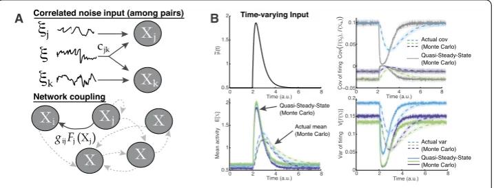
Figure 1(A) Schematic of network model. Top: Cells receive background correlated noiseξj(t) =σjηj˜ (t). Bottom: Network coupling via nonlinear function of activity that we choose to be a sigmoidal function. (B) A network ofNc= 3 coupled cells with randomly chosen parameters. With fast inputμ(t) (top-left) relative

to the time scale, the actual non-equilibrium statistics (dash curves) are very different from the

quasi-steady-state, or QSS (fixedμ(t) at timet, solid curves). Upper right shows all three pairs of covariance of firing Cov(νj,νk) for (j=k); bottom row shows the mean activityE[Xj] and variance of firing Var(νj). In all

Monte Carlo simulations here and throughout the paper, we used 1 million realizations; see Sect.2.3

Table 1 For convenience, we abbreviate the following quantities. Whenj=kin the double integrals ofM_F, the bivariate normal distributionj,kis replaced with the standard normal distribution1.

Note that order of the arguments matters inM_F:M_F(j,k)=M_F(k,j) in general. The quantities in bottom three rows depend on the statistics of the activityμ(·),σ(·)

Abbreviation Definition

1(y) √1

2πe –y2/2

j,k(y1,y2) 1

2π

1–c2 jk

exp(–1₂yT₍1 cjk cjk1)

–1_y )

Dj,k cjk

˜ σjσ˜k τjτk

E1(k) Fk(σk(t)y+μk(t))1(y)dy E2(k)

F2_k(σk(t)y+μk(t))1(y)dy

MF(j,k) Fk(σk(t)y1+μk(t))y2j,k(y1,y2)dy1dy2

where the angular brackets·denotes averaging over realizations.

2.1 Reduction of the Fokker–Planck equation

The corresponding probability density function p(x,t) of X:= (x1, . . . ,xNc), defined as

p(x,t)dx=P(X(t)∈(x,x+dx)), satisfies the Fokker–Planck equation [23]:

∂p(x,t) ∂t = –

Nc

l=1

∂ ∂xl

1 τl

–xl+μ˜l+ Nc

k=1

glkFk(xk)

p(x,t)

+1 2

j,k

Dj,k

∂2p(x,t) ∂xj∂xk

= –

Nc

l=1

∂ ∂xl

Jl(x,t) +

1 2

j,k

Dj,k

∂2_p(x,t)

∂xj∂xk

, (2)

whereDj,k=cjk˜

σjσ˜k

τjτk (see Table1), and the sum withDj,kis taken over allNc×Ncpairs of

(j,k). For convenience we have defined theprobability fluxorcurrent, asJl(x,t) :=τ1l[–xl+

˜

μl+

Nc

k=1glkFk(xk)]p(x,t) in the right-most part of Eq. (2). This high-dimensional partial

2.2 Moment closure methods

One way to tackle high-dimensional systems is through “moment closure” methods, in which state variables are integrated or averaged out, and assumptions on moments used to reduce the number of equations. Such approaches have been used in the physical [24, 25] and life sciences [26–28]; see [29] for another type of reduction method for this kind of equation. Here, we propose a closure based on weak coupling, and therefore pairwise Gaussianity in the activity variables.

Without coupling, i.e.gjk= 0, the steady-state solution of Eq. (2) is simply a multivariate

Gaussian distribution with meanμ= [μ˜1, . . . ,μ˜Nc] and covariance matrixCovj,k= cjk τj+τkσ˜jσ˜k

in the steady state. This motivates a closure of the system in which we assumeXis Gaus-sian: i.e.Xj=σj+Yjμj, whereYjis a standard normal random variable, with parameters

μjandσjto be determined. We also assume the joint marginal distributions are bivariate

Gaussian:

P(xj,xk) :=

p(x,t)dxj,k; (Xj,Xk)∼N μj μk ,

σ_j2 cjkσjσk

cjkσjσk σk2

, (3)

whereNdenotes a bivariate Gaussian distribution, anddxj,kdenotes integrating over all

Ncvariables exceptxjandxk.

Note that the integrated quantity ∂p(_∂x,t)_t dx= 0, as any probability distribution must integrate to unity. We multiply Eq. (2) byxjand integrate the equation over allNcvariables,

dx=dxjdxj(where againdxj=dx1· · ·dxj–1dxj+1· · ·dxNc):

dμj(t)

dt = –

Nc

l=1

∂ ∂xl

Jl(x,t)xjdxjdxj+

1 2

l1,l2

Dl1,l2

∂2p(x,t) ∂xl1∂xl2

xjdxjdxj, (4)

where dμj(t)

dt =

∂ ∂t

xjp(x,t)dx. Consider the first term on the RHS: whenl=j, we have

_∂

∂xlJl(x,t)xjdxjdxj=

_∂

∂xlJl(x,t)dxlxjdxjdxl,j=

Jl|xl=∞

xl=–∞xjdxjdxj=

0xjdxjdxj= 0. The

last equality comes from no flux at±∞:Jl|xl=∞

xl=–∞= 0. A similar calculation applies to the

second term, for allNc×Ncvalues of (l1,l2): whenl1=jandl2=j, first integrate inxl1and

xl2, and then use the fact that there is no density at±∞:p(x,t)| xl_1/2=∞

xl_1/2=–∞= 0; whenl1/2=j,

first integrate inxj, then integrate by parts, using∂jp(x,t)xj| xj=∞

xj=–∞= 0 and∂jp(x,t)|

xj=∞

xj=–∞= 0.

Therefore, Eq. (4) becomes

dμj(t)

dt = 1 τj

–μj(t) +μ˜j+ Nc

k=1

gjkE1(k)

, (5)

where we have used the approximationFk(xk)p(x,t)dx≈E1(k) (see Table1) by assuming

the marginalxkPDF is a normal distribution with meanμk(t) and varianceσk2(t).

To derive a similar equation for the varianceσ_j2(t), we multiply Eq. (2) byx2

j and again

integrate over all variables:

dE_j2(t)

dt = –

Nc

l=1

∂ ∂xl

Jl(x,t)x2jdxjdxj+

1 2

l1,l2

Dl1,l2

∂2p(x,t) ∂xl1∂xl2

x2_jdxjdxj, (6)

whereEj2(t) =

Following the same type of manipulations and again using the no density condition at

±∞:p(x,t)|xl1/2=∞

xl1/2=–∞= 0, we get

dEj2(t)

dt =Dj,j+ 2 τj

–Ej2(t) +μ˜_jμ_j(t) + Nc

k=1

gjk

xjFk(xk)p(x,t)dx

. (7)

We now employ our approximation,xj=μj(t) +yjσj(t) whereyjis a standard normal

ran-dom variable, to close the last term in Eq. (7). We further approximate yjFk(μk(t) +

ykσk(t))p(x,t)dxby assuming the joint marginal distribution of (xj,xk) is bivariate

nor-mal, and use the definition ofMFin Table1:yjFk(μk(t) +ykσk(t))p(x,t)dx≈MF(j,k).

Therefore, the equation for the second moment is

τj

dEj2(t)

dt =

˜

σ_j2

τj

+ 2

–E_j2(t) +μ˜_jμ_j(t) + Nc

k=1

gjk

μj(t)E1(k) +σj(t)MF(j,k)

. (8)

To derive the analogous equation for theCovj,k(t), the procedure is almost exactly the

same except that Eq. (2) is multiplied byxjxk, and two terms from the sum (over probability

fluxesJl) contribute, whenl=jandl=k. The result is

τjτk

dEj,k(t)

dt =cjkσ˜jσ˜k+τk

–Ej,k+μ˜jμk(t) +

l

gjl

μk(t)E1(l) +σk(t)MF(k,l)

+τj

–Ej,k+μ˜kμj(t) +

l

gkl

μj(t)E1(l) +σj(t)MF(j,l). (9)

Whenj=kin Eq. (9), we recover Eq. (8).

The full set of kinetic equations given by Eq. (5), (8), and (9) form a system of nonlinear coupled ODEs withNc+Nc(Nc+ 1)/2 variables. The statistics of the firing rate (i.e.νj=

Fj(xj)) are obtained from a standard change of variables.

Ifμ˜,σ˜ are constant in time, the system (Eq. (5), (8), (9)) settles to a steady state:

μj=μ˜j+ Nc

k=1

gjkE1(k), σj2= ˜

σ_j2

2τj

+σj Nc

k=1

gjkMF(j,k),

Cov_j,kτj+τk 2 =cjk

˜

σjσ˜k

2 + σj(t)

2 τj

Nc

l=1

gklMF(j,l) +

σk(t)

2 τk

Nc

l=1

gjlMF(k,l).

(10)

A common approximation to non-equilibrium statistics is to assume that the system immediately equilibrates to the steady-state solution of Eq. (1) at each time point for the time-dependent parametersμ˜j(t),σ˜j(t), which we call the QSS method. We will find that

the QSS method fails to capture meaningful features of network activity with relatively fast input.

2.3 Monte Carlo simulations

in all figures represent 1 standard deviation above and below the mean, which is ap-proximated via the sample standard deviation on 1000 samples of 1000 realizations each: S=

1 999

1000

j=1 (X(j) –X)2, whereXis the average over 1 million realizations andX(j) is

an average over 1000 realizations.

3 Results

We implement our method for networks of various sizesNc, with two time-varying

in-puts. We chooseFto be a sigmoidal:Fj(·) = 0.5(1 +tanh((x–xrev,j)/xsp,j))∈[0, 1] (arbitrary

units,xrev,j andxsp,jare parameters). To include heterogeneity, parameters were chosen

randomly from the following distributions:

τj∼N

1, 0.12, μ˜j∼U– 0.5, σ˜j∼U+ 1,

xrev,j∼N

0, 0.12, xsp,j∼0.35U+ 0.05,

(11)

where U∈[0, 1] is a uniform random variable, and N is a normal random variable. The input correlation matrix Cr was generated so to have approximately independent off-diagonal entries as follows: (i) create a matrix A with i.i.d. entries Ajk ∼N(0, 0.82);

(ii) create a diagonal matrix Λ_d

s from the vector ds where ds(j) = 1/

(AT_A)

jj; (iii) set Cr = (Λ_d

s)A

T_A(Λ

ds). By construction, Cr is symmetric positive semidefinite with 1’s

on the diagonal. Finally, the entries of the coupling matrix G are independently cho-sen: Gjk ∼N(0,vl) where vl = (l/10)2 with l= 1 for Figs. 1–2, and l = 1, 2, 3, or 4 in

Figs.3–4. All entries of G are nonzero (i.e. coupling is all-to-all), with inhibitory, exci-tatory, and self-coupling cases.

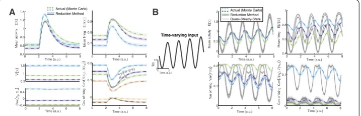
Figure1(B) shows that with relatively fast time-varyingμ(t), a network ofNc= 3 cells

has complex non-equilibrium network statistics that cannot be approximated by the QSS approximation (i.e., assuming the system immediately equilibrates to the steady-state so-lution for each time point). This is true for the complete set of activity and response statis-tics, although for brevity only a subset are shown. All parameters are chosen as in Eq. (11) except forμ(t), which is the same for all three cells.

Figure2(A) shows that the time-varying method (Eq. (5), (8), and (9)), when applied to same network as in Fig.1(B), gives accurate results for the complete set of first/second order statistics. Figure2(B) shows a detailed comparison of another instance of theNc= 3

Figure 3Applying our method to a larger network ofNc= 50 neurons. As coupling strength increases (red →green→cyan→purple), performance worsens. (A) The absolute value of the error of our method with the Monte Carlo simulations as a function of time. EachAverage Absolute Errortime point is averaged over the entire set of statistics (i.e., for the mean and variances the average is over all 50, for covariances the average is over 1225 = 49∗25). (A) Left: the average for the mean activityXj(solid) and mean firingF(Xj) =νj

(dot-dashed); with the progression of colors (red to purple) representing stronger (i.e., larger) coupling values Gj,k. (A) Middle: Error of covariances (thinner lines,j=k) and variances (thicker lines,j=k) of activityXj.

(A) Right: Error of covariances (thinner lines,j=k) and variances (thicker lines,j=k) of firingF(Xj) =νj.

(B) Representative comparisons of our method with the Monte Carlo simulations. (B) Left: although the average error increases with coupling magnitude, the discrepancies are not noticeable for mean activity and firing (not shown). (B) Middle: the method is visibly worse for the variance of activity as coupling magnitude increases. (B) Right: the method is visibly worse as coupling magnitude increases – note that the weakest coupling (red) is between green (second weakest) and purple (strongest)

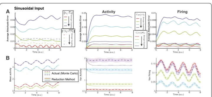
Figure 4Applying our method to a larger network ofNc= 50 neurons. Same format as Fig.3except with

sinusoidal input (see Fig.2(B)). (A) Again as coupling strength increases (red→green→cyan→purple), performance worsens. (B) Representative comparisons of our method with the Monte Carlo simulations. (B) Left: although the average error increases with coupling magnitude, the discrepancies are not noticeable for mean activity and firing (not shown). (B) Middle: the method is visibly worse for the variance of activity as coupling magnitude increases. (B) Right: the method is visibly worse as coupling magnitude increases for variance of firing – note that the weakest coupling (red) has largest variance of firing

Thus far we have only consider small networks. In Figs.3and4, our methods are applied to a large network ofNc= 50 coupled cells where the magnitude of the coupling strengths

vary: Gjk∼N(0, l 2

100), forl= 1, 2, 3, 4. Figure3shows the results with pulse input (Fig.1(B)

upper-left) applied to all 50 cells, while Fig.4shows results from applying the sinusoidal input (Fig. 2(B) left) to all 50 cells. Figure3(A) (top row) shows the error between our method and the actual (Monte Carlo) statistics; we plot the absolute error averaged over all cells or pairs:

Average Absolute Error = 1 M

M

j=1

XMC(t) –XMethod(t),

i.e., for mean and variance of activity and firing,M= 50; for covariance of activity and firing, averaging over allM= 50∗49/2 distinct pairs. All six sets of statistics are shown in Fig.3(A): the left panel shows the average absolute error for both mean activity (solid) and mean firing (dot-dashed), middle panel shows the variance (thick solid) and covariance of activity (thin solid), the right panel shows the variance (thick solid) and covariance (thin solid) of firing. In all cases, as the coupling magnitude increases (red→green→cyan

→purple), the error increases. For reference, the bottom row (Fig.3(B)) compares our method with the Monte Carlo simulations for a particular cell (or cell pair); the chosen cell or pair is the one that most closely matches the average absolute error. In Fig.3(B), we only show three out of the six statistics (left is mean activity, middle is variance of activity, right is variance of firing) because these clearly show the performance of our method in relation to the size of the average absolute error. Figure4has exactly the same format as Fig.3, but with sinusoidal input.

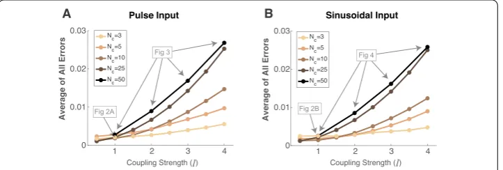
Finally, in Fig.5, to assess the performance of our method, we plot the absolute value of the error averaged over all six statistics and over all cells/pairs (vertical axis) as a func-tion of a measure of coupling strengthl(Fig.5(A) is with pulse input, (B) with sinusoidal input). Each curve shows a different network size, ranging fromNc= 3, 5, 10, 25, 50, with

a particular instance of randomly chosen parameters for each curve.a_{The magnitude of}

Figure 5Our method implicitly assumes weak coupling, so as the average magnitude of the coupling strength increases, the performance decreases. We demonstrate this with several instances of coupling matrices and network sizesNc= 3, 5, 10, 25, andNc= 50 with the four coupling values in Figs.3and4, using

the same pulse (A) and sinusoidal (B) inputs. On vertical axis, we plot the average absolute error overallfirst and second order statistics, including all cells and pairs, while on the horizontal axis, we plot a measure of average magnitude of the coupling valuesl. Note that, sinceGjk∼N(0, l

2

100), the average of all|Gjk|is l 5√2πin

the infinite limitNc→ ∞. For reference, some of the points on these curves are from prior figures, denoted in

the coupling strength,l, on the horizontal axis is from Gjk∼N(0, l 2

100), so that the average

of allN2

c values of|Gjk|is ₅√l_2π in the infinite limitNc→ ∞. Not surprisingly, the

aver-age error increases as coupling strength increases for each curve. Assessing how much absolute error is acceptable depends on the purposes of the approximation, but for refer-ence, the instances of networks from prior figures are denoted in gray. Figure5indicates that, as long as the average absolute error is below 0.01, our method likely performs very well, independent of network size (cf. with Figs.2–4). Average absolute errors larger than 0.01 might indicate at least some of the statistics calculated by our method are likely to be inaccurate, although others may be accurate depending on cell or pair (cf. Figs.3–4).

4 Conclusion

The role of mathematical theory and computation in addressing neuroscience questions is as vital as ever despite tremendous advances in recording technologies. As detailed in the Introduction, the common assumption of equilibrium neural network responses is in-accurate in many neural systems. Here we derived and implemented a reduction method to calculate the complete set of first and second ordernon-equilibriumstatistics in cou-pled heterogeneous networks of firing-rate models [10] receiving background correlated noise [30–32]. Importantly, our method captures the non-equilibrium statistics when they are vastly different from the quasi-steady-state, and works very well even with significant heterogeneity in all model parameters. As the overall magnitude of the coupling strengths increase, the performance of our method declines because the moment closure method assumes weak coupling.

Mathematical reductions that well approximate the statistics of firing-rate models [33], such as the one described here, are likely to be relevant for future theoretical studies of neural networks for several reasons. Wilson–Cowan type models [10] are commonly used because of their simplicity and history of successful application in neural systems. Analysis of spiking statistics using mean-field methods often results in similar firing-rate equations [34–37]. Finally, such methods might be useful for mechanistic investigations of neural function across multiple brain regions that commonly rely on larger models with more parameters and complexity [7,11].

Acknowledgements

We thank the Shew Lab, in particular Shree Hari Gautam, for their expertise in the olfactory system that motivated some of this work. We thank the Southern Methodist University (SMU) Center for Research Computation for providing computational resources.

Funding

CL is supported by a grant from the Simons Foundation (# 355173). These funding bodies had no role in the design of the study; collection, analysis, and interpretation of computational results; or in writing the manuscript.

Abbreviations

QSS, Quasi-Steady-State; RHS, Right-hand side; ODEs, Ordinary differential equations; PDEs, Partial differential equations; SDEs, Stochastic differential equations.

Availability of data and materials

Software used to generate the computational results shown here can be found at http://github.com/chengly70/nonequilibriumFR.

Ethics approval and consent to participate Not applicable.

Competing interests

Consent for publication Not applicable.

Authors’ contributions

CL, WLS, AKB designed the project. AKB and CL wrote the software. CL designed the figures. CL, WLS, AKB wrote the paper. All authors read and approved the final manuscript.

Author details

1_{Department of Statistical Sciences and Operations Research, Virginia Commonwealth University, Richmond, USA.} 2_{Department of Physics, University of Arkansas, Fayetteville, USA.}3_{Department of Mathematics, Southern Methodist} University, Dallas, USA.

Endnote

a _{On each curve, the intrinsic parameters are randomly chosen and fixed aslvaries. The same realization ofG}

jkis used

for each curve, and simply scaled bylto vary the coupling strength.

Publisher’s Note

Springer Nature remains neutral with regard to jurisdictional claims in published maps and institutional affiliations.

Received: 4 February 2019 Accepted: 28 April 2019 References

1. Ahrens MB, Orger MB, Robson DN, Li JM, Keller PJ. Whole-brain functional imaging at cellular resolution using light-sheet microscopy. Nat Methods. 2013;10(5):413–20.

2. Prevedel R, Yoon Y-G, Hoffmann M, Pak N, Wetzstein G, Kato S, Schrödel T, Raskar R, Zimmer M, Boyden ES, et al. Simultaneous whole-animal 3d imaging of neuronal activity using light-field microscopy. Nat Methods. 2014;11(7):727–30.

3. Kandel ER, Markram H, Matthews PM, Yuste R, Koch C. Neuroscience thinks big (and collaboratively). Nat Rev Neurosci. 2013;14(9):659–64.

4. Lemon WC, Pulver SR, Höckendorf B, McDole K, Branson K, Freeman J, Keller PJ. Whole-central nervous system functional imaging in larval drosophila. Nat Commun. 2015;6:7924.

5. Marder E. Variability, compensation, and modulation in neurons and circuits. Proc Natl Acad Sci. 2011;108:15542–8. 6. Cohen MR, Kohn A. Measuring and interpreting neuronal correlations. Nat Neurosci. 2011;14:811–9.

7. Stringer C, Pachitariu M, Steinmetz NA, Okun M, Bartho P, Harris KD, Sahani M, Lesica NA. Inhibitory control of correlated intrinsic variability in cortical networks. eLife. 2016;5:19695.

8. Gerstner W, Kistler W. 5. Spiking Neuron Models. Cambridge: Cambridge University Press; 2002. p. 147–163. 9. Barreiro A, Ly C. Practical approximation method for firing-rate models of coupled neural networks with correlated

inputs. Phys Rev E. 2017;96:022413.https://doi.org/10.1103/PhysRevE.96.022413.

10. Wilson HR, Cowan JD. Excitatory and inhibitory interactions in localized populations of model neurons. Biophys J. 1972;12:1–24.

11. Barreiro A, Gautam S, Shew W, Ly C. A theoretical framework for analyzing coupled neuronal networks: application to the olfactory system. PLoS Comput Biol. 2017;13:1005780.

12. Ritt JT, Andermann ML, Moore CI. Embodied information processing: vibrissa mechanics and texture features shape micromotions in actively sensing rats. Neuron. 2008;57:599–613.

13. Grothe B, Klump GM. Temporal processing in sensory systems. Curr Opin Neurobiol. 2000;10:467–73.

14. Köppl C. Phase locking to high frequencies in the auditory nerve and cochlear nucleus magnocellularis of the barn owl, Tyto alba. J Neurosci. 1997;17:3312–21.

15. Mason A, Oshinsky M, Hoy R. Hyperacute directional hearing in a microscale auditory system. Nature. 2001;410:686–90.

16. Benda J, Longtin A, Maler L. A synchronization–desynchronization code for natural communication signals. Neuron. 2006;52:347–58.

17. van Steveninck RRdR, Lewen GD, Strong SP, Koberle R, Bialek W. Reproducibility and variability in neural spike trains. Science. 1997;275(5307):1805–8.

18. Cury KM, Uchida N. Robust odor coding via inhalation-coupled transient activity in the mammalian olfactory bulb. Neuron. 2010;68(3):570–85.

19. Gschwend O, Beroud J, Carleton A. Encoding odorant identity by spiking packets of rate-invariant neurons in awake mice. PLoS ONE. 2012;7(1):30155.

20. Grabska-Barwi ´nska A, Barthelmé S, Beck J, Mainen ZF, Pouget A, Latham PE. A probabilistic approach to demixing odors. Nat Neurosci. 2017;20:98–106.

21. Liu CY, Nykamp DQ. A kinetic theory approach to capturing interneuronal correlation: the feed-forward case. J Comput Neurosci. 2009;26(3):339–68.

22. Ly C, Doiron B. Divisive gain modulation with dynamic stimuli in integrate-and-fire neurons. PLoS Comput Biol. 2009;5(4):1000365.https://doi.org/10.1371/journal.pcbi.1000365.

23. Risken H. 1. The Fokker–Planck equation: methods of solutions and applications. New York: Springer; 1989. 24. Chapman SI, Cowling TG. The Mathematical Theory of Non-Uniform Gases. New York: Cambridge University Press;

1970.

25. Dreyer W, Junk M, Kunik M. On the approximation of the Fokker–Planck equation by moment systems. Nonlinearity. 2001;14:881–906.

27. Williams GS, Huertas MA, Sobie EA, Jafri MS, Smith GD. Moment closure for local control models of calcium-induced calcium release in cardiac myocytes. Biophys J. 2008;95(4):1689–703.

28. Buice MA, Cowan JD, Chow CC. Systematic fluctuation expansion for neural network activity equations. Neural Comput. 2010;22:377–426.

29. Stinchcombe AR, Forger DB. An efficient method for simulation of noisy coupled multi-dimensional oscillators. J Comput Phys. 2016;321:932–46.

30. Doiron B, Litwin-Kumar A, Rosenbaum R, Ocker G, Josi´c K. The mechanics of state-dependent neural correlations. Nat Neurosci. 2016;19(3):383–93.

31. Barreiro AK, Ly C. When do correlations increase with firing rates in recurrent networks? PLoS Comput Biol. 2017;13:1005506.https://doi.org/10.1371/journal.pcbi.1005506.

32. Barreiro A, Ly C. Investigating the correlation-firing rate relationship in heterogeneous recurrent networks. J Math Neurosci. 2018;8:8.https://doi.org/10.1186/s13408-018-0063-y.

33. Bressloff PC. Path-integral methods for analyzing the effects of fluctuations in stochastic hybrid neural networks. J Math Neurosci. 2015;5:4.

34. Ermentrout B. Reduction of conductance-based models with slow synapses to neural nets. Neural Comput. 1994;6(4):679–95.

35. Faugeras O, Touboul J, Cessac B. A constructive mean-field analysis of multi-population neural networks with random synaptic weights and stochastic inputs. Front Comput Neurosci. 2009;3:1.

36. Rosenbaum R, Smith MA, Kohn A, Rubin JE, Doiron B. The spatial structure of correlated neuronal variability. Nat Neurosci. 2017;20(1):107–14.