SFB
823
Optimal designs for model
averaging in non-nested
models
Discussion Paper
Kira Alhorn, Holger Dette,
Kirsten Schorning
Optimal designs for model averaging in non-nested models
Kira Alhorn
Technische Universit¨at Dortmund Fakult¨at Statistik
44221 Dortmund, Germany
Holger Dette, Kirsten Schorning Fakult¨at f¨ur Mathematik Ruhr-Universit¨at Bochum
44799 Bochum, Germany
March 30, 2019
Abstract
In this paper we construct optimal designs for frequentist model averaging estimation. We derive the asymptotic distribution of the model averaging estimate with fixed weights in the case where the competing models are non-nested and none of these models is cor-rectly specified. A Bayesian optimal design minimizes an expectation of the asymptotic mean squared error of the model averaging estimate calculated with respect to a suit-able prior distribution. We demonstrate that Bayesian optimal designs can improve the accuracy of model averaging substantially. Moreover, the derived designs also improve the accuracy of estimation in a model selected by model selection and model averaging estimates with random weights.
Keywords: Model selection, model averaging, model uncertainty, optimal design, Bayesian optimal designs
1
Introduction
There exists an enormous amount of literature on selecting an adequate model from a set of candidate models for statistical analysis. Numerous model selection criteria have been devel-oped for this purpose. These procedures are widely used in practice and have the advantage of delivering a single model from a class of competing models, which makes them very attractive for practitioners. Exemplarily, we mention Akaike’s information criterion (AIC), the Bayesian information criterion (BIC) and its extensions, Mallow’s Cp, the generalized cross-validation
and the minimum description length (see the monographs of Burnham and Anderson (2002), Konishi and Kitagawa (2008) and Claeskens and Hjort (2008) for more details). Different crite-ria have different properties, such as consistency, efficiency and parsimony (used in the sense of
Claeskens and Hjort (2008, Chapter 4)). Overall there seems to be no universally optimal model selection criterion and different criteria might be preferable in different situations depending on the particular application.
On the other hand, there exists a well known post-selection problem in this approach because model selection introduces an additional variance that is often ignored in statistical inference after model selection (see P¨otscher (1991) for one of the first contributions discussing this issue). This post-selection problem is inter alia attributable to the fact, that estimates after model selection behave like mixtures of potential estimates. For example, ignoring the model selection step (and thus the additional variability) may lead to confidence intervals with coverage probability smaller than the nominal value, see for example Chapter 7 in Claeskens and Hjort (2008) for a mathematical treatment of this phenomenon.
An alternative to model selection is model averaging, where estimates of a target parame-ter are smoothed across several models, rather than restricting inference on a single selected model. This approach has been widely discussed in the Bayesian literature, where it is known as “Bayesian model averaging” (see the tutorial of Hoeting et al. (1999) among many others). For Bayesian model averaging prior probabilities have to be specified. This might not always be possible and therefore Hjort and Claeskens (2003) also proposed a “frequentist model av-eraging”, where smoothing across several models is commonly based on information criteria. Kapetanios et al. (2008) demonstrated that the frequentist approach is a worthwhile alternative to Bayesian model averaging. Stock and Watson (2003) observed that averaging predictions usually performs better than forecasting in a single model. Hong and Preston (2012) substanti-ate these observations with theoretical findings for Bayesian model averaging if the competing models are “sufficiently close”. Further results pointing in this direction can be found in Raftery and Zheng (2003), Schorning et al. (2016) and Buatois et al. (2018).
Independently of this discussion there exists a large amount of research how to optimally design experiments under model uncertainty (see Box and Hill (1967); Stigler (1971); Atkinson and Fedorov (1975) for early contributions). This work is motivated by the fact that an optimal design can improve the efficiency of the statistical analysis substantially if the postulated model assumptions are correct, but may be inefficient if the model is misspecified. Many authors suggested to choose the design for model discrimination such that the power of a test between competing regression models is maximized (see Ucinski and Bogacka (2005); L´opez-Fidalgo et al. (2007); Tommasi and L´opez-Fidalgo (2010) or Dette et al. (2015) for some more recent references). Other authors proposed to minimize an average of optimality criteria from different models to obtain an efficient design for all models under consideration (see Dette (1990), Zen and Tsai (2002); Tommasi (2009) among many others).
Although model selection or averaging are commonly used tools for statistical inference under model uncertainty most of the literature on designing experiments under model uncertainty does not address the specific aspects of these methods directly. Optimal designs are usually
constructed to maximize the power of a test for discriminating between competing models or to minimize a functional of the asymptotic variance of estimates in the different models. To the best of our knowledge Alhorn et al. (2019) is the first contribution, which addresses the specific challenges of designing experiments for model selection or model averaging. These authors constructed optimal designs minimizing the asymptotic mean squared error of the model averaging estimate and showed that optimal designs can yield a reduction of the mean squared error up to 45%. Moreover, they also showed that these designs improve the performance of estimates in models chosen by model selection criteria. However, their theory relies heavily on the assumption of nested models embedded in a framework of local alternatives as developed by Hjort and Claeskens (2003).
The goal of the present contribution is the construction of optimal designs for model averaging in cases where the competing models are not nested (note that in this case local alternatives cannot be formulated). Moreover, in contrast to most of the literature, we also consider the situation where all competing models mispecify the data underlying truth. In order to derive an optimality criterion, which can be used for the determination of optimal designs in this con-text, we further develop the approach of Hjort and Claeskens (2003) and derive an asymptotic theory for model averaging estimates for classes of competing models which are non-nested. Optimal designs are then constructed minimizing the asymptotic mean squared error of the model averaging estimate and it is demonstrated that these designs yield substantially more precise model averaging estimates. Moreover, these designs also improve the performance of estimates after model selection. Our work also contributes to the discussion of the superiority of model averaging over model selection. Most of the results presented in literature indicate that model averaging has some advantages over model selection in general. We demonstrate that conclusions of this type depend sensitively on the class of models under consideration. In particular we observe some advantages of estimation after model selection if the competing models are of rather different shape. Nevertheless, the optimal designs developed in this paper improve both estimation methods, where the improvement can be substantial in many cases. The remaining part of this paper is organized as follows. The pros and cons of model averaging and model selection are briefly discussed in Section 2 where we introduce the basic methodology and investigate the impact of similarity of the candidate models on the performance of the different estimates. In Section 3 we develop asymptotic theory for model averaging estimation in the case where the models are non-nested and all competing models might misspecify the underlying truth. Based on these results we derive a criterion for the determination of optimal designs. In Section 4 we study the performance of these designs by means of a simulation study. Finally, technical assumptions and proofs are given Section 6.
2
Model averaging versus model selection
In this section we introduce the basic terminology and also illustrate in a regression framework that the superiority of model averaging about estimation in a model chosen by model selection depends sensitively on the class of competing models.
2.1
Basic terminology
We consider data obtained at k different experimental conditions, say x1, . . . , xk chosen in a
design space X. At each experimental condition xi one observes ni responses, say yi1, . . . , yini
(i = 1, . . . , k), and the total sample size is n = Pk
i=1ni. We also assume that the responses
yi1, . . . , yini are realizations of random variables of the form
Yij =ηs(xi, ϑs) +εij, i= 1, . . . , k, j = 1, . . . , ni, s= 1, . . . , r, (2.1)
where the regression functionηsis a differentiable function with respect to the parameterϑsand
the random errorsεij are independent normally distributed with mean 0 and common variance
σ2. Furthermore, the index s in η
s corresponds to different models (with parameters ϑs) and
we assume that there arer competing regression functions η1, . . . , ηr under consideration.
Having r different candidate models (differing by the regression functions ηs) a classical
ap-proach for estimating a parameter of interest, say µ, is to calculate an information criterion for each model under consideration and estimate this parameter in the model optimizing this information criterion. For this purpose, we denote the density of the normal distribution corre-sponding to a regression model (2.1) byfs(· |xi, θs) with parameterθs = (σ2, ϑs)>and identify
the different models by their densitiesf1, . . . , fr(note that in the situation considered in this
sec-tions these only differ in the mean). Using the observasec-tions yn = (y11, . . . , y1n1, y21, . . . , yknk)
>
estimate we calculate in each model the maximum likelihood estimate ˆ
θn,s = arg max θs∈Θs
`n,s(θs |yn) (2.2)
of the parameter θs, where
`n,s(θs|yn) = 1 n k X i=1 ni X j=1 logfs(yij |xi, θs) (2.3)
is the log-likelihood in candidate model fs (s = 1, . . . r). Note that we do not assume that
estimate ˆθn,s of the parameter θs yields an estimate
ˆ
µs =µs(ˆθn,s), (2.4)
for the quantity of interest, whereµs is the target parameter in model s.
For example, regression models of the type (2.1) are frequently used in dose finding studies (see MacDougall (2006) or Bretz et al. (2008)). In this case a typical target function µs of interest
is the “quantile” defined by
µs(θs) = inf x∈ X ηs(x, ϑs)−ηs(a, ϑs) ηs(b, ϑs)−ηs(a, ϑs) ≥α . (2.5)
The value defined in (2.5) is well-known as EDα, that is, the effective dose at which 100×α%
of the maximum effect in the design spaceX = [a, b] is achieved.
We now briefly discuss the principle of model selection and averaging to estimate the target parameter µ. For model selection we choose the model fs∗ from f1, . . . , fs, which maximizes
Akaike’s information criterion (AIC)
AIC(fs |Yn) = 2`n,s(ˆθn,s |yn)−2ps, (2.6)
whereps is the number of parameters in modelfs (see Claeskens and Hjort (2008), Chapter 2).
The target parameter is finally estimated by ˆµ= µs∗(ˆθn,s∗). Obviously, other model selection
schemes, such as the Bayesian or focussed information criterion can be used here as well, but we restrict ourselves to the AIC for the sake of a transparent presentation.
Roughly speaking, model averaging is a weighted average of the individual estimates in the competing models. It might be viewed from a Bayesian (see for example Wassermann (2000)) or a frequentist point of view (see for example Claeskens and Hjort (2008)) resulting in differ-ent choices of model averaging weights. We will focus here on non-Bayesian methods. More explicitly, assigning nonnegative weights w1, . . . , wr to the candidate models f1, . . . , fr, with
Pr
i=1wi = 1, the model averaging estimate for µis given by
ˆ µmav = r X s=1 wsµs(ˆθn,s). (2.7)
Frequently used weights are uniform weights (see, for example Stock and Watson (2004), Kapetanios et al. (2008)). More elaborate model averaging weights can be chosen depend-ing on the data. For example, Claeskens and Hjort (2008) define smooth AIC-weights as
wsmAICs (Yn) = exp{1 2AIC(fs |Yn)} Pr s=1exp{ 1 2AIC(fs|Yn)} . (2.8)
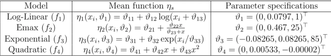
Model Mean function ηs Parameter specifications Log-Linear (f1) η1(xi, ϑ1) =ϑ11+ϑ12log(xi+ϑ13) ϑ1 = (0,0.0797,1)> Emax (f2) η2(xi, ϑ2) =ϑ21+ϑϑ22x 23+x ϑ2 = (0,0.467,25) > Exponential (f3) η3(xi, ϑ3) =ϑ31+ϑ32exp(xi/ϑ33) ϑ3 = (−0.08265,0.08265,85)> Quadratic (f4) η4(xi, ϑ4) = ϑ41+ϑ42x+ϑ43x2 ϑ4 = (0,0.00533,−0.00002)>
Table 1: Models and parameters used for the simulation study.
Alternative data dependent weights can be constructed using other information criteria or model selection criteria. There also exists a vast amount of literature on determining optimal data dependent weights such that the resulting mean squared error of the model averaging estimate is minimal (see Hjort and Claeskens (2003), Hansen (2007) or Liang et al. (2011) among many others). For the sake of brevity we concentrate on smooth AIC-weights here, but similar observations as presented in this paper can also be made for other data dependent weights.
2.2
The class of competing models matters
In this section we illustrate the influence of the candidate set on the properties of model averaging estimation and estimation after model selection by means of a brief simulation study. For this purpose we consider four regression models of the form (2.1), which are commonly used in dose-response modeling and specified in Table 1 with corresponding parameters. Here we adapt the setting of Pinheiro et al. (2006) who model the dose-response relationship of an anti-anxiety drug, where the dose of the drug may vary in the interval X = [0,150]. In particular, we have k = 6 different dose levels xi ∈ {0,10,25,50,100,150} and patients are allocated to
each dose level most equally, where the total sample size isn∈ {50,100,250}. We consider the problem of estimating the ED0.4, as defined in (2.5).
To investigate the particular differences between both estimation methods we choose two dif-ferent sets of competing models from Table 1. The first set
S1 ={f1, f2, f4} (2.9)
contains the log-linear, the Emax and the quadratic model, while the second set
S2 ={f1, f2, f3} (2.10)
contains the log-linear, the Emax and the exponential model. The setS1 serves as a prototype
set of “similar” models while the set S2 contains models of more “different” shape. This is
illustrated in Figure 1. In the left panel we show the quadratic model f4 (for the parameters
0 50 100 150 0.0 0.1 0.2 0.3 0.4 Dose Response η4 η1 η2 0 50 100 150 0.0 0.1 0.2 0.3 0.4 Dose Response η3 η1 η2
Figure 1: Left panel: quadratic model (solid line) and its best approximations by the log-linear (dashed line) and the Emax model (dotted line) with respect to the Kullback-Leibler divergence
(2.11). Right panel: exponential model (solid line) and its best approximations by the log-linear (dashed line) and the Emax model (dotted line).
and an Emax model (f2) with respect to the Kullback-Leibler divergence
1 6 6 X i=1 Z f4(y|xi, θ4) log f4(y|xi, θ4) fs(y|xi, θs) dy , s= 1,2. (2.11)
In this case, all models have a very similar shape and we obtain for the ED0.4 the values 32.581,
32.261 and 33.810 for the log-linear (f1), Emax (f2) and quadratic model (f4). Similarly the
right panel shows the exponential model (f3, solid line) and its corresponding best
approxima-tions by the log-linear model (f1) and the Emax model (f2). Here we observe larger differences
between the models in the candidate set and we obtain for the ED0.4 the values 58.116, 42.857
and 91.547 for the modelsf1, f2 and f3, respectively.
All results presented in this paper are based on 1000 simulations runs generating in each run n observations of the form
yij(l) =ηs(xi, ϑs) +ε (l)
ij, i= 1, . . . , k, j = 1, . . . , ni, (2.12)
where the errors ε(l)ij are independent centered normal distributed random variables with σ2 =
0.1 andηs is one of the modelsη1, . . . , η4(with parameters specified in Table 1). The parameter
µ = ED0.4 is estimated by model averaging with uniform, smooth AIC weights in (2.8) and
estimation after model selection by the AIC criterion.
In Table 2 and 3 we show the simulated mean squared errors of the model averaging estimates with uniform weights (left column), smooth AIC-weights (2.8) (middle column) and estimation after model selection (right column). Here, different rows correspond to different models. The numbers printed in bold face indicate the estimation method with the smallest mean squared error.
model sample size uniform weights smooth AIC-weights model selection n = 50 437.045 498.323 758.978 f1 n= 100 223.291 218.99 285.062 n= 250 111.973 82.713 78.371 n = 50 286.638 329.904 515.32 f2 n= 100 189.785 203.796 251.836 n= 250 62.792 64.854 66.54 n = 50 276.037 361.101 669.873 f4 n= 100 190.662 244.558 391.443 n= 250 92.653 109.852 139.859 n = 50 1503.903 1372.31 1381.033 f3 n= 100 1109.622 856.484 729.912 n= 250 864.163 398.144 255.604
Table 2: Simulated mean squared error of different estimates of the ED0.4. The set of candidate models isS1 ={f1, f2, f4}. Left column: model averaging with uniform weights; middle column: model averaging with smooth AIC-weights; right column: estimation after model selection.
2.2.1 Models of similar shape
We will first discuss the results for the set of similar models in (2.9) (see Table 2). If the data generating model is an element of the set of candidate models, model averaging with uniform weights performs very well. Model averaging with smooth AIC-weights yields an about 10% -25% larger mean squared error (except for two cases, where it performs better than model averaging with uniform weights). On the other hand the mean squared error of estimation after model selection is substantially larger than that of model averaging, if the sample size is small. This is a consequence of the additional variability associated with data-dependent weights. For example, if the sample size is n = 50 and the data generating model is given by f1, the mean squared errors of the model averaging estimates with uniform and smooth
AIC-weights and the estimate after model selection are given by 437.0, 498.3 and 759.0, respectively. The corresponding variances are given by 235.2, 337.6 and 599.7, respectively. For the squared bias the order is exactly the opposite, that is 201.9, 160.7, 159.3, but the differences are not so large. This means that the bias can be reduced by using random weights, because these put more weight on the “correct” model. As a consequence, compared to model averaging with uniform weights the performance of model averaging with smooth AIC-weights and the estimate after model selection improves with increasing sample size. Nevertheless, if the “true” model is an element of the candidate set and the functions in this set have a similar shape, model averaging performs better than estimation after model selection. In particular, model averaging with (fixed) uniform weights yield very reasonable results. These observation coincide with the findings of Schorning et al. (2016) and Buatois et al. (2018) who compared model averaging and model selection in the context of dose finding studies (see also Chen et al. (2018) for similar
estimation method
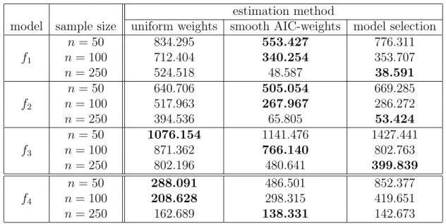
model sample size uniform weights smooth AIC-weights model selection n = 50 834.295 553.427 776.311 f1 n= 100 712.404 340.254 353.707 n= 250 524.518 48.587 38.591 n = 50 640.706 505.054 669.285 f2 n= 100 517.963 267.967 286.272 n= 250 394.536 65.805 53.424 n = 50 1076.154 1141.476 1427.441 f3 n= 100 871.362 766.140 802.763 n= 250 802.196 480.641 399.839 n = 50 288.091 486.501 852.377 f4 n= 100 208.628 298.315 419.651 n= 250 162.689 138.331 142.673
Table 3: Simulated mean squared error of different estimates of the ED0.4. The set of candidate models isS2 ={f1, f2, f3}. Left column: model averaging with uniform weights; middle column: model averaging with smooth AIC-weights; right column: estimation after model selection.
results for the AIC in the context of ordered probit and nested logit models).
The situation changes if none of the candidate models from the set S1 is the “true” model.
This is illustrated in the lower part of Table 2, where we show results if the exponential model f3 is used for generating the data. We observe that model averaging with uniform weights
is outperformed by model averaging with smooth AIC-weights. Moreover, the estimate after model selection is even better, if the sample size increases. These observations can be explained by the different shapes of the regression functions, as illustrated in Figure 1. By a suitable choice of parameters the quadratic model can adapt to the shape of the exponential model, whereas the log-linear and the Emax model still have different forms (see right panel of Figure 1 for the best approximations that are possible using the log-linear and the Emax model). Thus, incorporating these models in a model averaging estimate yields a large bias, that can be reduced substantially by data dependent weights or by model selection. For example, if n = 100 the squared bias of the model averaging estimate with uniform weights is 981.631, whereas the model averaging estimate with smooth AIC-weights and the estimate after model selection show a squared bias of 328.634 and 69.465, respectively.
2.2.2 Models of more different shape
We will now consider the candidate setS2 in (2.10), which serves as an example of more different
models and includes the log-linear, the Emax and the exponential model. The simulated mean squared errors of the three estimates of the ED0.4 are given in Table 3. The upper part of the
for model selection and averaging. In contrast to Section 2.2.1 we observe only one scenario, where model averaging with uniform weights gives the smallest mean squared error (but in this case model averaging with smooth AIC-weights yields very similar results). If the sample size increases model averaging with smooth AIC-weights and estimation after model selection yield a substantially smaller mean squared error. An explanation of this observation consists in the fact that for a candidate set containing models with a rather different shape model averaging with uniform weights produces a large bias. On the other hand model averaging with smooth AIC-weights and estimation after model selection adapt to the data and put more weight on the “true” model, in particular if the sample size is large. As estimation after model selection has a larger variance and the variance is decreasing with increasing sample size, the bias is dominating the mean squared error for large sample sizes and thus estimation in the model selected by the AIC is more efficient for large sample sizes.
Finally, if the data is generated according to the quadratic modelf4 6∈ S2 model averaging with
uniform weights has the smallest mean squared error if the sample is n = 50 and n = 100. In this case estimation in the model selected by the AIC performs much worse (due to its large variance). However, the differences become smaller with increasing sample size. In particular for n = 250 model averaging with smooth AIC-weights and estimation after model selection show a substantially better performance than model averaging with uniform weights.
The numerical study in Section 2.2.1 and 2.2.2 can be summarized as follows. The results observed in the literature have to be partially relativized. The superiority of model averaging with uniform weights can only be observed for classes of “similar” competing models and a not too large signal to noise ratio. On the other hand if the models in the candidate set are of rather different structure, model averaging with data dependent weights (such as smooth AIC-weights) or estimation after model selection may show a better performance. For these reasons we will investigate optimal/efficient designs for all three estimation methods in the following sections. We will demonstrate that a careful design of experiments can improve the accuracy of these estimates substantially.
3
Asymptotic properties and optimal design
In this section we will derive the asymptotic properties of model averaging estimates with fixed weights in the case where the competing models are not nested. The results can be used for (at least) two purposes. On the one hand they provide some understanding of the empirical findings in Section 2, where we observed, that for increasing sample size the mean squared error of model averaging estimates is dominated by its bias. On the other hand, we will use these results to develop an asymptotic representation of the mean squared error of the model averaging estimate, which can be used in the construction of optimal designs.
3.1
Model averaging for non-nested models
Hjort and Claeskens (2003) provide an asymptotic distribution of frequentist model averaging estimates making use of local alternatives which require the true data generating process to lie inside a wide parametric model. All candidate models are sub-models of this wide model and the deviations in the parameters are restricted to be of ordern−1/2. Using this assumption results in convenient approximations for the mean squared error as variance and bias are both of order O(1/n). However, in the discussion of this paper Raftery and Zheng (2003) pose the question if the framework of local alternatives is realistic. More importantly, frequentist model averaging is also often used for non-nested models (see for example Verrier et al. (2014)). In this section we will develop asymptotic theory for model averaging estimation in non-nested models. In particular, we do not assume that the “true” model is among the candidate models used in the model averaging estimate.
As we will apply our results for the construction of efficient designs for model averaging estima-tion we use the common notaestima-tion of this field. To be precise, letY denote a response variable and letxdenote a vector of explanatory variables defined on a given compact design space X. Suppose that Y has a density g(y | x) with respect to a dominating measure. For estimating a quantity of interest, say µ, from the distribution g we use r different parametric candidate models with densities
f1(y |x, θ1), . . . , fr(y|x, θr) (3.1)
whereθsdenotes the parameter in thesth model, which varies in a compact parameter space, say
Θs ⊂Rps (s = 1, ..., r). Note, that in general we do not assume that the density g is contained
in the set of candidate models in (3.1) and that the regression model (2.1) investigated in Section 2 is a special case of this general notation.
We assume thatk different experimental conditions, say x1, . . . , xk, can be chosen in a design
spaceX and that at each experimental conditionxione can observeniresponses, sayyi1, . . . , yini
(thus the total sample size is n = Pk
i=1ni), which are realizations of independent identically
distributed random variablesYi1, . . . , Yini with densityg(· |xi). For example, ifgcoincides with
fs then the density of the random variables Yi1, . . . , Yini is given by fs(· |xi, θs) (i= 1, . . . , k).
To measure efficiency and to compare different experimental designs we will use asymptotic arguments and consider the case limn→∞ nni = ξi ∈ (0,1) for i = 1, . . . , k. As common in
optimal design theory we collect this information in the form
ξ ={x1, . . . , xk;ξ1, . . . , ξk}, (3.2)
which is called approximate design in the following discussion (see, for example, Kiefer (1974)). For an approximate design ξ of the form (3.2) and total sample size n a rounding procedure is applied to obtain integersni taken at each xi (i= 1, . . . , k) from the not necessarily integer
The asymptotic properties of the maximum likelihood estimate (calculated under the assump-tion that fs is the correct density) is derived under certain assumptions of regularity (see the
Assumptions (A1)-(A6) in Section 6). In particular, we assume that the functionsfs are twice
continuously differentiable with respect toθs and that several expectations of derivatives of the
log-densities exist. For a given approximate design ξ and a candidate density fs we denote by
KL(g :fs|θs, ξ) = Z g(y|x) log g(y |x) fs(y|x, θs) dydξ(x), (3.3)
the Kullback-Leibler divergence between the models g and fs and assume that
θ∗s,g(ξ) = arg min
θs∈Θs
KL(g :fs|θs, ξ) (3.4)
is unique for eachs∈ {1, . . . , r}. For notational simplicity we will omit the dependency of the minimum on the densityg, whenever it is clear from the context and denote the minimizer by θ∗s(ξ). We also assume that the matrices
As(θs, ξ) = k X i=1 ξi Eg(·|xi) ∂2logfs(Yij |xi, θs) ∂θs∂θs> ps s,t=1 , (3.5) Bst(θs, θt, ξ) = k X i=1 ξi Eg(·|xi) ∂logfs(Yij |xi, θs) ∂θs ∂logft(Yij |xi, θt) ∂θt >ps,pt s,t=1 , (3.6)
exist, where expectations are taken with respect to the true distribution g(· |xi).
Under standard assumptions White (1982) shows the existence of a measurable maximum likelihood estimate ˆθn,s for all candidate models which is strongly consistent for the (unique)
minimizerθ∗s(ξ) in (3.4). Moreover, the estimate is also asymptotically normal distributed, that is √ n(ˆθn,s−θs∗(ξ)) D −→ N 0, A−s1(θs∗(ξ))Bss(θ∗s(ξ), θ ∗ s(ξ))A −1 s (θ ∗ s(ξ)) , (3.7)
where we assume the existence of the inverse matrices,−→D denotes convergence in distribution and we use the notations
As(θ∗s(ξ)) =As(θ∗s(ξ), ξ), Bst(θ∗s(ξ), θ
∗
t(ξ)) = Bst(θs∗(ξ), θ
∗
t(ξ), ξ) (3.8)
(s, t = 1, . . . r). The following result gives the asymptotic distribution of model averaging estimates of the form (2.7).
estimate (2.7) satisfies √ nµˆmav− r X s=1 wsµs(θ∗s(ξ)) D −→ N 0, σw2(θ∗(ξ)) , (3.9)
where the asymptotic variance is given by
σw2(θ∗(ξ)) = r X s,t=1 wswt ∂µs(θ∗ s(ξ)) ∂θs > A−s1(θs∗(ξ))Bst(θ∗s(ξ), θ ∗ t(ξ))A −1 t (θ ∗ t(ξ)) ∂µt(θ∗t(ξ)) ∂θt . (3.10) Theorem 3.1 shows, that the model averaging estimate is biased for the true target parameter µtrue, unless we have
Pr
s=1wsµs(θ∗s(ξ)) =µtrue. Hence we aim to minimize the asymptotic mean
squared error of the model averaging estimate. Note, that the bias does not depend on the sample size, while the variance is of order O(1/n).
3.2
Optimal designs for model averaging of non-nested models
Alhorn et al. (2019) determined optimal designs for model averaging minimizing the asymptotic mean squared error of the estimate calculated in a class of nested models under local alternatives and demonstrated that optimal designs lead to substantially more precise model averaging estimates than commonly used designs in dose finding studies. With the results of Section 3.1 we can develop a more general concept of design of experiments for model averaging estimation, which is applicable for non-nested models and in situations, where the “true” model is not contained in the set of candidate models used for model averaging.
To be precise, we consider the criterion
Φmav(ξ, g) = 1 nσ 2 w(θ ∗ (ξ)) + r X s=1 wsµs(θ∗s(ξ))−µtrue 2 ≈MSE(ˆµmav), (3.11)
whereµtrue is the target parameter in the “true” model with density g and σ2w(θ∗(ξ)) andθ∗s(ξ)
are defined in (3.10) and (3.4), respectively. Note that this criterion depends on the “true” distribution viaµtrue and the best approximating parameters θ∗s(ξ) =θ
∗
s,g(ξ).
For estimating the target parameter µ via a model averaging estimate of the form (2.7) most precisely a “good” designξ yields small values of the criterion function Φmav(ξ, g). Therefore,
for a given finite set of candidate models f1, . . . , fr and weights ws, s = 1, . . . , r, a design
ξ∗ is called locally optimal design for model averaging estimation of the parameter µ, if it minimizes the function Φmav(ξ, g) in (3.11) in the class of all approximate designs on X. Here
the term “locally” refers to the seminal paper of Chernoff (1953) on optimal designs for nonlinear regression models, because the optimality criterion still depends the unkown density g(y|x).
A general approach to address this uncertainty problem is a Bayesian approach based on a class of models for the density g. To be precise, let G denote a finite set of potential densities and letπ denote a probability distribution on G, then we call a design Bayesian optimal design for model averaging estimation of the parameter µif it minimizes the function
Φπmav(ξ) =
Z
G
Φmav(ξ, g)dπ(g) . (3.12)
In general, the setGcan be constructed independently of the set of candidate models. However, if there is not much prior information available one can construct a class of potential models
G from the candidate set as follows. We denote the candidate set of models in (3.1) by S. Each of these models depends on a unknown parameter θs and we denote by Ffs ⊂ Θs a
set of possible parameter values for the model fs. Now let π2 denote a prior distribution on S and for each fs ∈ S let π1(· | fs) denote a prior distribution on Ffs. Finally, we define
G={(g, θ) :g ∈ S, θ ∈ Fg}and a prior
dπ(g, θ) = dπ1(θ|g) dπ2(g), (3.13)
then the criterion (3.12) can be rewritten as
Φπmav(ξ) = Z S Z Fg Φmav(ξ, g)dπ1(θ|g)dπ2(g), (3.14)
In the finite sample study of the following section the setS and the setFg (for anyg ∈ S) are
finite, which results in a finite set G.
We conclude noting that the optimality criteria proposed in this section have been derived for model averaging estimates with fixed weights. The asymptotic theory presented here cannot be easily adapted to estimates using data-dependent (random) weights (as considered in Section 2), because it is difficult to get an explicit expression for the asymptotic distribution, which is not normal in general. Nevertheless, we will demonstrate in the following section that designs minimizing the mean squared error of model averaging estimates with fixed weights will also yield a substantial improvement in model averaging estimation with smooth AIC-weights and in estimation after model selection.
4
Bayesian optimal designs for model averaging
We will demonstrate by means of a simulation study that the performance of all considered estimates can be improved substantially by the choice of an appropriate design. For this purpose we consider the same situation as in Section 2, that is regression models of the from (2.1) with centred normal distributed errors. We also consider the two different candidate sets S1 and
S2 defined in (2.9) (log-linear, Emax and quadratic model) and (2.10) (log-linear, Emax and
exponential model), respectively.
Using the criterion introduced in Section 3 we now determine a Bayesian optimal design for model averaging estimation of the ED0.4 with uniform weights from n= 100 observations. We
require a prior distribution for the unknown density g, and we use a distribution of the form (3.13) for this purpose. To be precise, letfs(y|x, θs) denote the density of a normal distribution
with mean ηs(x, ϑs) and variance σs2 = 0.1 (s = 1, . . . , r), where the mean functions are given
in Table 1. As the criterion (3.14) does not depend on the interceptϑs1, these are not varied
and taken from Table 1. For each of the other parameters we use three different values: the values specified in Table 1 and a 10% larger and smaller value of this parameter.
Ff1 ={(0, ϑ12, ϑ13) :ϑ12= 0.0797±10%, ϑ13= 1±10%}, (4.1)
Ff2 ={(0, ϑ22, ϑ23) :ϑ22= 0.467±10%, ϑ23= 25±10%},
Ff3 ={(−0.08265, ϑ32, ϑ33) :ϑ32 = 0.08265±10%, ϑ33 = 85±10%},
Ff4 ={(0, ϑ42, ϑ43) :ϑ42= 0.00533±10%, ϑ43=−0.00002±10%}.
4.1
Models of similar shape
We will first consider the candidate setS1 ={f1, f2, f4} consisting of the log-linear, the Emax
and the quadratic model. For the definition of the prior distribution (3.13) in the criterion (3.14) we consider a uniform distributionπ2 on the setS1 and a uniform priorπ1(· |fs) on each
set Ffs in (4.1) (s = 1,2,4). The Bayesian optimal design for model averaging estimation of
the ED0.4 minimizing the criterion (3.14) has been calculated numerically using the COBYLA
algorithm (see Powell (1994)) and is given by
ξS∗
1 ={0,14.447,49.283,150; 0.227,0.167,0.365,0.240} . (4.2)
We will compare this design with the design
ξ1 ={0,10,25,50,100,150; 1/6,1/6,1/6,1/6,1/6,1/6}, (4.3)
proposed in Pinheiro et al. (2006) for a a similar setting (this design has also been used in Section 2) and the locally optimal design for estimation of the ED0.4 in the log-linear model f1
with parameterθ1 = (0,0.0797,1)> given by
ξ2 ={0,4.051,150; 0.339,0.5,0.161} (4.4)
(see Dette et al. (2010)). Results for the locally optimal designs for the estimation of the ED0.4
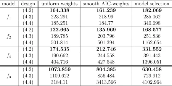
model design uniform weights smooth AIC-weights model selection (4.2) 164.338 161.239 182.069 f1 (4.3) 223.291 218.99 285.062 (4.4) 185.251 184.77 340.698 (4.2) 122.665 135.969 168.577 f2 (4.3) 189.785 203.796 251.836 (4.4) 501.814 501.394 1162.654 (4.2) 174.535 212.746 331.552 f4 (4.3) 190.662 244.558 391.443 (4.4) 404.716 427.548 1396.051 (4.2) 1073.859 804.385 630.458 f3 (4.3) 1109.622 856.484 729.912 (4.4) 3184.11 3413.566 4102.964
Table 4: Simulated mean squared errors of different estimates of the ED0.4 for different experi-mental designs. The set of candidate models is S1 ={f1, f2, f4}. Left column: model averaging estimate with uniform weights; middle column: model averaging estimate with smooth AIC-weights; right column: estimate after model selection.
same setup as in Section 2. For the sake of brevity we only report results for the sample size n= 100. Other results are available from the authors.
The corresponding results are given in Table 4, where we use the modelsf1, f2, f3 and f4 from
Table 1 to generate the data (note that the modelf3 is not in the candidate set used for model
averaging and model selection). The different columns represent the different estimation meth-ods (left column: model averaging with uniform weights; middle column: smooth AIC-weights, right column: model selection). The numbers printed in boldface indicate the minimal mean squared error for each estimation method obtained from the different experimental designs. First, we consider the situation, where the data generating model is contained in the set of candidate models S1 = {f1, f2, f4} corresponding to the upper part of the table. We observe
that in this case model averaging yields better results than estimation after model selection and this superiority is independent of the design under consideration. Compared to the designs ξ1 and ξ2 the Bayesian optimal design ξS∗1 for model averaging with uniform weights improves
the efficiency of all estimation techniques. For example, when data is generated using the log-linear model f1 the mean squared error of the model averaging estimate with uniform weights
is reduced by 26.4% and 11.3%, when the optimal design is used instead of the designs ξ1 or
ξ2, respectively. This improvement is remarkable as the design ξ2 is locally optimal for
esti-mating the ED0.4 in the model f1 and data is generated from this model. In other cases the
improvement is even more visible. For example, if data is generated by the model f2 the
im-provement in model averaging estimation with uniform weights is 35.4% and 75.6% compared to the designs ξ1 and ξ2. Moreover, although the designs are constructed for model averaging
with uniform weights they also yield substantially more accurate model averaging estimates with smooth AIC-weights and a more precise estimate after model selection. For example, if the data is generated from modelf1 the mean squared error is reduced by 26.4% and by 12.7%
for estimation with smooth AIC-weights and by 36.1% and 46.6% for estimation after model selection, respectively. Similar results can be observed for the models f2 and f4.
Next, we consider the case where the data is generated from the exponential model f3, which
is not contained in the candidate set S1. The efficiency of all three estimates improves
sub-stantially by the use of the Bayesian optimal design ξS∗1. Interestingly, the improvement is less pronounced for model averaging with uniform weights (3.2% and 66.3% compared to the designsξ1 andξ2, respectively) than for smooth AIC-weights (6.1% and 76.4%) and estimation
after model selection (13.6% and 84.6%).
Summarizing, our numerical results show that the Bayesian optimal design for model averaging estimation of the ED0.4yields a substantial improvement of the mean squared error of the model
averaging estimate with uniform weights (3.2%-75.6%), smooth AIC-weights (6.1%-76.4%) and the estimate after model selection (13.6%-85.5%) for all four models under consideration.
4.2
Models of different shape
We will now consider the second candidate set S2 consisting of the log-linear (f1) the Emax
(f2) and the exponential model (f3). For the definition of the prior distribution (3.13) in the
criterion (3.14) we use a uniform distribution π2 on the set S2 and a uniform prior π1(· | fs)
on each set Ffs (s = 1,2,3) in (4.1). For this choice the Bayesian optimal design for model
averaging estimation of the ED0.4 is given by
ξS∗2 ={0,5.529,74.303,77.186,150; 0.179,0.142,0.274,0.162,0.243}, (4.5) and has (in comparison to the design ξS∗
1 in Section 4.2) five instead of four support points.
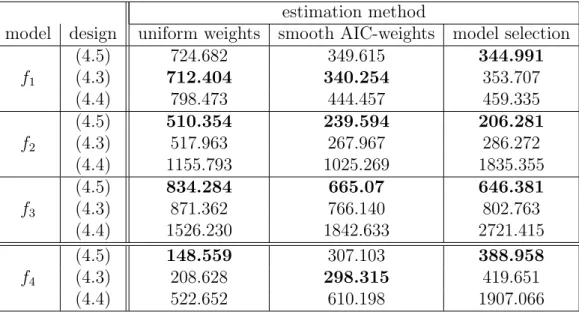
The simulated mean squared errors of the three estimates under different designs are given in Table 5. We observe again that compared to the designs ξ1 and ξ2 the Bayesian optimal
design ξS∗2 improves most estimation techniques substantially. However, if model averaging with uniform weights is used and data is generated by modelf1, the mean squared error of the
model averaging estimate from the optimal design is 1.7% larger than the mean squared error obtained by the design ξ1. For model averaging with smooth AIC-weights this difference is
2.8%. Overall, the reported results demonstrate a substantial improvement in efficiency by the use of the Bayesian optimal design independently of the estimation method. If the Bayesian optimal design is used, estimation after model selection yields the smallest mean squared error if the data is generated from a model of the candidate set S2. On the other hand, if data is
generated from modelf4 6∈ S2 model averaging with equal weights shows the best performance.
estimation method
model design uniform weights smooth AIC-weights model selection (4.5) 724.682 349.615 344.991 f1 (4.3) 712.404 340.254 353.707 (4.4) 798.473 444.457 459.335 (4.5) 510.354 239.594 206.281 f2 (4.3) 517.963 267.967 286.272 (4.4) 1155.793 1025.269 1835.355 (4.5) 834.284 665.07 646.381 f3 (4.3) 871.362 766.140 802.763 (4.4) 1526.230 1842.633 2721.415 (4.5) 148.559 307.103 388.958 f4 (4.3) 208.628 298.315 419.651 (4.4) 522.652 610.198 1907.066
Table 5: Simulated mean squared errors of different estimates of the ED0.4 for different experi-mental designs. The set of candidate models is S2 ={f1, f2, f3}. Left column: model averaging estimate with uniform weights; middle column: model averaging estimate with smooth AIC-weights; right column: estimate after model selection.
reduces the mean squared error of model averaging estimates with uniform weights up to 71.6%. Furthermore, for smooth AIC-weights and estimation after model selection the reduction can be even larger and is up to 76.6% and 88.8%, respectively. These improvements hold also for the quadratic modelf4, which is not contained in the candidate setS2 used in the definition of
the optimality criterion.
5
Conclusions
In this paper we derived the asymptotic distribution of the frequentist model averaging estimate with fixed weights from a class of not necessarily nested models. We neither assume that this class contains the “true” model. We use these results to determine Bayesian optimal designs for model averaging, which improve the estimation accuracy of the estimate substantially. Although these designs are constructed for model averaging with fixed weights, they also yield a substantial improvement of accuracy for model averaging with data dependent weights and for estimation after model selection.
We also demonstrate that the superiority of model averaging against estimation after model selection depends sensitively on the class of competing models, which is used in the model averaging procedure. If the competing models are similar (which means that a given model from the class can be well approximated by all other models), then model averaging should be preferred. Otherwise, we observe advantages for estimation after model selection, in particular,
if the signal to noise ratio is small.
Although, the new designs show a very good performance for estimation after model selection and for model averaging with data dependent weights, it is of interest to develop optimal designs, which address the specific issues of data dependent weights in the estimates. This is a very challenging problem for future research as there is no simple expression of the asymptotic mean squared error of these estimates. A first approach to solve this problem is an adaptive one and a further interesting and very challenging question of future research is to improve the accuracy of adaptive designs.
AcknowledgementsThis work has also been supported in part by the Collaborative Research Center “Statistical modeling of nonlinear dynamic processes” (SFB 823, Teilprojekt C2, T1) of the German Research Foundation (DFG).
References
Alhorn, K., Schorning, K., and Dette, H. (2019). Optimal designs for frequentist model averaging.
Biometrika, to appear.
Atkinson, A. C. and Fedorov, V. V. (1975). The design of experiments for discriminating between two rival models. Biometrika, 62:57–70.
Box, G. E. P. and Hill, W. J. (1967). Discrimination among mechanistic models. Technometrics, 9(1):57–71.
Bretz, F., Hsu, J., and Pinheiro, J. (2008). Dose finding – a challenge in statistics. Biometrical Journal, 50(4):480–504.
Buatois, S., Ueckert, S., Frey, N., Retout, S., and Mentr´e, F. (2018). Comparison of model averaging and model selection in dose finding trials analyzed by nonlinear mixed effect models. The AAPS journal, 20:56.
Burnham, K. P. and Anderson, D. R. (2002). Model Selection and Multimodel Inference: A Practical Information-Theoretic Approach (2nd ed.). Springer-Verlag, New York.
Chen, L., Wan, A. T. K., Tso, G., and Zhang, X. (2018). A model averaging approach for the ordered probit and nested logit models with applications. Journal of Applied Statistics, 45(16):3012–3052. Chernoff, H. (1953). Locally optimal designs for estimating parameters. Annals of Mathematical
Statistics, 24:586–602.
Claeskens, G. and Hjort, N. L. (2008). Model Selection and Model Averaging. Cambridge Series in Statistical and Probabilistic Mathematics. Cambridge University Press.
Dette, H. (1990). A generalization ofD- andD1-optimal designs in polynomial regression.The Annals
of Statistics, 18:1784–1805.
Dette, H., Kiss, C., Bevanda, M., and Bretz, F. (2010). Optimal designs for the emax, log-linear and exponential models. Biometrika, 97(2):513–518.
Dette, H., Melas, V. B., and Guchenko, R. (2015). Bayesiant-optimal discriminating designs. The Annals of Statistics, 43(5):1959–1985.
Hansen, B. E. (2007). Least squares model averaging. Econometrica, 75(4):1175–1189.
Hjort, N. L. and Claeskens, G. (2003). Frequentist Model Average Estimators.Journal of the American Statistical Association, 98(464):879–899.
Hoeting, J. A., Madigan, D., Raftery, A. E., and Volinsky, C. T. (1999). Bayesian model averaging: a tutorial (with comments by m. clyde, david draper and e. i. george, and a rejoinder by the authors).
Statist. Sci., 14(4):382–417.
Hong, H. and Preston, B. (2012). Bayesian averaging, prediction and nonnested model selection. Jour-nal of Econometrics, 167(2):358 – 369. Fourth Symposium on Econometric Theory and Applications (SETA).
Kapetanios, G., Labhard, V., and Price, S. (2008). Forecasting using bayesian and information-theoretic model averaging. Journal of Business & Economic Statistics, 26(1):33–41.
Kiefer, J. (1974). General Equivalence Theory for Optimum Designs (Approximate Theory). The Annals of Statistics, 2(5):849–879.
Konishi, S. and Kitagawa, G. (2008). Information Criteria and Statistical Modeling. John Wiley & Sons, New York.
Liang, H., Zou, G., Wan, A. T. K., and Zhang, X. (2011). Optimal Weight Choice for Frequentist Model Average Estimators. Journal of the American Statistical Association, 106(495):1053–1066. L´opez-Fidalgo, J., Tommasi, C., and Trandafir, P. C. (2007). An optimal experimental design criterion
for discriminating between non-normal models. Journal of the Royal Statistical Society, Series B, 69:231–242.
MacDougall, J. (2006). Analysis of Dose-Response Studies -Emax Model. In Ting, N., editor,Dose
Finding in Drug Development, pages 127–145. Springer, New York.
Pinheiro, J., Bornkamp, B., and Bretz, F. (2006). Design and analysis of dose-finding studies combining multiple comparisons and modeling procedures. Journal of Biopharmaceutical Statistics, 16:639– 656.
P¨otscher, B. M. (1991). Effects of model selection on inference. Econometric Theory, 7(2):163–185. Powell, M. J. D. (1994). A direct search optimization method that models the objective and constraint
functions by linear interpolation. In Hennart, J.-P. and Gomez, S., editors,Advances in Optimization and Numerical Analysis, pages 51–67. Dordrecht.
Pukelsheim, F. (2006). Optimal Design of Experiments. Classics in Applied Mathematics. Society for Industrial and Applied Mathematics. DOI: 10.1137/1.9780898719109.
Raftery, A. and Zheng, Y. (2003). Discussion: Performance of bayesian model averaging. Journal of the American Statistical Association, 98:931–938.
Schorning, K., Bornkamp, B., Bretz, F., and Dette, H. (2016). Model selection versus model averaging in dose finding studies. Statistics in Medicine, 35(22):4021–4040.
Stigler, S. (1971). Optimal experimental design for polynomial regression. Journal of the American Statistical Association, 66:311–318.
Journal of Economic Literature, 41(3):788–829.
Stock, J. H. and Watson, M. W. (2004). Combination forecasts of output growth in a seven-country data set. Journal of Forecasting, 23(6):405–430.
Tommasi, C. (2009). Optimal designs for both model discrimination and parameter estimation.Journal of Statistical Planning and Inference, 139:4123–4132.
Tommasi, C. and L´opez-Fidalgo, J. (2010). Bayesian optimum designs for discriminating between models with any distribution. Computational Statistics & Data Analysis, 54(1):143–150.
Ucinski, D. and Bogacka, B. (2005).T-optimum designs for discrimination between two multiresponse dynamic models. Journal of the Royal Statistical Society, Series B, 67:3–18.
van der Vaart, A. W. (1998). Asymptotic Statistics. Cambridge Series in Statistical and Probabilistic Mathematics. Cambridge University Press, Cambridge.
Verrier, D., Sivapregassam, S., and Solente, A.-C. (2014). Dose-finding studies, mcp–mod, model selection, and model averaging: Two applications in the real world. Clinical Trials, 11:476–484. Wassermann, L. (2000). Bayesian model selection and model averaging. Journal of Mathematical
Psychology, 44:92–107.
White, H. (1982). Maximum likelihood estimation of misspecified models. Econometrica, 50(1):1–25. Zen, M.-M. and Tsai, M.-H. (2002). Some criterion-robust optimal designs for the dual problem of model discrimination and parameter estimation. Sankhya: The Indian Journal of Statistics, 64:322–338.
6
Technical assumptions and proof of Theorem 3.1
6.1
Assumptions
Following White (1982) we assume:
(A1) The random variables Yij, i = 1, . . . , k, j = 1, . . . , ni are independent. Furthermore,
Yi1, . . . , Yini have a common distribution function with a measurable density g(· | xi)
with respect to a dominating measure ν.
(A2) The distribution function of each candidate models ∈ {1, . . . , r}has a measurable density fs(· |x, θs) with respect to ν (for all θs ∈Θs) that is continuous in θs.
(A3) For all x ∈ X the expectation E(log(g(Y | x))) exists (where expectation is taken with respect to g( · | x)) and for each candidate model the function y 7→ |logfs(y | x, θs)| is
dominated by a function that is integrable with respect to g(· |x) and does not depend on θs. Furthermore the Kullback-Leibler divergence (3.3) has a unique minimum
θs,g∗ (ξ) = arg min
θs∈Θs
and θ∗s,g(ξ) is an interior point of Θs.
(A4) For all x∈ X the function y7→ ∂logfs(y|x,θs)
∂θs is a measurable function for all θs ∈ Θs and
continuously differentiable with respect to θs for all y∈R.
(A5) The entries of the (matrix valued) functions
y 7→C(s)(y) = ∂ 2logf s(y|x, θs) ∂θs∂θs> , y7→D(st)(y) = ∂logfs(y|x, θs) ∂θs ∂logft(y|x, θt) ∂θt >
are dominated by integrable functions with respect to g(· |x) for all x∈ X andθs∈Θs.
(A6) The matrices Bss(θ∗s(ξ), θ∗s(ξ), ξ) and As(θs∗(ξ), ξ) in (3.5) and (3.6) are nonsingular.
(A7) The functions θs 7→µs(θs) are once continuously differentiable.
6.2
Proof of Theorem 3.1
By equation (A.2) in White (1982) we have
√ n(ˆθn,s−θ∗s(ξ)) +A −1 s (θ ∗ s(ξ)) 1 √ n k X i=1 ni X j=1 ∂logfs(Yij |xi, θ∗s(ξ)) ∂θs p −→0, (A.2)
where −→p denotes convergence in probability (note that the matrix As(θs∗) = As(θs∗, ξ) is
nonsingular by assumption). An application of the multivariate central limit theorem now leads to 1 √ n Pk i=1 Pni j=1 ∂logf1(Yij|xi,θ∗1(ξ)) ∂θ1 .. . Pk i=1 Pni j=1 ∂logfr(Yij|xi,θ∗r(ξ)) ∂θr D −→ N 0, B11 . . . B1r .. . . .. ... Br1 . . . Brr , (A.3)
where Bst =Bst(θ∗s(ξ), θ∗t(ξ), ξ) is defined in (3.6). Combining (A.2) and (A.3) we obtain the
weak convergence of the vector ˆθn= (ˆθ>n,1, . . . ,θˆ>n,r)>, that is √
n(ˆθn−θ∗(ξ))
D
−→ N(0,Σ), (A.4)
where Σ = (Σst)s,t=1,...,r is a block matrix withps×pt entries
Σst =A−s1(θ ∗ s(ξ))Bst(θs∗(ξ), θ ∗ t(ξ))A −1 t (θ ∗ t(ξ)), s, t= 1, . . . , r (A.5)
and the vector θ∗s(ξ) is given by
θ∗(ξ) = ((θ1∗(ξ))T, . . . ,(θr∗(ξ))T)T. (A.6)
Next, we define for the parameter vector θ> = (θ1>, ..., θr>) ∈ RPrs=1ps the projection π
s by
πsθ :=θs and the vector
˜ µ(θ) = µ1(π1θ), . . . , µr(πrθ) T (A.7) with derivative µ0θ = ∂µ1(θ1) ∂θ1 > 0 . . . 0 0 ∂µ2(θ2) ∂θ2 > 0 . . . 0 0 . . . 0 ∂µr(θr) ∂θr > . (A.8)
An application of the Delta method (see for example van der Vaart (1998, Chapter 3)) now shows that √ n(˜µ(ˆθn)−µ˜(θ∗(ξ))) D −→ N0, µ0θ∗(ξ)Σ µ0θ∗(ξ) > . (A.9)
The assertion finally follows from the continuous mapping theorem observing the representation
ˆ