https://doi.org/10.5194/ms-8-235-2017
© Author(s) 2017. This work is distributed under the Creative Commons Attribution 3.0 License.
Inverse dynamics and trajectory tracking control of a new
six degrees of freedom spatial 3-RPRS
parallel manipulator
Santhakumar Mohan1and Burkhard Corves2
1Discipline of Mechanical Engineering, Indian Institute of Technology, Indore, 453552, India 2Department of Mechanism Theory and Dynamics of Machines, RWTH Aachen University,
Aachen, 52072, Germany
Correspondence to:Santhakumar Mohan ([email protected])
Received: 25 April 2017 – Accepted: 9 July – Published: 28 July 2017
Abstract. This paper presents the complete dynamic model of a new six degrees of freedom (DOF) spatial 3-RPRS parallel manipulator. The geometry parameters of the manipulator are optimized for a given constant orientation workspace. Further, a robust task-space trajectory tracking control is also designed for the manipula-tor along with a nonlinear disturbance observer. To demonstrate the efficacy and show the complete performance of the proposed controller, virtual prototype experiments are executed using one of the multibody dynamics software namely MSC Adams. The computer-based virtual prototype experiment results show that the manipu-lator tracking performance is satisfactory with the proposed control scheme. In addition, the controller parameter sensitivity and robustness analyses are also accomplished.
1 Introduction
Parallel manipulators or parallel kinematic machines (PKMs) have fascinated a lot of research considerations in the past few decades for their greater performance over their serial complements, in terms of load-carrying capability, rigidity and accuracy (Merlet, 2000). Over the last few years, several parallel manipulators have matured from laboratory mod-els to marketable devices. Unquestionably, the most success-ful manipulator is the Stewart-Gough platform manipulator. However, this manipulator has an extremely complex kine-matics and coupled dynamics, and its design for a definite application remains a challenge for the researchers. There-fore, several manipulators varying in their number of degrees of freedom (DOF) from three to higher numbers (even redun-dant manipulators) have been proposed in the literature (Das-gupta and Mruthyunjaya, 2000; Merlet, 2000). Abundant 6-DOF parallel robot configurations have been proposed in the literature (Merlet, 2000). While kinematically, the number of possible configurations is limited, the number of methods for applying them is fundamentally unbounded. In addition, dis-tinct arrangements of the joints and legs may lead to very
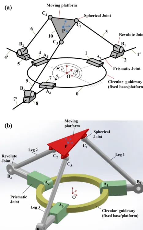
Figure 1.(a)Kinematic arrangement.(b)Solid (3-D) model of the manipulator. Conceptual design of the proposed manipulator.
a lower overall stiffness since only three kinematic chains support the mobile platform.
In this direction, a new 6-DOF spatial 3-RPRS parallel ma-nipulator was introduced in Venkatesan et al. (2014). The manipulator has three legs mounted on a circular guide at the base, which allows it to exhibit large (i.e., kinemati-cally unbounded) yaw motions, which is not very common in platform-type spatial parallel manipulators. In Venkatesan et al. (2014), only the inverse kinematic analysis of the ma-nipulator was presented. The forward kinematic problem of the same manipulator was introduced in Nag et al. (2017), wherein the solution procedure was elaborated using a nu-merical example. In the present paper, the inverse dynamic model and trajectory tracking control of the 3-RPRS ma-nipulator is studied comprehensively. The main advantage of the 3-RPRS manipulator is with respect to their dynam-ics and simplified kinematdynam-ics. As the actuators being usu-ally the heavy part of a manipulator are fixed at the base,
the mobile part of the robot is reduced to the three legs and the mobile platform. Consequently, higher velocities and ac-celerations of the mobile platform can be achieved. Another benefit is that the legs are made of only thin rods, thus, reducing the risk of leg interference. Further, the geomet-rical/physical parameters of the manipulator are also opti-mized for a given constant orientation workspace. The in-verse dynamic model is obtained using the Lagrangian dy-namic formulation method (Abdellatif and Heimann, 2009). The proposed robust task-space trajectory tracking controller is based on a centralized proportional-integral-derivative (PID) control along with a nonlinear disturbance observer. The control schemes for parallel manipulator may be prin-cipally separated into two types, joint-space control estab-lished in joint-space coordinates (Davliakos and Papadopou-los, 2008; Honegger et al., 2000; Kim et al., 2000; Nguyen et al., 1992; Yang et al., 2010), and task-space control designed based on the task-space coordinates (Kim et al., 2005; Ting et al., 2004; Wu and Gu, 2005). The joint-space control ap-proach can be readily employed as an assemblage of several independent single-input single-output (SISO) control sys-tems using the data on each actuator feedback only. A classi-cal PID control in joint-space along with gravity compensa-tion has been employed in industry, but it does not always as-sure a great performance for parallel manipulators. However, the proposed robust task-space control approach improves the overall control performance by rejecting the uncertainty and nonlinear effects in motion equations. The rejections of system or model uncertainty, unknown external disturbance and nonlinear effects in the system motions have been com-pleted in the proposed control scheme with the help of an equivalent control law; a feed-forward control scheme and a nonlinear disturbance observer along with the nonlinear PID control scheme. In the proposed task-space control method, the desired motion of the end effector in task-space is used directly as the reference input of the control scheme. That is, the motion of the end effector can be obtained from the sys-tem sensors and compared with the reference input to form a feedback error in task-space. Therefore, an exact kinemat-ics model is not required in the task-space control, and thus this method is sensitive to joint-space errors or end effector pose errors due to joint clearances and other mechanical in-accuracies. The validity of the proposed control scheme is demonstrated with the help of virtual prototype experiments. The performance of the proposed control scheme including closed-loop stability, precision, sensitivity and robustness is analysed in theory and simulation.
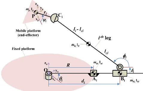
Figure 2.Kinematic arrangement ofith leg of the proposed manip-ulator.
of the proposed control scheme and the robustness analysis. Finally, the conclusions are drawn.
2 System description and mathematical background
The proposed manipulator consists of three legs or kinematic chains and each with a rotary-prismatic-rotary-spherical (RPRS) configuration as shown in Fig. 1. The base of the platform (fixed) has a circular guide on which three sliders glide, all are actuated by rotary joints at the centre of the base platform. The active prismatic joint is situated on each guide-way connecting the central rotary joint and the slider on the circular guide rail and on actuation, the prismatic joints move radially. There is a passive link which is connected with the slider block on the prismatic joint through a revolute joint and with the end-effector (mobile platform) through the help of a spherical joint. In all three legs, the starting rotary joint and the prismatic joint are actuated and other joints namely rotary and spherical joints are passive. The geometry of the manipulator is identical to the one reported in Venkatesan et al. (2014).
The kinematic arrangement along with the centre of mass locations of theith leg of the proposed manipulator is pre-sented in Fig. 2. For the purpose of kinematic analysis, a first coordinate system O(xo, yo,zo) is fixed to the fixed base
platform and a second coordinate systemP(xp,yp,zp) is
at-tached to the moving base platform (end-effector) as shown in Figs. 1 and 2. The transformation from the moving plat-form to the fixed base can be described using the position vector POP and the rotation matrixOPRof the moving plat-form with respect to the fixed base platplat-form, and are given as:
POP = Px Py Pz
T (1)
O
PR= (2)
cosαcosβ cosαsinβsinγ−sinαcosγ cosαsinβcosγ+sinαsinγ
sinαcosβ sinαsinβsinγ+cosαcosγ sinαsinβcosγ−cosαsinγ
−sinβ cosβsinγ cosβcosγ
where, Px, Py andPz are the positions of the end-effector
and α, β and γ are the roll, pitch and yaw angles of the end-effector with respect to the fixed base platform co-ordinate system. The end-effector positions and orienta-tions are considered as the task-space displacement vari-ables and the task-space displacement vector is denoted as: µ=
Px Py Pz α β γ
T
.
The vector of actuator coordinates (joint-space placements) namely rotation angles and translation dis-placements of the manipulator are denoted as: q=
θ1 θ2 θ3 d1 d2 d3T.
The position coordinates of the spherical joints on the mo-bile platform with respect to the fixed coordinate system Ci = Cxi Cyi Czi
T
can be derived as follows:
COi =Ci=PORCPi +POP (3)
where,CP
i is the position vector of theith spherical joint with
respect to the mobile coordinate systemP(xp,yp,zp) and this
vector depends on the distanceri and an angleψi (fixed
ge-ometry variables of the manipulator).iis the corresponding leg number andi=1, 2, 3. These spherical joint position co-ordinatesCican be used to establish the joint-space variables
namelyθi anddi, as follows:
θi=atan 2 Cyi, Cxi (4)
di=
q
li2−(Czi−δi)2+
q
Cxi2 +Cyi2 (5)
Further, using Eqs. (4) and (5), the position coordinates of the pointsAi andBi representing circular and linear slider
block locations can be obtained as follows:
Ai= Rcosθi Rsinθi 0 T
(6)
Bi= dicosθi disinθi 0T (7)
The forward kinematic model of this manipulator can be ob-tained with the help of loop-closure equations and forward kinematic univariate (Nag et al., 2017). The inverse kine-matic solutions of the proposed manipulator are similar to the reported one in Venkatesan et al. (2014).
The velocity and acceleration relations of the manipulator can be obtained with the help of the inverse Jacobian matrix, as given:
˙
q=J(µ)µ˙ (8) ¨
q=J(µ)µ¨+ ˙J(µ)µ˙ (9)
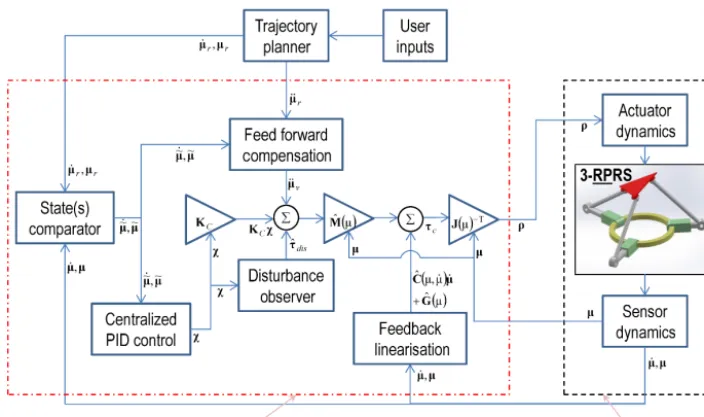
Figure 3.Block diagram representation of the proposed robust task-space control scheme.
the vector of joint-space accelerations,µ¨ ∈ <6×1is the vec-tor of task-space accelerations andJ˙(µ)∈ <6×6 is the time derivative of the inverse Jacobian matrix of the manipulator.
Understanding the manipulator dynamics and, the rela-tionship between the joint forces/moments and their effect on the joint parameters are essential in designing the sys-tem as it communicates the effect of the driving efforts on the end effector. The method adopted for the formulation of the dynamic model is Euler-Lagrange (second kind) formu-lation which is based on the total energy of the system and adopted because of its simplicity. Since the proposed system is considered as a rigid body system, the total energy of the system is only the sum of kinetic and potential energies of the individual moving components of the system. The kine-matic arrangement of the mechanism along with locations of the center of masses of bodies is presented in Fig. 2. The proposed manipulator consists of eleven bodies including the fixed platform. Each leg has three moving masses/bodies and the end-effector (refer Fig. 1). The kinetic energy and po-tential energy of the manipulator corresponds to the sum of kinetic energies and sum of potential energies of these indi-vidual moving components of the manipulator, respectively, which are given as follows:
KE=1 2
10
X
j=1
mj
˙
xcm2 j+ ˙ycm2 j+ ˙z2cmj
+Ijω2j
(10)
PE= 10
X
j=1
mjgzj (11)
where, KE and PE are the total sum of the kinetic and poten-tial energy of the mechanism.mjandIjare the
correspond-ing mass and inertia matrix of thejth link/body, respectively.
Similarly,xcmj,ycmj andzcmj are the locations of the
cen-ter of mass of thejth link/body, respectively.ωj is the
vec-tor of angular velocities of thejth link/body,x˙cmj,y˙cmj and
˙
zcmj are the linear velocities of the centre of mass of thejth
link/body, respectively.gis the gravity constant.
The Lagrange equation as per the formulation is given by
Lmechanism=KE−PE (12)
τi=
d
dt ∂L
mechanism
∂µ˙i
−∂Lmechanism
∂µi
(13)
whereLmechanismis the Lagrangian of the mechanism andτi
is the corresponding task-space force/torque which includes the control inputs and all other non-conservative external ef-fects.µi andµ˙i are the corresponding task-space
displace-ment and velocity, respectively.
The dynamic equations of motion of the proposed mecha-nism in task-space are obtained with the help of above rela-tions, and they can be represented in matrix form as follows:
M(µ)µ¨+C(µ,µ˙)µ˙+g(µ)=τ (14)
where µ¨ ∈ <6×1 is the vector of task-space accelerations. M(µ)∈ <6×6 is the inertia matrix;C(µ,µ˙)∈ <6×6 is the centripetal and Coriolis force matrix; g(µ)∈ <6×1 is the gravitational force vector; τ∈ <6×1 is the input vector. Since, the input vector consists of control inputs and other non-conservative effects, the equation of motion can be rewritten by considering the non-conservatives effects as fol-lows:
M(µ)µ¨+C(µ,µ˙)µ˙+f(µ,µ˙)+g(µ)=τc+τd (15)
Table 1.Optimized geometrical design parameters of the manipulator
Given work Geometrical design
volume parameters of the manipulator
Work xaxis yaxis zaxis End-effector Link length Maximum limit
volume limits limits limits size (s) of the linear actuators
Vw xmin xmax ymin ymax zmin zmax ri li di(max)
0.008 m3 −0.1 m 0.1 m −0.1 m 0.1 m 0.05 m 0.25 m 0.098 m 0.277 m 0.559 m
0.027 m3 −0.15 m 0.15 m −0.15 m 0.15 m 0.05 m 0.35 m 0.081 m 0.382 m 0.699 m
0.064 m3 −0.20 m 0.20 m −0.20 m 0.20 m 0.05 m 0.45 m 0.064 m 0.514 m 0.884 m
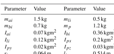
Table 2.Physical parameters of the proposed manipulator
Parameter Value Parameter Value
mai 1.5 kg mli 0.5 kg
mbi 0.7 kg mp 1.2 kg
Iai 0.07 kgm2 Ibi 0.36 kgm2
Ili 0.12 kgm2 Ipx 0.2 kgm2
Ipy 0.02 kgm2 Ipz 0.03 kgm2
ri 0.064 m li 0.514 m
<6×1is the disturbance vector in task-space (which includes external disturbances and internal uncertainties namely pa-rameter variations, noises, etc.). The actual disturbance vec-tor (τd) can be expressed as follows:
τd=τed−(1M(µ)µ¨ +1C(µ,µ˙)µ˙+1g(µ)) (16) +ζ+τum
1M(µ)=M(µ)− ˆM(µ), 1C(µ,µ˙)=C(µ,µ˙) (17)
− ˆC(µ,µ˙), 1g(µ)=g(µ)− ˆg(µ)
whereτed∈ <6×1is the vector of unknown external distur-bances in task-space; ζ∈ <6×1is the vector of process and measurement noises in task-space; τum∈ <6×1 is the vec-tor of un-modelled dynamic effects in task-space; Mˆ (µ),
ˆ
C(µ,µ˙) andgˆ(µ) are the known (inaccurate) values of the inertia matrix, centripetal and Coriolis force matrix and grav-ity vector, respectively.
Since the model is obtained in the task-space the control inputs in the joint-space can be expressed as follows:
ρ=J(µ)−Tτc (18)
where,ρ∈ <6×1is the vector of inputs (control inputs) in the joint-space;J(µ)−T ∈ <6×6is the transpose of the inverse Ja-cobian matrix of the manipulator. The obtained mathematical model that describes the dynamic behavior of the proposed manipulator is verified using a multi-body dynamics package namely MSC Adams.
Table 3. Controller parameters for the virtual prototype experi-ments.
Parameter Value Parameter Value
K 10I6×6 3 2I6×6
0 10I6×6 10 0.1 s
KP 100I6×6 KD 20I6×6
3 Robust task-space trajectory tracking control scheme
In this section, a robust nonlinear controller along with a dis-turbance observer is proposed to track a given desired task-space position (end-effector pose) trajectory of the manipu-lator. The proposed task-space control vector is given as fol-lows:
τc= ˆM(µ)µ¨v+Kξ+ ˆτdis+ ˆC(µ,µ˙)µ˙+ ˆg(µ) (19) ¨
µv= ¨µr+23˙
e
µ+32eµ
ξ= ˙
e
µ+23eµ+32R e
µdt
ˆ η=0R
ξdt
η=τd−f(µ,µ˙) ˙
e
µ= ˙µr− ˙µ
e
µ=µr−µ
(20)
where, K∈ <6×6 and0∈ <6×6 are the controller and ob-server gain matrices of the proposed controller, respectively and chosen as symmetric positive definite (SPD) matrices.
¨
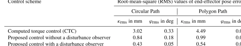
Table 4.Performance comparison of the controllers
Control scheme Root-mean-square (RMS) values of end-effector pose errors
Circular Path Polygon Path
κrmsin mm ϕrmsin deg κrmsin mm ϕrmsin deg
Computed torque control (CTC) 3.02 0.33 4.49 0.04
Proposed control without a disturbance observer 0.84 0.18 0.99 0.02
Proposed control with a disturbance observer 0.43 0.05 0.54 0.01
Figure 3 shows the block diagram representation of the proposed task-space trajectory tracking control scheme. As depicted in this figure, the block diagram flow starts with the desired task-space variables as a user input which is a function of time, t. The trajectory planner provides the desired task-space coordinates namely time trajectories of the task-space position, velocity, and acceleration vectors re-spectively, based on the user inputs. The sensor and actuator dynamics are also incorporated into the manipulator dynami-cal model. The state comparator gives the task-space tracking errors which act as an input to the proposed controller. The proposed control law can be mainly divided into four parts according to different functions. The first term is the feed-forward dynamics compensation computed by inverting plant model, is responsible for reducing and eliminating tracking errors. The second term is the centralized PID control law which acts as a feedback part results in holding the stability of the whole system. The third term of the proposed con-trol law is the disturbance estimation term based on the ob-server update law. This estimator estimates all the uncertain-ties including external disturbances and unknown nonlinear dynamics of the manipulator based on the perturbation from the dynamics of the PID controller. Therefore at each instant, the control input compensates for the uncertainty that exists during task-space trajectory tracking of the manipulator sys-tem. Finally, the feedback linearization of the nonlinear terms in the manipulator dynamics based on the known (inaccurate) values as a fourth term. Since manipulator actuators are ac-tuated in the joint-space, the control vector is transformed to the joint space with the help of inverse Jacobian matrix trans-pose. The stability analysis of the proposed control law has been derived by the Lyapunov’s direct method and explained in the following subsection.
3.1 Stability analysis
In this subsection, the Lyapunov’s direct method is employed to show the asymptotic convergence nature of the proposed controller. The following assumptions are considered to en-sure the asymptotic convergence of both disturbance estima-tion errors and tracking errors of the proposed close-loop sys-tem.
Assumption 1:The controller and estimator gain
ma-trices namelyK,0 and3are constant symmetric and positive definite matrices, by design, that is:
K=KT >0,0=0T >0,and3=3T >0 (21)
Assumption 2: The rate of change of the disturbance
acting on the manipulator is negligible in comparison with the estimated error dynamics, i.e., disturbances are slowly varying, η˙≈0 and this assumption is not overly restrictive and is commonly made in the robot manipulator literature (Kelly et al., 2005). Moreover, the lumped disturbance vectorηis assumed to be bounded and there exists a constantηU such that, 0≤ |η| ≤ηU. But this value of upper bound is not required to be known for the controller design.
Theorem 1: Consider the equations of motion of the
manipulator as given in Eq. (14), if the control input vector is chosen as defined in Eq. (18), then the task-space tracking errors and observer errors converge to zero asymptotically.
Proof 1: Consider a positive Lyapunov’s candidate
function as:
V =1
2ξ
Tξ+1
2eη
T0−1
eη (22)
where,eηis the vector of the lumped disturbance estima-tion errors and is defined as follows:
eη=η− ˆη (23)
Differentiating Eq. (21) with respect to time along with its state trajectories resulting into,
˙
V =ξTξ˙+
eη
T0−1˙
Figure 4.Block diagram representation of the proposed robust task-space control scheme.
where, ξ˙ andeη˙ are the time derivatives of the central-ized PID control vector and disturbance estimation er-rors, respectively, and these can be denoted as follows:
˙ ξ = ¨
eµ+23
˙
e
µ+32eµ= ¨µr− ¨µ+23eµ˙+32eµ (25)
˙
eη= ˙η− ˙ˆη= ˙η−0ξ (26)
From the assumption 2, it is assumed that the lumped disturbance variations are bounded and slowly varying, i.e., η˙≈0, therefore, and substituting the time deriva-tive of the centralized PID vector from Eq. (24), the manipulator equations of motion from Eq. (14), the pro-posed control vector from Eq. (18) and other relations from Eq. (19), into the Eq. (23) and simplifying, it be-comes,
˙
V = −ξTKξ (27)
Since, the controller and observer gain matricesKand 0 are constant symmetric and positive definite
matri-ces, by design. It can be observed from Eqs. (21) and (26) that the Lyapunov’s candidate function is positive definite and its time derivative is negative semidefinite in the entire state space. In order to prove the asymptoti-cally convergence of the errors to zero, let consider a set , and it contains of all points whereV˙ =0, as follows:
=nζ∈ <6×1| ˙V =0o (28)
asymptotically. i.e.,
limt→∞ξ(t)=0,limt→∞eη(t)=0, (29)
limt→∞eµ(˙ t)=0,limt→∞eµ(t)=0.
Therefore the manipulator follows the given desired task-space trajectory with minimal errors.
Remark 1:If the lumped disturbance term is fast vary-ing, i.e.,η˙6=0 then a sufficient condition for the Lya-punov function derivativeV˙ in Eq. (26) to be negative semi-definite, is given as
˙
V = −ξTKξ +
eη
T0−1η˙ (30)
eη
T0−1η˙ ≥0 (31)
where,0is the observer gain matrix and it is a constant symmetric and positive definite matrix by design, and by proper choice of this matrix can always satisfy the negative definite condition. In worst condition, value of
eη
T0−1η˙>0 is a small positive scalar. Then the Lya-punov function is a non-negative constant, such that
V(t)→last→ ∞. Furthermore,V(t)≤V(0) and its derivative function is a negative definite (Kelly et al., 2005; Slotine and Li, 1991). In turn the observer errors,
eη(t)→0 ast→ ∞. In this case, the tracking controller
and observer errors can be minimized arbitrarily by ap-propriate choice of design parameters (controller gain and observer gain matrices) and the uniform ultimate boundedness is guaranteed.
4 Performance evaluation of the manipulator
4.1 Optimization of geometrical parameters for a given workspace
This subsection presents the optimized geometrical design parameters namely link length, size of the mobile platform and the maximum limit of linear actuator stroke length of the manipulator for a given constant orientation workspace. For better understanding, the given workspace is chosen such that all the end-effector orientations are zero and three differ-ent cubical workspaces are considered for the optimization. The optimization (minimum) of the geometrical design pa-rameters of the manipulator to reach all the points of a given workspace is considered. The optimization problem is car-ried subject to the following limits of the design parameters.
0 m < di(max)<1 m,0.1 m< li<0.8 m (32)
and 0.04 m< ri<0.4 m.
The foregoing optimization problems are solved by one of the popular optimization method namely genetic algo-rithms due to its search method and simplicity. Further, the numerical computation is solved by using the Matlab
Figure 5. Block diagram representation of the proposed robust task-space control scheme.
genetic algorithms solver namely “ga” function (with de-fault settings) along with scanning method of the given workspace points. There are three cubical work volumes considered for the analysis namely 0.2 m×0.2 m×0.2 m, 0.3 m×0.3 m×0.3 m, and 0.4 m×0.4 m×0.4 m. The opti-mized geometrical design parameters are given in Table 1. Based on these parameters, the virtual prototypes are devel-oped in MSC Adams and performed the trajectory tracking control performance experiments.
4.2 Description of the virtual prototype and the task Virtual prototype experiments are fulfilled to verify the ef-fectiveness of the proposed control scheme. The parameters of the virtual prototype/simulation model are taken from the motion platform in the six-DOF vehicle simulation is being built in our own laboratory and their physical values are cal-culated by the aid of computer-aided design (CAD) models and their numerical values are given in Table 2. The effective-ness of the proposed controller in following a given desired task-space trajectory in the presence of internal and external disturbances is validated by simulating the task of tracking a circular trajectory in 3-D space. The desired circular trajec-tory for the simulation is mathematically given as:
µr =
xr yr zr αr βr γr =
0.05 cosωt
0.05 sinωt
0.15+0.05 cosωt
22.5 sinωt
15 sinωt
45 sinωt m m m ◦ ◦ ◦
ω=0.1
(33)
Figure 6. Block diagram representation of the proposed robust task-space control scheme.
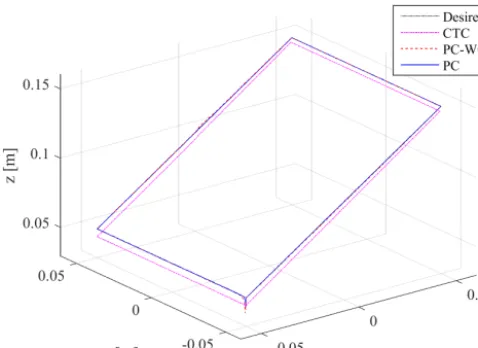
criteria have to be considered during trajectory planning for a robotic system, wherein polynomial functions are often used for interpolating the trajectory through several via points. Among various polynomial functions, the cubic polynomial is the lowest degree polynomial that can provide a trajectory with C2 smoothness, which guarantees continuous acceler-ation. Therefore, cubic polynomials are chosen for a poly-gon trajectory generation and tracking task. Further, the end-effector orientations are assumed to be zero for simplicity. The desired polygon trajectory is mathematically given as:
xr= (34)
−0.05
−0.05+4.8×10⁻³(t−25)2−1.28×10⁻⁵(t−25)3 0.05
0.05−4.8×10⁻³(t−75)2+1.28×10⁻⁵(t−75)3 −0.05
m m m m m
0≤t≤25 25< t≤50 50< t≤75 75< t≤100
100< t
yr= (35)
−0.05+4.8×10⁻³t2−1.28×10⁻⁵t3
0.05
0.05−4.8×10⁻³(t−50)2+1.28×10⁻⁵(t−50)3 −0.05
−0.05
m m m m m
0≤t≤25 25< t≤50 50< t≤75 75< t≤100 100< t
zr = (36)
0.05
0.05+4.8×10⁻³(t−25)2−1.28×10⁻⁵(t−25)3 0.15
0.15−4.8×10⁻³(t−75)2+1.28×10⁻⁵(t−75)3 0.05
m m m m m
0≤t≤25 25< t≤50 50< t≤75 75< t≤100 100< t
αr=0◦, βr =0◦, γr=0◦ ∀t (37)
In order to analyse the controller robustness, process and measurement noises are added in the form of Gaussian noises during the performance analysis. Similarly, an unknown ex-ternal disturbance vector has been considered and incorpo-rated in the simulations; it is a kind of random slowly varying
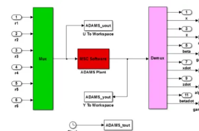
vector. For this analysis, it is assumed the estimated param-eters are only 90 % accurate with respect to the actual value. In addition, the manipulator initial velocities were set zero (start from rest) and the estimated system vectors were also considered as zero, while the initial desired and actual po-sitions and orientations were assumed to be the same. The virtual prototype (simulation) model of the proposed manip-ulator in the Simulink background is shown in Fig. 4 and is integrated (co-simulation) with the MSC Adams model of the same manipulator.
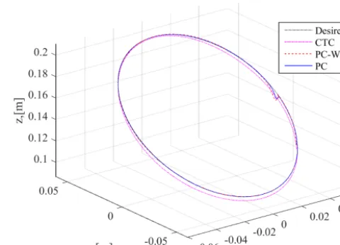
4.3 Simulation results and discussions
In this subsection, virtual prototype experiment results for the above-mentioned tasks are presented and discussed to in-vestigate the effectiveness and robustness of the proposed control scheme, which is expected to provide an intuitive, promising prospective of the proposed approach. To show the performance capability of the proposed robust control scheme, it is compared with other well-known scheme called a computed torque control (CTC) and is given by:
τc= ˆM(µ)
¨
µr+KPeµ+KD
˙
e
µ+ ˆC(µ,µ˙)µ˙+ ˆg(µ) (38)
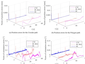
In order to understand the disturbance observer role, the con-troller performances further compared with and without the presence of the disturbance observer. The results of the con-troller performance analysis done in a virtual prototype are presented in Figs. 5, 6 and 7. The performances of different controllers are abbreviated as follows: the computed torque control is abbreviated as CTC, the proposed controller with and without disturbance observers are abbreviated as PC and PCWO. The task-space position trajectories of a circular path and a polygon path are presented in Figs. 5 and 6, respec-tively. The time trajectories of the norm of tracking errors are presented in Fig.7. So as to understand the performance of the controller in a more quantitative way, the root-mean-square error analysis is performed by varying the controller parameters and working conditions. The root-mean-square (RMS) values of the vector of tracking errors of the end-effector pose are used as a performance measure quantity for the controller comparison and mathematically, it is given as:
κrms=
v u u u t n P i=1
(xri−xi)2+(yri−yi)2+(zri−zi)2
n (39)
ϕrms=
v u u u t n P i=1
(αri−αi)2+(βri−βi)2+(γri−γi)2
n (40)
Figure 7.Time trajectories of the norm of tracking errors.
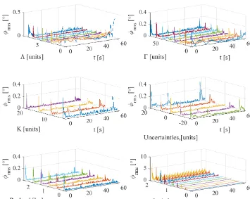
Figure 8.Controller parameter sensitivity and robustness analysis results: Parameter variations vs. Root-mean-square error of end-effector positions.
are high at the initial stage which is due to the presence of zero observer values and non-zero gravity compensation (presence of 1g(µ)=g(µ)− ˆg(µ)). However, over a pe-riod of time, the proposed controller compensates this ef-fect due to the centralized PID control vector and the distur-bance observer. But in the case of computed torque control, this effect could remain and because of the only PD
con-Figure 9.Controller parameter sensitivity and robustness analysis results: Parameter variations vs. Root-mean-square error of end-effector orientations.
Figure 10.Sensitivity and robustness analysis results: Time trajectories of the norm of the end-effector position errors.
observer by applying the proposed controller. The same trend is approximately followed in the polygon path as well. From the root mean square error analysis of orientation, it is found that the proposed controller reduced the end-effector orien-tation errors to 0.05◦as compared to other controllers. Since the desired end-effector orientations are zero in the case of polygon/cubic polynomial path, the differences in the orien-tation errors of all three controllers are very less.
Further to understand the robustness and behaviour of the proposed control scheme when there are variations in its con-troller parameters, payload, uncertainty and dynamic work-ing conditions, the robustness and sensitivity analyses are conducted by tracking a circular trajectory of the end-effector positions as mentioned earlier with different operating con-ditions. Apart from varying the controller parameters, the working conditions are also varied in this analysis.
The percentage of parameter uncertainties is varied from −20 to +20 %, i.e., the gravity vector, inertia and Corio-lis matrices are inaccurately known with these percentage variations. Similarly, for the payload variations, an addi-tional mass added to the end-effector and the value of the mass is varied from 0 to 2.5 kg. In addition, the frequency of the circular trajectory as mentioned in Eq. (32), ωvalue is also varied 0.1 to 2, instead of keeping a constant value as 0.1. The controller parameter sensitivity and robustness analysis results are presented in Figs. 8–11. The RMS val-ues of end-effector position and orientation errors are plot-ted in Figs. 8 and 9, respectively. Similarly, time histories of the end-effector position and orientation errors are plotted in Figs. 10 and 11 respectively. These plots show that the error variations are very minimal for the parameter variations, ex-pect at higher speeds of operations. From overall results, it is observed that the proposed controller is robust enough for the parameter uncertainties, un-modelled dynamics and payload variations.
5 Conclusions
In this paper, the inverse dynamic model and a robust adap-tive motion control scheme of a 6-DOF spatial 3-RPRS par-allel manipulator system in the presence of parametric un-certainties and external disturbances have been investigated. The proposed control strategy was designed to track the given desired end-effector trajectory in the task-space with
minimal errors. The effectiveness of the proposed controller was verified by simulation. From the obtained numerical simulation results, the strength of proposed control scheme can be summarized as follows:
– Proposed controller increases the overall stability of closed loop system as compared to conventional con-trollers.
– Poor knowledge of the system parameters will be suffi-cient to design the controller.
– Proposed control scheme provides great immunity to the external disturbances and parameter uncertainties as compared to conventional controllers.
– Proposed controller has simple control structure and de-sign. Hence, it can be used for time implementation with a low-cost microprocessor.
– The proposed controller can also be applied to other kinds of parallel manipulators.
Future work will concentrate on the real implementation of the proposed controller to our in-house fabricated manipu-lator prototype system. Also, in upcoming studies, the eval-uation shall be made between the proposed scheme and the latest published studies for this kind of manipulator to ex-amine whether this technique is robust when compared with new and recent controllers and the well-tuned proportional controller with the feedforward compensation.
Appendix A: Nomenclature
Variable/Symbol Description PO
P The position vector of the frameP with respect to the frameO O
PR The rotation matrix of the frameP with respect to the frameO
Px, PyandPz Positions of the end-effector with respect to the fixed base platform coordinate system
α, βandγ The roll, pitch and yaw angles of the end-effector with respect to the fixed base platform coordinate system
µ Vector of the task-space displacements (both translational and rotational displacements or in other words positions and orientations of the end effector )
q The vector of actuator coordinates (joint-space displacements) namely rotation angles and translation displacements of the manipulator
θi Rotation angle ofith active rotary joint
di Translational displacement ofith active translational or prismatic joint
Ci The position coordinates of the spherical joints on the mobile platform with respect to the fixed
coordinate system
ri The distance between end-effector point to theith spherical joint on the mobile platform
ψi The angle between end-effector frame to theith spherical joint on the mobile platform
δi The vertical offset distance between the translational joint axis to the rotary axis of theith leg
li The link length of theith leg
J(µ) The inverse Jacobian matrix of the manipulator KE The total sum of the kinetic energy of the mechanism PE The total sum of the potential energy of the mechanism
µiandµ˙i The corresponding task-space displacement and velocity of theith task-space variable, respectively.
M(µ) Inertia matrix
C(µ,µ˙) Centripetal and Coriolis force matrix g(µ) Gravitational force vector
τ Input vector
f(µ,µ˙) Frictional force vector;
τc Control (actuator) input vector in task-space;
τd Disturbance vector in task-space (which includes external disturbances and internal uncertainties namely parameter variations, noises, etc.)
ρ Vector of inputs (control inputs) in joint-space
Kand0 Controller and observer gain matrices of the proposed controller, respectively. ¨
µv Virtual desired acceleration vector. ¨
µr,µ˙r andµr The desired task-space acceleration, velocity and position vectors, respectively.
e
µandeµ˙ Vector of task-space position errors and velocity errors, respectively. 3 Centralized PID control gain matrix of the proposed control scheme. ξ Centralized proportional-integral-derivative (PID) control input vector. η Vector of lumped disturbances of the manipulator.
ˆ
Competing interests. The authors declare that they have no con-flict of interest.
Acknowledgements. The financial support of the first author as a Humboldt Research Fellow by the Alexander von Humboldt (AvH) Foundation, Germany is gratefully acknowledged.
Edited by: Andreas Müller
Reviewed by: three anonymous referees
References
Abdellatif, H. and Heimann, B.: Computational efficient inverse dynamics of 6-DOF fully parallel manipulators by using the Lagrangian formalism, Mech. Mach. Theory, 44, 192–207, https://doi.org/10.1016/j.mechmachtheory.2008.02.003, 2009. Alizade, R. I. and Tagiyev, N. R.: A forward and reverse
dis-placement analysis of a 6-DOF in-parallel manipulator, Mech. Mach. Theory, 29, 115–124, https://doi.org/10.1016/0094-114X(94)90024-8, 1994.
Bonev, I. A.: Analysis and design of 6-DOF 6-PRRS parallel manip-ulators, Master Thesis, Kwangju Institute of Science and Tech-nology, Kwangju, 1998.
Briot, S., Arakelian, V., and Guégan, S.: PAMINSA: A new family of partially decoupled parallel
ma-nipulators, Mech. Mach. Theory, 44, 425–444,
https://doi.org/10.1016/j.mechmachtheory.2008.03.003, 2009. Byun, Y. K. and Cho, H. S.: Analysis of a novel 6-DOF, 3-PPSP
parallel manipulator, Int. J. Robot. Res., 16, 859–872, 1997. Carbonari, L., Battistelli, M., Callegari, M., and Palpacelli, M.-C.:
Dynamic modelling of a 3-CPU parallel robot via screw theory, Mech. Sci., 4, 185–197, https://doi.org/10.5194/ms-4-185-2013, 2013.
Dasgupta, B. and Mruthyunjaya, T.: The Stewart platform manipulator: a review, Mech. Mach. Theory, 35, 15–40, https://doi.org/10.1016/S0094-114X(99)00006-3, 2000. Davliakos, I. and Papadopoulos, E.: Model-based
con-trol of a 6-dof electrohydraulic Stewart–Gough
platform, Mech. Mach. Theory, 43, 1385–1400,
https://doi.org/10.1016/j.mechmachtheory.2007.12.002, 2008. Honegger, M., Brega, R., and Schweizer, G.: Application of a
nonlinear adaptive controller to a 6 DOF parallel manipulator, in: Proceeding of the 2000 IEEE International Conference on Robotics and Automation, San Francisco, 2000.
Isaksson, M., Brogårdh, T., Watson, M., Nahavandi, S., and Crothers, P.: The Octahedral Hexarot – A novel 6-DOF parallel manipulator, Mech. Mach. Theory, 55, 91–102, https://doi.org/10.1016/j.mechmachtheory.2012.05.003, 2012. Kelly, R., Santibanez, V., and Loria, A.: Control of Robot
Manipu-lators in Joint Space, Springer, London, UK, 2005.
Kim, D. H., Kang, J. Y., and Lee, K.-II.: Robust track-ing control design for a 6 DOF parallel manipulator, J. Robotic Syst., 17, 527–547, https://doi.org/10.1002/1097-4563(200010)17:10<527::AID-ROB2>3.0.CO;2-A, 2000.
Kim, H. S., Cho, Y. M., and Lee, K.-II.: Robust nonlinear task space control for a 6 DOF parallel manipulator, Automatica, 41, 1591– 1600, https://doi.org/10.1016/j.automatica.2005.04.014, 2005. Liu, X. J., Wang, J., Gao, F., and Wang, L. P.: Mechanism design
of a simplified 6-DOF 6-RUS parallel manipulator, Robotica, 20, 81–91, https://doi.org/10.1017/S0263574701003654, 2002. Merlet, J.-P.: Parallel Robots, Kluwer Academic Publishers, Boston,
2000.
Nag, A., Mohan, S., and Bandyopadhyay, S.: Forward kinematic analysis of the 3-RPRS parallel manipulator, in: New Trends in Mechanism and Machine Science: Theory and Industrial Appli-cations, edited by: Wenger, P. and Flores, P., Springer Interna-tional Publishing, 103–111, https://doi.org/10.1007/978-3-319-44156-6, 2017.
Nguyen, A. V., Bouzgarrou, B. C., Charlet, K., and Béakou, A.: Static and dynamic characterization of the 6-Dofs parallel robot 3CRS, Mech. Mach. Theory, 93, 65–82, https://doi.org/10.1016/j.mechmachtheory.2015.07.002, 2015. Nguyen, C. C., Antrazi, S. S., Zhou, Z. L., and
Camp-bell, C. E.: Adaptive control of a Stewart platform-based manipulator, J. Robotic Syst., 10, 657–687, https://doi.org/10.1002/rob.4620100507, 1992.
Pierrot, F.: A new design of a 6-DOF parallel robot, Journal of Robotics and Mechatronics, 2, 308–315, https://doi.org/10.20965/jrm.1990.p0308, 1990.
Ryu, S. J., Kim, J., Hwang, J., Park, C., Kim, J., and Park, F. C.: ECLIPSE: An Overactuated Parallel Mechanism for Rapid Ma-chining, in: Proceedings of the 12th CISM-IFTOMM Sympo-sium on the Theory and Practice of Robots and Manipulators, Paris, 1998.
Slotine, J. J. E. and Li, W.: Applied Nonlinear Control, Prentice-Hall, London, 1991.
Tahmasebi, F. and Tsai, L-W.: Six-degree-of-freedom Parallel “Minimanipulator” With Three Inextensible Limbs, U.S. Patent No. 5,279,176, 1994.
Ting, Y., Chen, Y. S., and Jar, Y. S.: Modeling and control for a Gough–Stewart platform CNC machine, J. Robotic Syst., 21, 609–623, https://doi.org/10.1002/rob.20039, 2004.
Uchiyama, M.: A 6 d.o.f. parallel robot HEXA, Adv. Robotics, 8, 601–601, https://doi.org/10.1163/156855394X00293, 1993. Venkatesan, V., Singh, Y., and Mohan, S.: Inverse Kinematic
Solu-tion of a 6-DOF (3-RPRS) Parallel Spatial Manipulator, in: Pro-ceedings of the 3rd Joint International Conference on Multibody System Dynamics – IMSD 2014, Busan, 2014.
Wu, D. and Gu, H.: Adaptive Sliding Control of Six-DOF Flight Simulator Motion Platform, Chinese J. Aeronaut., 20, 425–433, https://doi.org/10.1016/S1000-9361(07)60064-8, 2005. Yang, C., Huang, Q., Jiang, H., Peter, O.O., and Han, J.:
PD control with gravity compensation for hydraulic 6-DOF parallel manipulator, Mech. Mach. Theory, 45, 666–677, https://doi.org/10.1016/j.mechmachtheory.2009.12.001, 2010. Zhang, D.: Parallel Robotic Machine Tools, Springer, London,