Abstract
The increasing number of demanding consumer video applications, as exemplified by cell phone and other low-cost digital cameras, has boosted interest in no-reference objective image and video quality assessment (QA) algorithms. In this paper, we focus on no-reference image and video blur assessment. We consider natural scenes statistics models combined with multi-resolution decomposition methods to extract reliable features for QA. The algorithm is composed of three steps. First, a probabilistic support vector machine (SVM) is applied as a rough image quality evaluator. Then the detail image is used to refine the blur measurements. Finally, the blur information is pooled to predict the blur quality of images. The algorithm is tested on the LIVE Image Quality Database and the Real Blur Image Database; the results show that the algorithm has high correlation with human judgments when assessing blur distortion of images.
Keywords:No-reference blur metric, Gradient histogram, Multi-resolution analysis, Information pooling
1. Introduction
With the rapid and massive dissemination of digital images and videos, people live in an era replete with digitized visual information. Since many of these images are of low quality, effective systems for automatic image quality differentiation are needed. Although there are a variety of effective full-reference (FR) quality assessment (QA) models, such as the PSNR, the structural similarity (SSIM) index [1,2], the visual information fidelity index [3], and the visual signal-to-noise ratio (VSNR) [4], models for no-reference (NR) QA have not yet achieved performance that is competitive with top performing FR QA models. As such, research in the area of blind or NR QA remains quite vital.
There are many artifacts that may occur in a distorted image, such as blocking, ringing, noise, and blur. Unlike FR QA, where a reference is available to test against any distortion, NR QA approaches generally seek to capture one or a few distortions. Here we are mainly concerned with NR blur assessment, which remains an important problem in many applications. Generally, humans tend to conclude that images with more detail are of higher quality. Of course, the question is not so simple, since
blur can be space-variant, may depend on depth-of-field (hence effect foreground and background objects differ-ently), and may depend on what is being blurred in the image.
A number of NR blur indices have been developed, the majority of which are based on the analyzing lumi-nance edges. For example, the sharpness measurement index proposed by Caviedes and Gurbuz [5] is based on local edge kurtosis. The blur measurement metric pro-posed by Marziliano et al. [6] is based on analyzing of the width or spread of edges in an image, while their other work is based on an analysis of edges and adjacent regions in an image [7]. Chuang et al. [8] evaluate blur by fitting the image gradient magnitude to a normal dis-tribution, while Karam et al. develop a series of blur metrics based on the different types of analysis applied to edges [9-13].
Other researchers have studied blur assessment by fre-quency domain analysis of local DCT coefficients [14], and of image wavelet coefficients [15-17]. These meth-ods generally rely on a single feature to accomplish blur assessment. While some of these algorithms deploy sim-ple perceptual models in their design [7,9,11,12,17], a theme that we extend in our approach. Specifically, we use a model of neural pooling of the responses of corre-lated neuronal populations in the primary visual cortex
* Correspondence: [email protected]
Department of Electrical & Computer Engineering, Laboratory for Image and Video Engineering, The University of Texas at Austin, Austin, TX, USA
[18]. The use of multiple features combined using machine learning methods has also been studied [19,20]. We are also inspired by recent progress on utilizing natural scene statistics (NSS) to improve image proces-sing algorithms. Natural images obey specific statistical laws that, in principle, might be used to distinguish nat-ural images from artificially distorted images [21]. In this regard, images that are blurred beyond a norm (e.g., more than the band limit provided by the normal human lens at optical center) may measurably depart from statistical “naturalness.” By this philosophy, we may anticipate that NR blur indices can be designed that analysis image statistics. Indeed, Sheikh et al. suc-cessfully used NSS for NR QA of JPEG-2000 distorted images [22]. In their work, specific NSS features drawn from the gradient histogram were used.
Here we develop a new blur assessment index that operates in a coarse-to-fine manner. First, a coarse blur measurement using gradient histogram features is deployed that relies on training a probabilistic support vector machine (SVM). A multi-resolution analysis is then used to improve the blur assessment, deploying a model of neural pooling in cortical area V1 [18]. The overall algorithm is shown to agree well with human subjectivity.
The rest of the paper is organized as follows: Section 2 describes the way in which NSS are used. Section 3 describes the coarse-scale NR blur index. Section 4 extends the metric using multi-resolution analysis. Sec-tion 5 explains the use of the neural pooling model. The overall NR blur index is evaluated in Section 6, and con-cluding remarks are given in Section 7.
2. Natural image statistics
Recent research on natural image statistics have shown that natural scenes belong to a small set in the space of all possible image signals [23]. One example of a natural scene property is the greater prevalence of strong image gradients along the cardinal (horizontal and vertical) orientations, in images projected from both indoor and outdoor scenes. A number of researchers have devel-oped statistical models that describe generic natural images [19] (including images of man-made scenes).
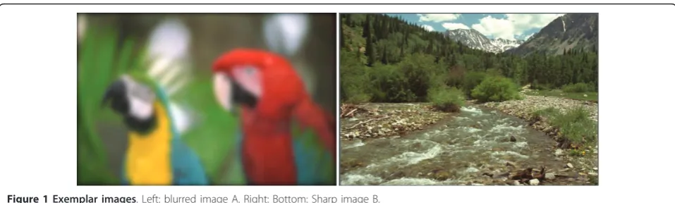
Although images of real-world scenes vary greatly in their absolute color distributions, image gradients gener-ally have heavy tailed distributions [24]. Natural image gradient magnitudes are mostly small, yet take large values significantly more often than a Gaussian distribu-tion. This corresponds to the intuition that images often contain large sections of smoothly varying intensities, interrupted by occasional abrupt changes at edges or occlusive boundaries. Blurred images do not have sharp edges, so the gradient magnitude distribution should have greater relative mass at small or zero values. By
example, Figure 1 shows a sharp and a blurred image. Figure 2 shows the distribution of their respective gradients.
Liu et al. [25] and Levin [26] have demonstrated that measurements on the heavy tailed distributions of gradi-ents can be used for blur detection. Liu et al. used the gradient histogram span as a feature in their classifica-tion model. Levin fits the observed gradient histogram using a mixture model.
3. Probabilistic SVM For blur assessment
Based on our discussion of NSS, we seek to evaluate the distance between the gradient statistics of an (ostensibly distorted) image and a statistical model of natural scenes. This distance can then be used for image QA.
A classification method is used to measure the dis-tance. We classify the images into two groups. One is tagged as“sharp” and the other as“blurred.” Using the probabilistic SVM classification model, confidence values are computed that represent the distance between the test image and the training set. A higher confidence value implies a higher certainty of the classification result. In this case, this means that the test sample is closer to the assigned class center, i.e., the statistic of the test image is closer to that of“sharp”or“blurred”images.
We chose to use a SVM [27] as our classification model. The main reason for using SVM is that it works well for classifying a few classes with few training samples. This is highly suitable for our application having only two classes. Moreover, SVM allows substitution of kernels to achieve better classification results. Although here we only use the default kernel, the possibility of modifying the kernel leaves room for performance improvement.
Due to the limited scope of the coarse evaluation of the image, we use the entire gradient histogram as a fea-ture, rather than simple measured parameter such as the mean or the slope of the histogram [25,26]. While this implies a fairly large number of features, it is not very large, and the small number of classes ensures reason-able computation. We describe the training procedure and the dataset used in Section 6.
After applying probabilistic SVM classification on an image, a label that indicates its class and a confidence score that indicates the degree of confidence in the deci-sion are obtained. Then the coarse quality score of the image is defined simply as:
QS−SVM(x) =
50 + 50·confidence, ifxis classified as sharp 50·(1 - confidence), ifxis classified as blurred (1)
4. Multi-resolution NR QA of blur
performance relative to single-resolution methods for image QA [2,4]. In the following, we modify QS-SVM using information derived from a multi-resolution decomposition.
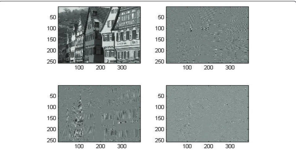
Applying a wavelet decomposition on an image is a natural way to examine local spatio-spectral properties that may reveal whether the image has been modified. For example, Figure 3 shows a sharp natural image decomposed by a two-level wavelet, while Figure 4 shows the decomposed blurred image. The sharp image is a high-quality image from the LIVE database. The blurred image was modified by a Gaussian low-pass filter. We used the 2D analysis filter bank devel-oped in [28] to analyze the image. From Figures 3 and 4, it is apparent that the sharp image contains signifi-cant horizontal and vertical energy in the high bands, while the blurred image does not. As a simple measure of sharpness, we sum the horizontal and vertical responses in the high band to produce a detail map. Figure 5 shows the detail map derived from the sharp image in Figure 3.
A quality (or sharpness) score that combines QS-SVM with multi-resolution analysis follows:
Blur quality score =(QS - SVM)r0 N
i=1
(DSi)ri (2)
where N is the number of layers in the wavelet decomposition, and QS-SVM is the score obtained by analyzing the original image using the probabilistic SVM model described in the preceding. Further, DSi is the
detail scoreobtained from the detail map of layeri. The detail score at wavelet leveliis defined:
DSi= Wi
m=1
Hi
n=1∇i
(m,n)
Wi·Hi
(3)
whereWi andHi are the pixel dimensions of the
sub-band image that DSiis defined on, and ∇i(m,n) is the
gradient magnitude value of the subband image at coor-dinate (m, n).
Blur quality score is the final blur evaluation result, which is the weighted (by exponents) product of the full-resolution score QS-SVM and the values of DS from each layer. The parametersri are normalized
expo-nents: N i=0ri= 1.
5. Decoding the neural responses
Perceptual models have played an important role in the development of image QA algorithms. These have included image masking models [29], cortical decompo-sitions [30], extra-cortical motion processing [31], and foveation [29,32-34], among others.
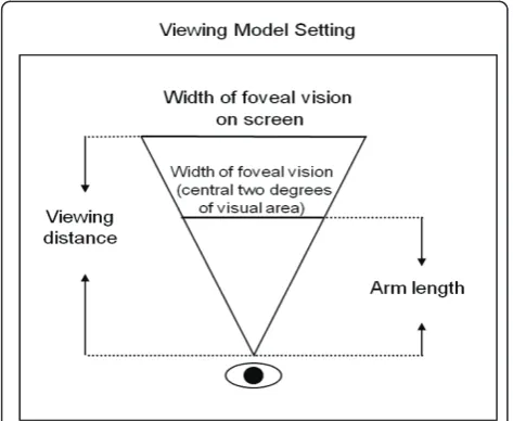
The visual model we will use is based on foveal (non-peripheral) processing of visual information. The central two degrees of high-resolution imagery that is projected onto the human fovea subtends roughly equivalent twice the width of a thumbnail at arm’s length [35]. In [9], a viewing model is used to derive the use of 64 × 64 blocks to approximate the size of image patches pro-jected from display onto the fovea (see Figure 6). In this Figure 1Exemplar images. Left: blurred image A. Right: Bottom: Sharp image B.
viewing model, a subject is assumed to be sitting in front of a 24” × 18” LCD screen with a resolution of 1680 × 1050 pixels. The width of foveal vision at arm’s length is assumed to be about 1.2”, while the viewing distance is assumed to fall in the range 36-54”
(approximately 2-3 times the screen height). The arm length of the viewer is assumed to be 33 in.. Then, the width of span of foveal vision on the screen falls between 76 (1050/18 × 1.31) and 116 (1050/18 × 2) pixels.
Figure 3Wavelet decomposition of natural image. Top left: low band response. Top right: horizontal high band response. Bottom left: vertical high band response. Bottom right: high band response.
Since a block size of 2nalong each dimension facilitates optimization and allows better memory management (aligned memory allocation), the choice of a 64 × 64 block size is a decent approximation. We then apply the blur QA method described in Section 4 on each of these blocks.
When a human observer studies an image, thus arriv-ing at a sense of its quality, she/he engages in a process of eye movement, where visual saccades place fixations at discrete points on the image. Image quality is largely
decided by information that is collected from these foveal regions, with perhaps, additional information drawn from extra-foveal information. The overall perception of qual-ity drawn from these fixated regions might be described as“attentional pooling,”by analogy with the aggregation of information from spatially distributed neurons. We utilize the results of a study conducted by Chen et al. [18] to formulate such an attentional pooling strategy. In this study, the authors examined the efficacy of different patch pooling strategies in a primate undergoing a visual (Gabor) target detection task.
The authors of [18] used voltage sensitive dyed images to measure the population responses in primary visual cortex of monkeys performing a demanding visual target detection task. Then, they evaluated the effects of different decoding strategies in predicting the target pattern from measured neural responses in primary visual cortex. The pooling pro-cess they considered used a linear summation model:
Xpooled=
n
i=1
wixi (4)
where wiis the weight applied to the neuronal
ampli-tude responsexi.
The pooling rules they studied are as follows:
1. Maximum average amplitude:wi≠0 only for the
patch having maximum average neuronal response amplitude.
Figure 5Detail map computed from image in Figure 3.
2. Maximum d’: wi ≠ 0 only for the patch having
maximumd’
3. Maximum amplitude:wi≠0 only for the site with
maximum amplitude in a given trial 4. Mean amplitude: wi= 1/n
5. Weighted average amplitude: wiis proportional to
the average amplitude response ofxi
6. Weightedd’:wiis proportional tod’
7. Optimal
where d’is the SNR of the neuronal responses across trials:
d=|ES−EN|
σS2+σN2
2 (5)
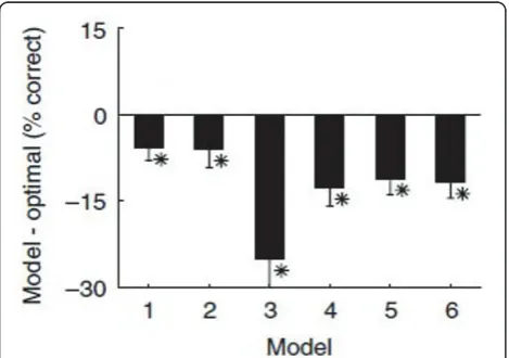
where ESis the mean response amplitude in target present trials (signal trials),ENis the mean amplitude of the response in target-absent trials (noise trials) andsS andsN are the corresponding standard deviations. The “optimal” pooling 7 is obtained under the assumption that the neuronal response at each site is Gaussian dis-tributed and independent across trials (although not across space and time within a trial). The optimal set of weights is defined as the product of the inverse of the response covariance matrix the vector of mean differ-ences in response between the signal and noise trials. Their experimental result is shown in Figure 7.
From Figure 7, we can see that the maximal average pooling rules (Rules 1 and 2) perform better than the trial maximum (Rule 3), average pooling rules (Rule 4) and weighted pooling rules (Rules 5 and 6). When applying analogous pooling rules to the image blur assessment problem, we observe that since distinct sig-nal and noise trials do not exist in our case (and in any
case the Gaussian assumption is questionable), so we cannot apply the optimal pooling rule (Rule 7). Further, the SNRd’is not available as required by Rules 2 and 6. Hence, we choose the maximum average amplitude as our pooling rule. The slight difference here is that with a single (algorithmic) “trial” an average amplitude value is not available, while the maximum amplitude (Rule 3) is unreliable. Instead, we use the average of the maxi-mump% of responses as a pooling strategy. The pooling strategy was applied only on activated neurons; hence we applied the pooling only on activated blocks, where a block was taken to be activated if the mean of the lumi-nance values in the block is higher than 20. Therefore, the final blur quality score is calculated as
Blur quality score =(QS−SVM)r0∗ N
i=1
Pool(DSi) ri (6)
where
Pool(DSi) =
n
k=1wkiDSki (7)
where DSkiis the detail response of block kfrom layer
i, and wki = 1/p if the detail responses of block kin
layer ibelong to the largest 10% of detail responses of all activated blocks in the layer; otherwisewki= 0. Here,
pis nominally set to 10. The blocking analysis and pool-ing are only applied on the multi-resolution part, since the NSS mentioned in Section 2 are based on the statis-tics of whole images.
6. Experiments and results
The LIVE image quality database [36] and the real blur image Database [37] were used to evaluate the perfor-mance of our algorithm. The experiments in Sections 6.1-6.3 were conducted on the LIVE database to gain insights into the performance of algorithms that com-bine different blur assessment factors. The performances are also compared to the performance of multi-scale SSIM (or MS-SSIM, a popular and effect FR QA method).
Then in Section 6.4, the Real blur database (586 Images) is used as a challenging test by which we com-pare our results with other NR QA blur metrics. The LIVE image database includes DMOS subjective scores for each image and several types of distortions. The experiment was performed only on the blur images (174 images). All of the images in the LIVE database are blurred globally. Samples of these images are shown in Figure 8. A total of 760 images were used for testing.
6.1. Performance of SVM Classification
To train the coarse SVM classifier, we used 240 training samples which were marked as“sharp”or“blurred.” The Figure 7 Comparison of detection sensitivity of candidate
training samples were randomly chosen and some of them are out-of-focus images. Due to the unbalanced quality of the natural training samples (there were more sharp images than naturally blurred images), we applied a gaussian blur to some of the sharp samples to gener-ate additional blurred samples. The final training set included 125 sharp samples and 115 blurred samples. The training and test sets do not share content.
When tagging samples, if an original image’s quality was mediocre, the image was duplicated; one copy marked as “blurred” and the other marked as“sharp,” with both images used for training. This procedure pre-vents misclassifications arising from marking mediocre image as “sharp” or “blurred.” This duplication was applied to lower the confidence when classifying med-iocre samples.
Note that DMOS scores of these images we are not required to train the SVM. Images were simply tagged as “blurred”or “sharp” to train the SVM. Likewise, the output of the probabilistic SVM model is a class type ("blurred” or “sharp”) and a confidence level. The class type and confidence level are used to predict the image quality score.
The algorithm was evaluated against the LIVE DMOS scores using the Spearman rank order correlation coeffi-cient (SROCC). The results are shown in Table 1.
In Table 1, QS-SVM means blind blur QA using probabilistic SVM, PSNR means peak signal to noise ratio, and MS-SSIM means multi-scale structure similar-ity index. To obtain an objective evaluation result, we compared our method to FR methods tested on the same database as in [4,38].
As can be seen, the coarse algorithm QS-SVM deliv-ered lower SROCC scores than the FR indices, although the results are promising. Of course, QS-SVM is not trained on DMOS scores, hence does not fully capture the perceptual elements of blur assessment.
6.2. Performance with multi-resolution decomposition We began by estimating which layers of the wavelet decomposition achieve the best QA result on the LIVE database. We found the correlations between the DS Figure 8Sample images from the LIVE image quality database. From top-left to bottom-right, increasing Gaussian blur is applied.
Table 1 Comparison of the performance of VQA algorithms
Prediction model SROCC
QS-SVM 0.6136
PSNR (FR) 0.7729
VSNR (FR) 0.932
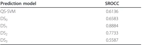
scores and human subjectivity for each layer. The per-formance numbers are shown in Table 2.
In Table 2, DS0 is the detail score computed from the original image. The experiment shows the SROCC score of DS1 to be significantly higher than for the other layers. The detail map at this middle scale appears to deliver a high correlation with human impression of image quality.
Next we combined the QA measurement in different layers, omitting level 3 because of its poor performance. Table 3 shows the results of several combinations of algorithms. The parametersriof each combination were
determined by regression on the training samples. Table 3 shows that, except for combination with QS-SVM, all other combinations with DS1 did not achieve higher performance than using only DS1. This result is consistent with our other work in FR QA, where we have found that mid-band QA scores tend to score higher than low-band or high-band scores. Adding more layers did not improve performance here. The highest performance occurs by combining DS1 with QS-SVM (r0 = 0.610,r1= 0.390), yielding an impressive SROCC score of 0.9105. Combination QS-SVM with DS2 (r0 = 0.683,r2= 0.317) also improved performance relative to DS2, suggesting that QS-SVM and the DS scores offer complementary measurements.
6.3. Performance with pooling strategy
We studied the performance of different pooling rules in our system. The system is described by (6), using maxi-mum p% pooling, average pooling (Rule 4 in Section 5), and weighted pooling (Rule 5 in Section 5), applied to QS-SVM·DS1. Using tenfold cross-validation with fixed parametersr0 = 0.610 andr1 = 0.390, the performance attained is given in Table 4. Table 4 shows that the
performance of using different pooling rules in our sys-tem is consistent with the results found in [18]. The maximum p% pooling method improves the perfor-mance (the SROCC score is increased from 0.9004 to 0.9248).
All parameters in our system were kept fixed (p= 10,
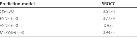
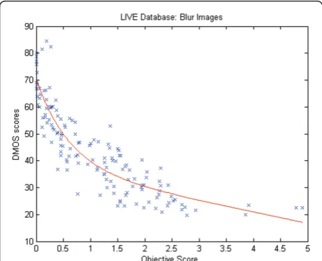
r0 = 0.610 and r1 = 0.390) to enable fair comparisons with other algorithms. The numberpcame from cross-validation across two databases. Table 5 illustrates the final performance of our algorithm as compared to other NR and FR blur metrics. The performance of our algorithm is better than PSNR and very close to CPBD [10] and to FR QA models when conducted on the blurred image portion of the LIVE Image Quality Data-base The plot of predicted objective quality (following logistic regression) against DMOS scores from the LIVE Image Quality Database is shown in Figure 9.
6.4. Challenging blur database
Our foregoing experiments on the LIVE database were by way of algorithm design and tuning, and not perfor-mance verification. To verify the perforperfor-mance of our algorithm, we conducted an experiment on a real blurred image database. The database contains 585 images with resolutions ranging from 1280 × 960 to 2272 × 1704 pixels.
The images in this database were taken by consumer cameras and are classified into five classes as “Unblurred”(204 images),“Out-of-focus”(142 images), “Simple Motion” (57 images), “Complex Motion” (63 images) and “Other” (119 images). The images in the
Table 2 QA performance using different layers
Prediction model SROCC
QS-SVM 0.6136
DS0 0.6583
DS1 0.8884
DS2 0.7733
DS3 0.5587
Table 3 QA performance using different combinations of layers
Prediction model SROCC
DS0·DS1 0.8884
DS1·DS2 0.8884
QS-SVM·DS1 0.9105
QS-SVM·DS1·DS2 0.9105
QS-SVM·DS2 0.8428
Table 4 QA performance numbers by tenfold cross-validation
Pooling rule SROCC
Maximump% 0.9248
Average 0.9004
Weighted 0.9080
Different pooling rules were applied on the blurred image portion of the LIVE Image Quality Database
Table 5 Summary of QA performance of different algorithms on the blurred image portion of the LIVE Image Quality Database
Prediction model SROCC
QS-SVM 0.6136
PSNR (FR) 0.7729
QS-SVM·DS1 0.9105
QS-SVM·Pool(DS1) 0.9352
VSNR (FR) 0.932
MS-SSIM (FR) 0.9425
“Out-of-focus” (142 images), “Simple Motion” (57 images), “Complex Motion” (63 images) and “Other” (119 images). The images in the“Out-of-focus” class are global out-of-focus images. The“Simple Motion”class has images that are blurred because of close-to-linear camera movements and the“Complex Motion”class has
each image.
We used tenfold cross-validation and report the SROCC numbers from applying several different pooling rules. As shown in Table 6, the maximump% pooling method yields the best performance (0.5858). Although the improvement is not significantly large, this method showed the best performance on both databases.
By examining the experimental results from the LIVE Image Quality Database and the Real Blur Image Data-base, we found that there is a significant performance difference of the models on these two databases. The LIVE database includes synthetically and globally blurred sample images. The task of performing QA on a globally blurred image is less complex and harder to relate to perceptual models. On LIVE, our proposed Figure 9Plot of predicted objective scores versus DMOS from
live image quality database.
method of pooling showed significant improvement (from 0.9 to 0.925). However, on the Real Blur Database, where the blurs are more complex, possibly nonlinear, and spatially variant, blur perception is more complex and probably more correlated with content (e.g., what is blurred in the image?). By example, in the partially blurred image shown in Figure 10 (bottom right), the rating is likely highly affected by image content, object positioning, probable viewer fixation, and so on.
When comparing the performance of our proposed algorithm with other blur assessment algorithms, we refer to the work conducted by Ciancio et al. [20]. In this work, they provided performance levels several algo-rithms, including a frequency-domain blur index [14], a wavelet-based blur index [15], a perceptually motivated blur index [7], a blur index using a human visual system (HVS) model [11], a local phase coherence blur metric [16], and their own Multi-Features Neural Network Classifier (MFNNC) blur metric [20]. The performance of CPBD [10] is also included. The performance results are shown in Table 7.
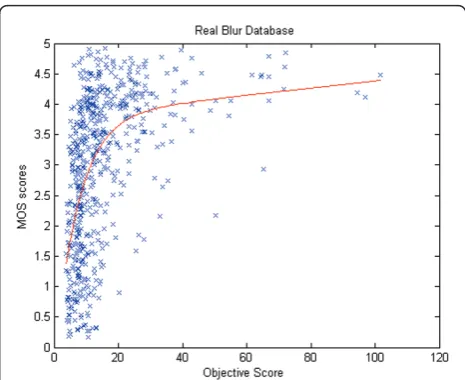
Table 7 shows that our proposed blur QA model deli-vers the best performance amongst the algorithms com-pared. Although the improvement does not achieve statistical significance as compared with other top-per-forming models, it consistently shows better perfor-mance across a large number of images and across databases. A scatter plot of the scores delivered by our model (following logistic regression) against the MOS scores from the Real Blur Database is shown in Figure 11 showing very good general agreement. Many of the images, such as Figure 12, contain difficult high level
content whose interpretation may depend on the obser-vers’preferences regarding composition (and that of the photographer).
7. Conclusion
The main contributions of this work are as follows. First, we found that the statistics of the image gradient histogram and a detail map from the image wavelet decomposition can be combined to yield good NR blur QA performance. Second, our results discuss that a per-ceptually motivated pooling strategy can be used to improve the NR blur index on assessing the blur images. Performance was demonstrated on the LIVE Image Quality Database and the Real Blur Image Database. As
Table 6 Blur QA performance of applying different pooling rules on real blur database
Pooling rule SROCC
Maximump% 0.5858
Average 0.5604
Weighted 0.5542
Table 7 Blur QA performance of different algorithms on real blur database
Algorithm SROCC
Frequency domain metric* 0.494
Wavelet-based metric* 0.524
Perceptual metric* 0.336
HVS based metric* 0.474
Local phase coherence metric* 0.523
MFNNC metric* 0.564
Proposed algorithm 0.586
CPBD 0.501
Algorithms marked by asterisk indicates their performance was reported in [20]
Figure 11Plot of predicted objective score versus MOS score of real blur image database.
Received: 15 September 2010 Accepted: 19 July 2011 Published: 19 July 2011
References
1. Wang Z, Bovik AC, Sheikh HR, Simoncelli EP:Image quality assessment: from error visibility to structural similarity.IEEE Trans Image Process2004, 13(4):600-612.
2. Wang Z, Simoncelli EP, Bovik AC:Multi-scale structural similarity for image quality assessment.IEEE Asilomar Conf. Signals, Systems, and Computers 2003, 1398-1402.
3. Sheikh HR, Bovik AC:Image information and visual quality.IEEE Trans
Image Process2006,15(2):430-444.
4. Chandler DM, Hemami SS:VSNR: a wavelet-based visual signal-to-noise ratio for natural images.IEEE Trans Image Process2007,16(9):2284-2298. 5. Caviedes JE, Gurbuz S:No-reference sharpness metric based on local
edge kurtosis.IEEE International Conference on Image Processing, Rochester, NY2002.
6. Marziliano P, Dufaux F, Winkler S, Ebrahimi T:A no-reference perceptual blur metric.International Conference on Image Processing, Rochester, NY 2002.
7. Marziliano P, Dufaux F, Winkler S, Ebrahimi T:Perceptual blur and ringing metrics: application to JPEG2000.Signal Process Image Commun2004, 19(2):163-172.
8. Chung Y, Wang J, Bailey R, Chen S, Chang S:A nonparametric blur measure based on edge analysis for image processing applications.IEEE Conf Cybern Intell Syst2004,1:356-360.
9. Narvekar ND, Karam LJ:A no-reference perceptual image sharpness metric based on a cumulative probability of blur detection.International
Workshop on Quality of Multimedia Experience2009.
10. Narvekar ND, Karam LJ:A no-reference image blur metric based on the cumulative probability of blur detection (CPBD).IEEE Trans Image Process 2011.
11. Ferzli R, Karam LJ:A human visual system based no-reference objective image sharpness metric.IEEE International Conference on Image Processing, Atlanta, GA2006.
12. Ferzli R, Karam LJ:A no-reference objective mage sharpness metric based on just-noticeable blur and probability summation.IEEE International
Conference on Image Processing, San Antonio, TX2007.
13. Varadarajan S, Karam LJ:An improved perception-based no-reference objective image sharpness metric using iterative edge refinement.IEEE International Conference on Image Processing, Chicago, IL1998.
14. Marichal X, Ma WY, Zhang H:Blur determination in the compressed domain using DCT information.IEEE International Conference on Image Processing, Kobe, Japan1999.
15. Tong H, Li M, Zhang H, Zhang C:Blur detection for digital images using wavelet transform.IEEE International Conference on Multimedia and EXPO 2004,1:17-20.
16. Ciancio A, Targino AN, da Silva EAB, Said A, Obrador P, Samadani R: Objective no-reference image quality metric based on local phase coherence.IET Electron Lett2009,45(23):1162-1163.
17. Wang Z, Simoncelli EP:Local phase coherence and the perception of blur.Advances in Neural Information Processing SystemsMIT Press, Cambridge; 2004, 786-792.
18. Chen Y, Geisler WS, Seidemann E:Optimal decoding of correlated neural population responses in the primate visual cortex. Nat.Neurosci2006, 9:1412-1420.
6:559-601.
25. Liu R, Li Z, Jia J:Image partial blur detection and classification.IEEE
International Conference on Computer Vision Pattern Recognition2008, 1-8.
26. Levin A:Blind motion deblurring using image statistics.Neural Information Processing Systems (NIPS)2006, 841-848.
27. LIBSVM:[http://www.csie.ntu.edu.tw/~cjlin/libsvm/].
28. Abdelnour AF, Selesnick IW:Nearly symmetric orthogonal wavelet bases. IEEE International Conference on Acoustic, Speech, Signal Processing (ICASSP) 2001.
29. Teo PC, Heeger DJ:Perceptual image distortion.IEEE International
Conference on Image Processing, Austin, TX1994.
30. Taylor CC, Pizlo Z, Allebach JP, Bouman CA:Image quality assessment with a Gabor pyramid model of the human visual system.SPIE
Conference on Human Vision and Electronic Imaging, San Jose, CA1997.
31. Seshadrinathan K, Bovik AC:Motion tuned spatio-temporal quality assessment of natural videos.IEEE Trans Image Process2010,19(2):335-350. 32. Lee S, Pattichis MS, Bovik AC:Foveated video quality assessment.IEEE
Trans Multimedia2002,4(1):129-132.
33. Wang Z, Bovik AC, Lu L, Kouloheris J:Foveated wavelet image quality index.SPIE’s 46th Annual Meeting, Proceedings of SPIE, Application of digital
image processing2001,XXIV:4472.
34. Cormack LK:Computational models of early human vision.InThe
Handbook of Image and Video Processing.Edited by: Bovik AC. Academic
Press; 2000:.
35. Mark F:Color Appearance ModelsAddison-Wesley, Boston; 1998, 7. 36. Sheikh HR, Wang Z, Cormack LK, Bovik AC:LIVE image quality assessment
database.Release 2[http://live.ece.utexas.edu/research/quality/subjective. htm].
37. BID–blurred image database.[http://www.lps.ufrj.br/profs/eduardo/ ImageDatabase.htm].
38. Wang Z, Wu G, Sheikh HR, Simoncelli EP, Yang EH, Bovik AC:Quality-aware images.IEEE Trans Image Process2006,15(5):1680-1689.
doi:10.1186/1687-5281-2011-3
Cite this article as:Chen and Bovik:No-reference image blur assessment using multiscale gradient.EURASIP Journal on Image and Video Processing20112011:3.
Submit your manuscript to a
journal and benefi t from:
7 Convenient online submission
7 Rigorous peer review
7 Immediate publication on acceptance
7 Open access: articles freely available online
7 High visibility within the fi eld
7 Retaining the copyright to your article