Gravitational Swarm Optimizer for Global Optimization
Anupam Yadava, Kusum Deepb, Joong Hoon Kimc,∗, Atulya K Nagard
aDepartment of Sciences and Humanites
National Institute of Technology Uttarakhand Srinagar-246174, Uttarakhand
India
bDepartment of Mathematics
Indian Institute of Technology Roorkee, Roorkee-247667 India
cSchool of Civil, Environmental and Architectural Engineering
Korea University, Seoul, South. Korea 136-713
dDepartment of Mathematics and Computer Science
Liverpool Hope University, Liverpool, U.K.
Abstract
In this article, a new meta-heuristic method is proposed by combining particle swarm optimization (PSO) and gravitational search in a coherent way. The advantage of swarm intelligence and the idea of a force of attraction between two particles are employed collectively to propose an improved meta-heuristic method for constrained optimization problems. Excellent constraint handling is always required for the success of any constrained optimizer. In view of this, an improved constraint-handling method is proposed which was de-signed in alignment with the constitutional mechanism of the proposed algorithm. The design of the algorithm is analyzed in many ways and the theoretical convergence of the algorithm is also established in the article.
The efficiency of the proposed technique was assessed by solving a set of 24 constrained problems and 15
unconstrained problems which have been proposed in IEEE-CEC sessions 2006 and 2015, respectively. The results are compared with 11 state-of-the-art algorithms for constrained problems and 6 state-of-the-art algo-rithms for unconstrained problems. A variety of ways are considered to examine the ability of the proposed algorithm in terms of its converging ability, success, and statistical behavior. The performance of the pro-posed constraint-handling method is judged by analyzing its ability to produce a feasible population. It was
concluded that the proposed algorithm performs efficiently with good results as a constrained optimizer.
Keywords: Particle Swarm Optimization, Gravitational Search Algorithm, Constrained Optimization,
Shrinking hypersphere, constrained handling
∗corresponding author
Email addresses:[email protected](Anupam Yadav),[email protected](Kusum Deep),
1. Introduction
Constrained optimization problems (COPs) are an important class of problems in the field of optimization, because many real-life problems arising in engineering, computer science, finance, and business science can be modeled as nonlinear constrained optimization problems. The formulation of any real-life problem into a constrained optimization problem involves the use of many parameters. Determination of the optimal value of each of these parameters is very important because together these values provide the solution to the problems. Mathematically, a constrained optimization problem can be formulated in the form of an objective function, which is constrained by some linear and nonlinear constraints. The following model provides the mathematical description of a nonlinear constrained optimization problem:
Min. or Max.f(x), x=[x1,x2,x3, ...,xD], (1)
subject to a set of inequality constraints
gk(x)60, k =1,2,3, ...q, (2)
as well as equality constraints
hk(x)=0, k= q+1,q+2, ...m, (3)
where objective function f is defined over subspace of a Ddimensional real vector space S ⊆ Rn and x is a
member ofD-dimensional vector space. A set ofqinequality constraints andm−qequality constraints, define
the feasible regionF ⊆S. Li 6 xi 6Uiare the lower and upper bounds of the decision variables in the domain
S, wherei=1 : 1 :D.
A class of optimization techniques is available in the literature for use with COPs. In principle, both de-terministic and nondede-terministic techniques are being used to solve COPs. Unfortunately, selected predefined assumptions of deterministic techniques restrict their applicability to a specific class of problems. This
re-striction directed us to focus on nondeterministic techniques, among which differential-free, nature-inspired
timization problems. Initially, these techniques were only used to solve unconstrained optimization problems.
Particle Swarm Optimization (PSO) [7, 28, 44], Differential Evolution (DE) [5, 33, 8], and the Gravitational
Search Algorithm (GSA) [45] are known to deliver excellent performance for unconstrained optimization
prob-lems, but have been found to perform variedly with COPs. In particular, the performance is strongly affected
when problems have to be solved at a high level of complexity. The complexity in COPs mainly occurs when the ratio of the search region to the feasible region is very small [29]. This level of complexity in problems
requires the combined use of different classes of algorithms to provide a more powerful constrained optimizer.
Many modifications and hybridizations intended to improve the efficiency and robustness of the algorithms
have appeared in the literature. Banks et al. [3] provide detailed information about the possible improvements of the PSO algorithm by hybridization, and they exhaustively discussed the major benefits of this development. Huang [23] improved the availability of the DE algorithm by evolving two subpopulation. Lwin and Qu [31] proposed a hybrid algorithm by integrating population-based incremental learning and DE for the solution of constrained portfolio selections.
The success of any constrained optimization algorithm mostly depends on the strength of the constraint-handling technique, the design of which has to be customized for an individual optimization algorithm. A few good constraint-handling mechanisms, that are capable of performing well, have been proposed. For example,
Deb [19] proposed an efficient constraint-handling approach for genetic algorithms, whereas Coello and Carlos
[14] published a comprehensive survey on constraint-handling approaches for a large number of optimization algorithms. Mezura-Montes and Coello [35] also furnished a detailed report in which they presented the future scope and trends of constraint-handling mechanisms. In [18] the design of a very good constraint-handling method for multiple swarm-based cultural PSO is described. The constraint-handling method discussed in [1] was successfully embedded within DE based on a penalty function. The FPBRM constraint-handling method proposed by Mun and Cho [40] for a modified harmony search algorithm also produced good results for optimization problems. The advantage of these algorithms lies in the fact that they were specifically designed for the technique being used for the optimization. This kind of constraint-handling mechanism is naturally compatible with the algorithms and enhances the performance of the optimizer. The overall message emerging
from these studies is that an effective constraint-handling method should be based on the individual algorithm
This research extends the concept of the recently proposed shrinking hypersphere PSO (SHPSO) [51] for unconstrained optimization and engineering design problems, as opposed to the method in [52], which was extended for constrained optimization problems. The performance of the SHPSO approach was improved using the GSA [45] and a global constrained optimizer was established with theoretical proof of its convergence and stability.
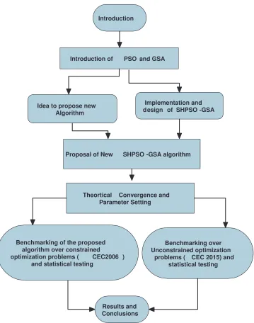
The organization of the paper is as follows. Section 2 briefly provides the concept of the GSA, and in sections 2.1 and section 2.2 the principles of PSO and SHPSO are discussed. Subsequently, in section 3, the proposed SHPSO-GSA is presented and section 4 contains a detailed theoretical and experimental analysis of the proposed algorithm. Section 5 discusses the proposed constraint-handling method and in section 6 the experimental results are discussed followed by the conclusions. A flow chart of the article is depicted in Fig. 2.
2. Gravitational Search Algorithm
The GSA [45] is a recent meta-heuristic algorithm for solving nonlinear optimization problems. It is inspired by Newton’s basic physical theory that states that a force of attraction works between every particle in the universe and this force is directly proportional to the product of their masses and inversely proportional to the square of the distance between their positions. In the GSA, each particle is equipped with four kinds
of properties: position, mass, active gravitational mass (Mai), and passive gravitational masses (Mpi) . The
position of the mass provides the solution of the problem. Gravitational mass and inertial mass can be evaluated using a fitness function. Each kind of mass follows the basic laws of physics:
i. Law of gravity: Each particle attracts every other particle and the gravitational force between two particles is directly proportional to the product of their respective mass and inversely proportional to the square of the distance between them [42].
ii. Law of motion: The current velocity of any mass is equal to the sum of the fractions of its previous
velocities and the variations in the velocity. Variation in the velocity of any mass is equal to the force exerted upon the system divided by the mass of inertia.
Inspired by the definitions above, we are able to define the physics of the GSA. Let the position of the ith
particle at any instant t in a D-dimensional search space be Xt
i(x t i1,x
t i2, ...,x
t
attraction (Fti jD) on theithparticle to jthparticle is defined as in the following equation
Fti jD =G t
× M
t pi× M
t a j
Rt i j
×(xtid −xtjd) (4)
where d = 1,2, ...D, Mt
pi is the passive gravitational mass related to i
th particle at time t, Mt
ai is the active
gravitational mass related to jth particle at time t, Gt is the gravitational constant at time t and Rt
i j is the
Euclidean distance between the two particlesiand j.
Rti j =kX t i,X
t jk
2
(5)
The value of gravitational constantGt can be calculated by Eq. 6
Gt =Gt0 ×exp((−α iter
itermax)) (6)
where α and G0 are descending coefficient and initial value, respectively. iter is the current iteration and
itermaxis the predefined maximum number of iterations.
The total force of attraction exerted by theithparticle at any instanttin a D-dimensional space is given by
Eq. 7
Fidt =
ps
X
i=1,i,j
rand()Fti jd (7)
whered= 1,2, ...D,rand() is the uniform random number generator in [0,1] and psis the number of agents.
which is introduced to provide the stochastic nature to the algorithm. By using the law of motion the
acceler-ation ofithparticle is given by the following equation:
actid = F
t id
Mt ii
(8)
whereMtiiis the inertial mass of theithparticle. The velocity and position of particles are calculated as follow:
Vidt+1= rand()×Vidt +actid (9)
xtid+1 = xtid +Vidt+1 (10)
calculated by the fitness evaluations. A greater mass can be treated as better particle and having higher force of attraction so that it can influence other particles with high level of attraction. The gravitational and inertial mass will be updated with the help of following equations:
Mai = Mpi = Mii for i=1,2...ps (11)
mti =
fitti−worst
t
bestt−worstt (12)
Mti = m
t i
Pps
i=1m t i
(13)
where fitti represents the fitness value of the i
th
particle at time t. bestt and worstt may be defined by the
following equations:
bestt = min(fittj), j∈ {1, ...ps} (14)
worstt =max(fittj), j∈ {1, ...ps} (15)
The exhaustive procedure of GSA is explained in Algorithm 1.
Algorithm 1Pseudo code of Gravitational Search algorithm Initialization
Randomly initialize (Xt
1,X t 2, ...,X
t
ps) of size psin search range [Xmin,Xmax]
Evaluate the fitness values (f itt1, f it2t, ..., f ittps) ofX(Agent)
Set iteration t=0
Reproduction and Updating
while Stopping Criterion is not satisfied do CalculateGt, bestt
, worstt andMt i
Calculate the total force in each directionFt i
Calculate theactiand velocity
Calculate the degree of infeasibility of each particle for i=1: psdo
Vit+1= rand()×Vit+acti Xt+1
i = X
t i +V
t+1 i
Evaluate the fitness values(f itt
i)ofX(Agent)
end for end while
GSA is very promising for unconstrained optimization problems; however, studies of the performance of the GSA over constrained optimization problems have indicated that, in terms of memory-less functionality, the performance of the algorithm is disappointing. This lack of intelligence provides the motivation to assemble the memory in the GSA by hybridizing it with PSO. In the next section, PSO is briefly explained.
2.1. Particle Swarm Optimization
Particle Swarm Optimization (PSO) is a nature-inspired stochastic population-based optimization search technique, inspired by the social behavior of fish and birds. PSO was first introduced by Kennedy and Eberhart in 1995 [26]. It uses the learning, information sharing, and position-updating strategy of each solution. It is very simple to implement on mathematical and computational platforms. The technique behaves analogously with bird flocking in that the search space is analogous to the flocking area of the bird; hence, each bird may be treated as a particle in the search space equipped with communicating abilities.
Let the position of the ith particle in a D-dimensional search space be Xit(xti1,xti2, ...,xtiD) with a flag of
velocityVit(vt
i1,v t i2, ...,v
t
id) at any moment t, where i = 1 to ps, where psis the swarm size. Let Pbest
t i and
Gbestt
i denote the latest best position of the particle(personal best) and global best at the momentt. Initially
Pbestt i andX
t
i are same. According to the theory of PSO, the position of the particle can be considered to have
changed when the linear combination of the aforementioned three influences has occurred. Mathematically, this can be expressed as:
Influence of(Vit)+Influence of(Gbestti−Xit)+Influence of(Pbest
t i−X
t
i) (16)
The formulated Eq. (16) is the velocity update equation, which can be written as:
Vit+1 =ωV t
i +c1r1(Xit−Gbest t
i)+c2r2(Xit−Pbest t
i) (17)
ωis the inertia weight,r1 andr2 are the uniform random number generators between 0 to 1. c1andc2are the
PSO parameters their values are mentioned in Table 1.
Xti+1 = Xit+Vit+1 (18)
Finally the velocity update equation in its formal expression is written in Eq. (17). The updated position of
explained in Algorithm 2.
Algorithm 2Pseudo code of Particle Swarm Optimization Algorithm
1: Initialization
2: Randomly initialize (Xt
1,X t 2, ...,X
t
ps) of size psin search range [Xmin,Xmax]
3: Initialize the velocity (V1t,V2t, ,Vpst ) in the range [Vmin,Vmax]
4: Set iteration t=0
5: Evaluate the fitness values (f itt
1, f it t
2, ..., f it t
ps) ofX
6: SetXit to bePbest=(Pbest1t,Pbestt2, ...,Pbesttps) for each particle
7: Set the particle with best fitness valueGbest
8: Reproduction and Updating
9: whileStopping Criterion is not satisfieddo
10: fori=1: psdo
11: Vt+1
i = ωV
t
i +c1r1(Pbest
t i−X
t
i)+c2r2(Gbest
t−Xt i)
12: Xit+1 = Xit+Vit+1 13: Pbestit+1= Pbestti
14: Gbestt+1 =Gbestt
15: Evaluate fitness(Xit+1)
16: if (fitness(Pbestt+1
i )<fitness(X
t+1
i )) then
17: Xt+1
i =Pbest
t+1 i
18: end if
19: if (fitness(Gbestt+1)<fitness(Pbestt+1
i )) then
20: (Pbestt+1
i )=Gbest
t+1
21: end if
22: end for
23: end while
Since it was initially proposed, the PSO technique has seen many modifications; for example, the first version [26] was later improved [47] by incorporating the concept of inertia weight into PSO. Subsequently, Eberhart and Shi [21] again proposed a method for tuning the parameters of the PSO algorithm. Clerc [9, 11, 10] introduced many major modifications to increase the usefulness of PSO. Many hybridized and modified versions of PSO were also proposed, such as Compact PSO [41], ICA-PSO [24], teaching and peer-learning PSO [30]. These hybridizations were implemented by incorporating the other heuristic techniques into PSO. A detailed study of the trajectory of PSO particles was discussed by Van den Bergh and Engelbrecht [50], and Zhang et al. [55] provided a theoretical analysis of PSO. Pluhacek et al. [43] designed a modified PSO driven by a multi-chaotic number generator. A new method referred to as SHPSO was proposed by Yadav and Deep [51, 52] based on the idea of the shrinking hypersphere versus particle generation. Additional noteworthy optimization algorithms, such as two-swarm COPSO [48], DSS-MDE [54], COMDE [39], DECV [36], time adaptive hybrid PSO [4], and A-DDE [37] were also presented in the literature.
Table 1: Parameter selection for the SHPSO
ω c1 c2 c3
0.9 1.49618 1.49618 1.01
GSA. This involved the proposal of a new equation for updating the velocity of PSO by incorporating the principles of GSA with the aim of improving the procedure for updating the positions of the particles. In the section 2.2, the important aspects of SHPSO [51, 52] are discussed.
2.2. Shrinking Hypersphere based PSO (SHPSO)
SHPSO was recently proposed by Yadav and Deep [51, 52]. This algorithm uses the shrinking hypersphere strategy in the search space to update the positions of the particles. SHPSO functions as follows
Let NGbest be the best (fittest) particle in the global hypershere [51] with the global best as the center.
Further, letNPbestbe the best (fittest) particle in the hypersphere withPbestas the center. CompareNGbest
& NPbest and select the fittest. Now apply both the velocity update and position update equations in such
a way that at each iteration, the radius of the hypersphere decreases from r to 0, which is proportional to
the total number of iterations as specified by the user. Thus, if a sufficiently large number of iterations are
performed, then the algorithm will converge to a point hypersphere. A description of the SHPSO is provided in Algorithm 3. The fine tuned parameter values [51] is listed in Table 1. In the next section the proposed SHPSO-GSA algorithms is discussed.
Recently, Hsing-Chih et al. [22] designed a hybrid algorithm by combining PSO with the GSA for un-constrained nonlinear optimization problems, which they tested against a benchmark of 14 problems. The
difference between the proposed approach and that of Hsing-Chih et al. [22] is that theirs involved
uncon-strained optimization, whereas this paper focuses on conuncon-strained optimization. Secondly, Hsing-Chih et al. [22] used standard PSO to hybridize GSA, in contrast to the SHPSO [51] used in this work. Finally, the benchmark functions used by Hsing-Chih et al. [22] only had two categories, i.e., uni-modal and multi-modal, whereas SHPSO [51] has already been tested over more complex functions proposed in IEEE CEC sessions. In this work, the IEEE CEC 2006 benchmark set of constrained optimization problems was employed to test the proposed SHPSO-GSA algorithm. In addition, the design of the mechanism of the proposed hybrid algorithm
is completely different from the version presented by Hsing-Chih et al. [22].
Algorithm 3Pseudo code of the shrinking hypersphere based PSO
1: Initialization
2: Randomly initialize (X1t,Xt2, ...,Xtps) of size psin search range [Xmin,Xmax]
3: Initialize the velocity (V1t,V2t, ...,Vtps) in the range [Vmin,Vmax]
4: Set iteration t=0
5: Evaluate the fitness values (f itt1, f it2t, ..., f ittps) ofX
6: SetXit to bePbest=(Pbestt
1,Pbest t
2, ...,Pbest t
ps) for each particle
7: Sort the Swarm based on the feasibility based rule [29]
8: i. The feasible solutions are listed in front of the infeasible solutions.
9: ii. The feasible solutions are sorted in ascending order of their objective function values.
10: iii. The infeasible solutions are sorted in ascending order of their degree of constrained violations.
11: Set the first particle in the second list toGbest
12: Generation of Hypersphere
13: Generate a hypersphere of radiusrcentered atGbest, generate psparticle inside the hypersphere
14: Evaluate the fitness value of each generated particle and choose the best feasible, name itNGbest
15: Again generate ps particles Hbest = (Hbestt1,Hbestt2, ...,Hbesttps) in the hypershpere of Pbestand
com-pute fitness ofHbest
16: Pbest= Best(Pbest,Hbest)
17: Reproduction and Updating
18: whileStopping Criterion is not satisfieddo
19: forido=1: ps
20: Vit+1= ωVit +c1r1(Pbestti−X
t
i)+c2r2(Gbest
t−
Xit)+c3r3(NGbestt−Xit)
21:
22: Xit+1 = Xit+Vit+1 23: Pbestit+1= Pbestti
24: Gbestt+1 =Gbestt
25: Evaluate fitness(Xit+1);
26: if fitness(Pbestti+1)<fitness(Xit+1)then
27: Xt+1
i =Pbest
t+1 i
28: end if
29: if fitness(Gbestt+1)<fitness(Pbestti+1)then
30: (Pbestt+1
i )=Gbest
t+1, Using feasibility based rule
31: end if
32: Again sort the swarm
33: Goto 12 UpdateHbestandNGbest. Using feasibility based rule
34: end for
seems to similar to the proposed article (SHPSO-GSA) but on careful observation both the articles have
sig-nificant difference both in idea as well as content. Table 2 presents a crisp comparison and differences between
these two algorithms Overall, the major difference between these algorithms are the idea of implementation
Table 2: Comparison between SHPSO-GSA and PSOGSA
Sr. No. SHPSO-GSA PSOGSA [38]
1. Hybridized with SHPSO and GSA Hybridized with SPSO and GSA
2. Proper justification and need of hybridization is
discussed
Not provided in the paper
3. The reason for each kind of influence is
dis-cussed before proposing the algorithm
No discussion and justification is provided, the authors have abruptly replaced the pbest with acceleration term of GSA
5. A detailed theoretical analysis is provided for
the convergence and stability of the algorithm
Not discussed
6. The idea is justified with many experiments Only few unconstrained problems are solved
7. Constrained problems of CEC 2006 and
uncon-strained problems of CEC 2015 is solved
Only simple unconstrained problems are solved with very less dimension
8. Compatible constraint handling mechanism is
proposed
Not applicable
and the current one is applicable for constrained as well as unconstrained problems while PSOGSA is applied only for unconstrained problems. The results of original SHPSO [51] in comparison to PSOGSA, the results are far better than PSOGSA. Therefore an outcome of the results of PSOGSA and SHPSO-GSA can be ana-lyzed easily and a conclusion can be drawn that SHPSO-GSA is better than PSOGSA based on experimental studies.
3. The Proposed Hybridized SHPSO-GSA Algorithm
3.1. Motivation of Hybridization
The fundamental motivation for designing the SHPSO-GSA algorithm was to utilize the memory-enabled behavior of PSO in the memory-less approach of GSA; i.e., GSA does not keep track of the path of any individual particle in its memory. The memory functionality was assembled into GSA by using it jointly with the recently proposed SHPSO. The advantage of the GSA is the constitutional diversity in the algorithm, which originates from the fundamental concept of defined acceleration of a particle. Because the acceleration of a particle is a function of the force experienced by the existing gravitational field due to the other particles and
its mass. On the other hand, when processing COPs, the performance of the GSA is strongly affected by the
feasible and search regions is very small, the GSA does not behave well, because the mass values of particles
behave similarly, thereby diluting the effect of the gravitational field over the particles. This results in the
particles ceasing their movement at places of less importance. In contrast, the ability of PSO to memorize the trajectory of a particle avoids the looping of the particles in some interval. This discussion is experimentally justified as follows. Plots of the GSA and the proposed SHPSO-GSA (in the next section) have been applied
to solve the problems g01 and g02 [29], and the fitness value and infeasibility of the last population (for a
population size of 60), achieved after 4000 iterations, are compared. The results of the final population are depicted in Fig 3. The red stars in the figure show the fitness value of each particle in the last iteration and for each red star there is a corresponding blue circle vertically above the red star, to show the degree of infeasibility of each particle. The degree of infeasibility is calculated with the following equation:
G(xi)= m
X
j=1 Gj(xi)
where G(xi) is the degree of infeasibility of the ith particle xi and j is the number of constraints. For
the functiong01 the global fitness is ’-15’ [29] and the particles of the GSA are unable to reach the global
minimum even when the infeasibility of the particles is very high. However, when the same problem is solved by the SHPSO-GSA the result is excellent, with every particle able to reach the global minima with zero degree
of infeasibility. Fig. 4 depicts the same analysis for the problemg02 and again the particles of the GSA are not
able to reach to the global minima, whereas the SHPSO-GSA again produces an excellent result with 100% feasibility and optimum fitness. The major idea was to use exploitation capacity of the SHPSO and exploration ability of GSA algorithm together. In further sections it has been discussed that the designed hybrid performs in a good capacity in comparison to individual performances.
Apart from the above discussions the possible hybrid of SHPSO and GSA will increase the exploration ability. This is due to the exponential behavior of the acceleration term (See Eq. 29 and the idea is to uti-lize the exploratory nature of GSA. In order to measure the increased exploration ability the potential search
volume [28] of the SHPSO and SHPSO-GSA. The Potential search ranges forithparticle of SHPSO is given
by:
rd1i =|Gbestd−Xid|+|Pbestid−Xdi|+|NGbest−Xid| (19)
proposed in Eq. 23. Which is presented in Eq. 20
rd2i =acti +|Gbestt−Xdi|+|Pbestit−Xdi|+|NGbestd−Xid| (20)
The potential search volumes for theith particle, corresponding to SHPSO and SHPSO-GSA is given by
R1andR2respectively.
R1 =
d
Y
i
r1i (21)
R2 =
d
Y
i
r2i (22)
To understand the changed exploration ability of the proposed algorithm due to incorporation of the ac-celeration, the potential search volume is plotted against iterations, the total explored potential search volume of SHPSO and SHPSO-GSA are presented in Fig.5 and 6. These figures are plotted for sphere function over
[−100,100]25. Multiple runs are performed for this experiment and median curve is presented in the article. It
can be observed from the figures that the proposed hybrid has a better exploration ability in comparison to the original SHPSO algorithm.
3.2. Idea of Hybridization
The idea for implementing hybridization is to jointly influence the particles of the swarm by GSA as well as by SHPSO. The implementation of hybridization requires the movement of the particles to be controlled by the acceleration calculated from the gravitational search, i.e., the personal best (Pbest) of each particle and NGbest. These three influences are employed collectively to obtain the new position of the particles. As
in SHPSO, the position of the particle is updated by the newly calculated velocity, which is a combination of the global best, personal best,NGbest, and its previous velocity. The global best influence of the SHPSO
is replaced with the calculated acceleration of the particle. The removal of global best would not affect the
converging ability of the algorithm, due to the wayNGbestis designed; hence, it will effectively fulfill the need
of global best. Therefore, the proposed velocity update equation would be the combination of acceleration,
personal best, and the value ofNGbest.
Mathematically it can be formulated as: let Xt
i(x t i1,x
t i2, ...,x
t
iD) is the position of thei
thparticle in the
these choices are:
i. To move towards its current direction. .
ii. To move towards the particles suggested acceleration by gravitational search.
iii. To move towards the personal best of the particles.
iv. To move towards the NGbest of the population.
A combined influence is used, instead of moving toward any one of the direction listed above. Mathematically which can be expressed as
ω×Vit+ac t
i+(Pbest
t i−X
t
i)+(NGbest−X
t i)
with the help of Eq. 23, a new velocity and position update equation can be defined as:
Vit+1 =ω×Vit+c01×r1×acti+c 0
2×r2×(Pbestti −X
t i)+c
0
3×r3×(NGbest−Xit) (23)
where ω is the inertia weight, c01, c02 and c03 are the parameters whereas, r1, r2 and r3 are uniform random
number in the interval [0,1]. Using Eq. 23, the position update equation may be written as:
Xti+1 = Xit+Vit+1 (24)
An exhaustive procedure of SHPSO-GSA is presented in Algorithm 4. A logical flow chart of the proposed algorithm is also depicted in Fig. 7.
4. A Detailed Analysis of the Proposed Algorithm
This section presents a rigorous analysis of the proposed SHPSO-GSA. The effect of the modified velocity
updated equation, theoretical convergence, and converging ability is discussed in detail.
4.1. Effect of Proposed Velocity Update Equation
The effect of the proposed velocity update equation was studied by comparing its behavior with that of
Algorithm 4Pseudo code of SHPSO-GSA
1: Initialization
2: Randomly initialize (Xt
1,X t 2, ...,X
t
ps) of size psin search range [Xmin,Xmax]
3: Set iteration t=0
4: Evaluate the fitness values (f itt
1, f it t
2, ..., f it t
ps) ofX
5: for i=1: ps
6: SetXit to bePbest=(Pbest1t,Pbestt2, ...,Pbesttps) for each particle
7: CalculateGt, bestt
, worstt and Mt
i for i=1,2,. . .,ps
8: Calculate the total force in each directionFt
i
9: Calculate theacclti and velocity.
10: Calculate degree of infeasibility forG(Xt
i) each particleX
t i
11: Generation of Hypersphere
12: Generate a hypersphere of radiusrcentered atGbest
13: generate psparticle inside the hypersphere
14: Evaluate the fitness value of each generated particle
15: ChooseNGbestas a best feasible particle
16: Generate psparticlesHbest=(Hbestt
1,Hbest t
2, ...,Hbest t
ps) in the hypershpere ofPbest
17: Evaluate fitness ofHbest
18: Pbest= Best(Pbest,Hbest)
19: Replace each infeasible Xt
i to each feasible in the hypersphere ofPbestor replace with less infeasibility
20: Reproduction and Updating
21: while Stopping Criterion is not satisfied
22: Vt+1
i = ωV
t i +c
0 1r1ac
t i+c
0
2r2(Pbest
t i−X
t i)+c
0
3r3(NGbest
t −Xt i)
23: Xt+1
i = X
t i +V
t+1 i
24: Evaluate the fitness values (f itti) of X
25: UpdateGt
i, best
t
i, worst
t i M
t i
26: Calculate the total force in each directionFt
i
27: Calculate theacti and velocity
28: Again sort the swarm
29: Go to Step(2) UpdateHbestandNGbest, Using feasibility based rule
30: end while
the incorporation of acceleration in SHPSO-GSA is obvious when these two figures are compared. In Fig. 8 the velocity is seen to undergo damping at the end of the generations, which means the algorithm has good exploration abilities, although convergence is not achieved; however, in Fig. 9 the influence of acceleration on the velocity leads to enhanced exploration abilities as well as a good convergence for SHPSO-GSA. This comparative analysis of velocities is able to explain the benefit of incorporation of acceleration in the velocity update equation.
4.2. Convergence Condition for SHPSO-GSA
In this section, a theoretical analysis is performed for ensuring the convergence of the SHPSO-GSA
algo-rithm. Let X(t) be the position of any typical particle of the swarm at tth iteration. The velocity update and
position update equation are defined as:
Vit+1= ωVit+c01r1acti +c 0
2r2(Pbestti−X
t i)+c
0
3r3(NGbestt −Xit) (25)
Xti+1 = X t i +V
t+1
i (26)
Solving these two equations for a general particle
Xt+1−X(t)= ω(Xt −Xt−1)+c01r1×act+c02r2(Pbestt−Xt)+c03r3(NGbestt−Xt) (27)
⇒ Xt+1−(1+ω−c02r2−c 0
3r3)Xt −ωX
t−1= c0
1r1×act+c 0
2r2Pbestt+c 0
3r3Gbestt (28)
Eq. 8 defines the acceleration of a particle which is a function for Gravitational Constant (Gt), Mass (M) and
unit direction of (Xit −Xtj), the way all the entities are defined the acceleration (act) becomes a scalar multiple
ofe−t,
i.e. act ≈Ce−t (29)
whereCis a constant. Replacing the value ofact from Eq. 29 to Eq. 28, we have
Xt+1−(1+ω−c02r2−c 0
3r3)Xt −ωX
t−1 =c0 1r1Ce
−t+
c02r2Pbestt+c 0
The characteristic equation of Eq. 30 is given by
λ2−(1+ω−c0
2r2−c03r3)λ+ω= 0 (31)
λ1 = ν+
√
ν2−4ω (32)
λ2 = ν−
√
ν2−4ω (33)
whereν=(1+ω−c0
2r2−c 0
3r3), without loss of generality we may assume that att= 0,X(t)= X0and att= 1,
X(t)= X1. Using these initial conditions, the complementary solution of Eq. 30 will be
X∗t = Aλ t 1+Bλ
t
2 (34)
whereA= X0λ2−X1
λ1−λ2 andB= λ1X0−X1
λ1−λ2 . The particular solution will be
Xtp =
c01r1Ce−t
1+ω+ν +
c02r2Pbestt −c03r3NGbestt c02r2+c03r3
(35)
The general solution of the Eq. 30 will be
Xt = X∗t +X t
p (36)
Since
lim
t→∞
c01r1Ce−t
1+ω+ν →0
, thereforeXt will converge to a limit point if and only if
lim
t→∞Aλ t 1+Bλ
t
2 = 0 (37)
When ν2 − 4ω ≥ 0 then, λ1 and λ2 must be real. In this case a necessary and sufficient condition for the
convergence will bemaxkλ1 k,kλ2 k <1. In other case when they are not real thenλ1 = Reiθ andλ2 =Re−iθ,
whereR = √ω andθ = arctan
√ 4ω−ν2
ν , ω is a constant and in this case the necessary and sufficient condition
Hence in both the cases the presented algorithm converges with the above condition. Herer1,r2andr3are the
uniform random variables, therefore the expected values of thec01r1,c20r2andc03r3may be calculated with the
help of the probability density function of uniform random variable. therefore
E[c01r1]=c01
Z 1
0 x
1−0dx=
c01
2 (38)
similarly,
E[c02r2] = c02
2 (39)
E[c03r3] = c03
2 (40)
Hence using the expected values the limit becomes
lim
t→∞X t = c
0
2Pbest+c 0 3 c2+c3
(41)
In general for arbitrary values ofc0
2 andc 0
3any typical particle will converge to the following point
c0
2Pbest+c 0
3NGbest
c2+c3
This formally proves the trajectory of a particle of SHPSO-GSA will converge to a point which is a convex
combination ofPbestandNGbest.
4.3. Converging Ability
The converging ability of the proposed SHPSO-GSA algorithm was tested by applying it over the spherical function for a thirty-dimensional environment and the positions of the particles were observed after 200, 500, 800 and 1200 iterations are observed. A three dimensional environment of the above experiment is depicted in Fig. 10. Fig. 10(a) shows the initial population, In the Fig. 10(b) the position of the points are depicted
after 200 iterations and the position of the points reaches up to the order of 10−11. After 500 iterations the
position of the points converges to the order of 10−41, see Fig. 10(c). At the level of 800 iterations the position
converges to the order of 10−50as shown by the positions indicated in Fig. 10(d). Finally, after 1200 iterations
5. A New Constraint Handling Method
A parameter-free constraint-handling approach is used to ensure the feasibility of the particles. The degree
of constrained violation is evaluated by using Eq. 42 and the total degree of violation of an individual x is
evaluated by taking the sum of violations at each constraint, i.e. G(x) = Pm
j=1Gj(x). In each iteration the
swarm is sorted in the following three ways:
i. The feasible solutions are listed in front of the infeasible solutions.
ii. The feasible solutions are sorted in ascending order of their objective function values. The first particle of
the list will be theGbestand the best feasible particle in the global hypersphere will be theNGbest.
iii. The infeasible solutions are sorted in ascending order of their degree of constrained violations.
A schematic diagram is presented in Fig. 11 to facilitate understanding of the sorting method applied to the swarm. After sorting the swarm in the above manner, a new feasibility-based rule is added to process the swarm in the next iteration.
1. If all the particles in the swarm are feasible then process them to the next iteration after sorting in ascending order of their objective function value.
2. If there is an infeasible particle in the swarm, then the particles in the hypersphere of that individual will
considered for the replacement. For example, if at any iterationttheithparticle of the swarm is infeasible
then the particles of hypersphere ofPbestti will be sorted in ascending order of their feasibility, if any
feasible particle(s) is available in the hypersphere of Pbestti, it will replace the ith particle having the
least objective function value. In case there is no feasible particle inside the hypersphere ofPbestti, the
particle having the least constraint violation will be replaced with theithparticle.
The process will be repeated for all the particles in the main swarm for each constraint. Depending upon the feasibility-based rule discussed above, the total degree of constraint violation for each particle will be evaluated by using Eq. 42,
G(xi)= m
X
j=1
Gj(xi) (42)
where m is the number of constraints involved in the problem. In the next section, the results of the
Table 3: Fine tuned parameter values for SHPSO-GSA
ω c0
1 c
0
2 c
0
3 popsize
0.9 1.487 1.487 1.08 60
Table 4: State-of-the-art algorithms for comparison
Sr. No. Algorithm Sr. No. Algorithm
1 Basic PSO [47] 7 DSS-MDEa [54]
2 Trelea Type I [49] 8 COMDEb[39]
3 Trelea Type II; [49] 9 DECVc[36]
4 Clerc PSO [13] 10 A-DDEd[37]
5 Standard PSO (SPSO 2011) [12] 11 GSA [45]
6 SHPSO [51]
aMultimember DE with DSS
bConstrained optimization based on modified differential evolution algorithm cDifferential Evolution Combined Variants
dAdaptive Diversity Differential Evolution
5.1. Parameter Setting
The parameter values involved in the SHPSO-GSA has been determined from a rigorous fine tuning. The
fine tuning of the parameters are inspired from the original SHPSO algorithm, but still since in the
SHPSO-GSA a different component of acceleration is added to the algorithm, therefore based on the current scenario
a rigorous fine tuning has been performed for each choice of set of parameter values. After fine tuning it has
been concluded that the ranges1.47≤ c1 ≤ 1.49,1.47≤ c2 ≤1.49and1.00 ≤c3 ≤ 1.11for c1, c2 and c3 are
suitable for most of the test problems. ω = 0.9came out as a best choice. On the above ranges of parameter
values many experiments are done and the optimal value of the parameters are listed in Table 3.
In order to understand the SHPSO-GSA execution, a simulation process of an example is presented in Fig. 13. This provides a clear understanding of the proposed algorithm.
6. Experimental Analysis and Results
Table 5: System Configuration
PC Configuration Software Platform
Windows 7 Professional Matlab 7.10.0.499
Intel(R), Xenon(R) CPU (R2010a)
X5660, 2.80 GHz License No. 301017
6.1. Experimental Setup
All the algorithms were coded on the MATLAB platform. The results were obtained after 100 runs of the experiment were performed and analyzed. The results were evaluated for a maximum of 4000 iterations with an error tolerance of 0.00001 and the MATLAB-based seed function was used to generate the same initial population for each algorithm to justify the comparison. The experiments were conducted by using the system configuration listed in Table 5.
6.2. Benchmark Criteria
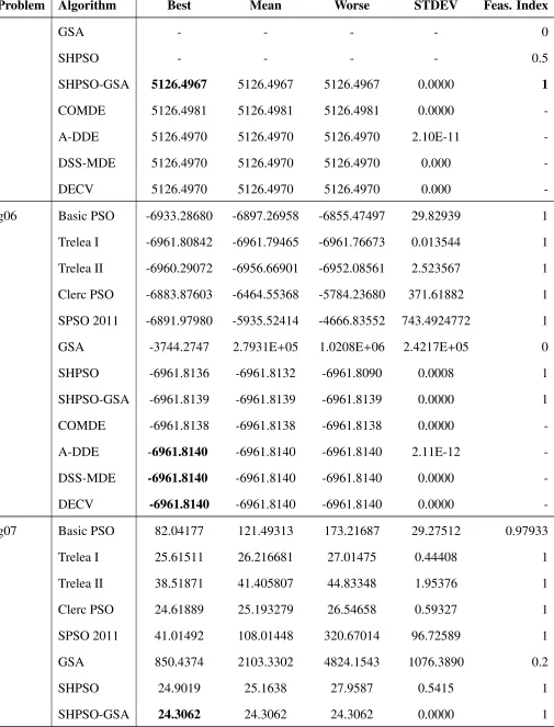
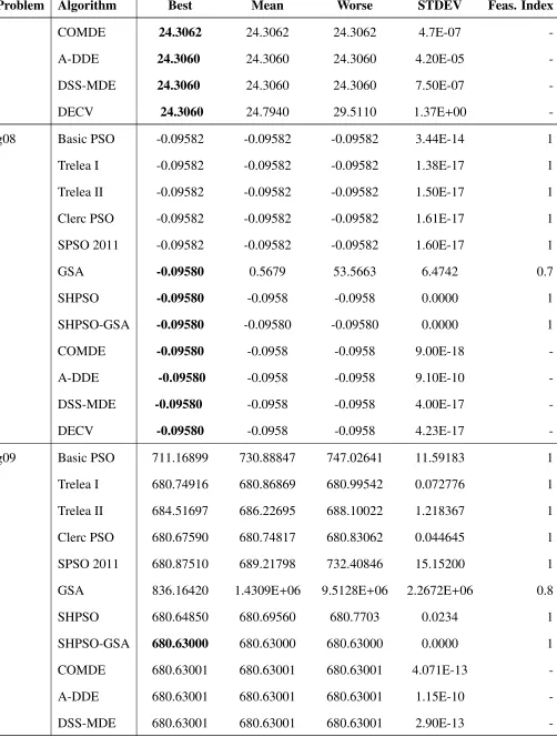
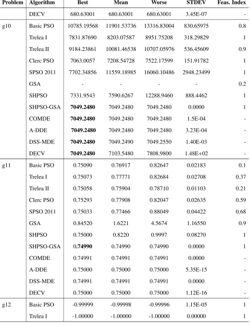
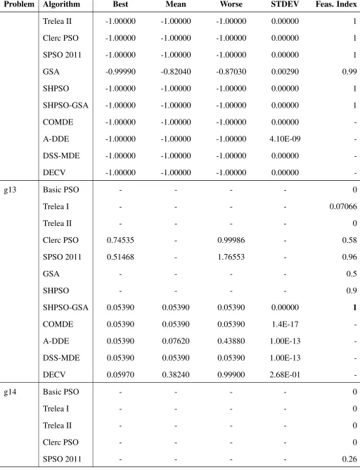
The results of SHPSO-GSA were compared with the other algorithms by recording the best, worst, mean, standard deviation, and feasibility index for each function, where the feasibility index is the ratio of the number of feasible particles in the last population to the total number of particles. Detailed results for each independent experiment are listed in Table 7. The feasibility rate, success rate, and success performance are calculated using the following formulae.
i. Feasible Run: A run during which atleast one feasible solution is recorded.
Feasibility Rate= No. of Feasible Runs
Total Runs
ii. Successful Run(Sruns): A run during which atleast one feasible solution is recorded meeting with|fit(x)−
fit(x∗)| ≤.0001 , where
f(x) is the known global minima and f(x∗) is the obtained minima.
Success Rate= No. of Successful Runs
Total Runs
iii. Success Performance (SP)= Avg. function evaluation of Sruns×Total runs
#Successful runs
To compare the results with other algorithms due care is taken as suggested by M. ˇCrepinšek et. al. [16, 15,
20, 17].
6.3. Results and Discussion
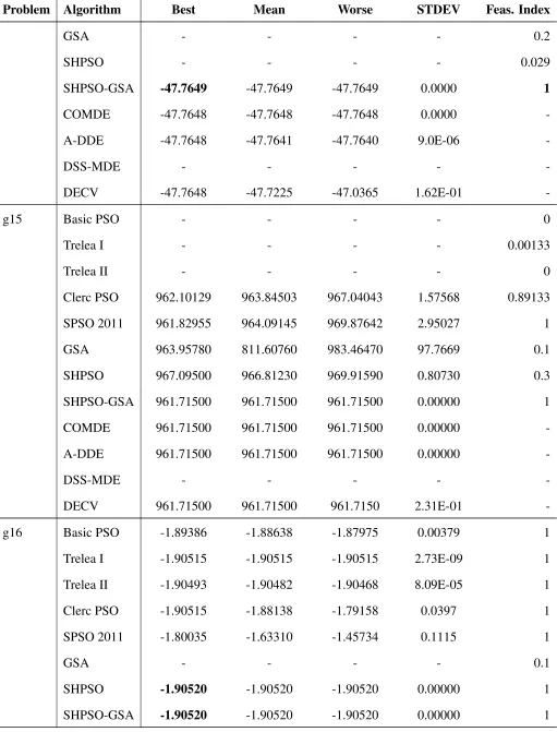
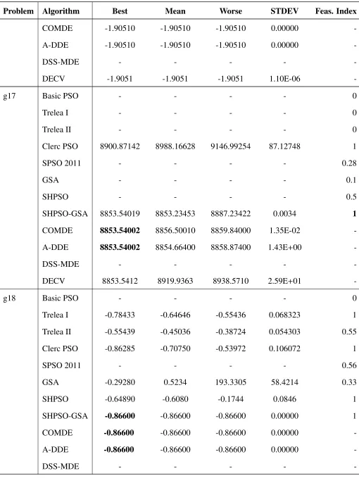
was fixed at 4000 with an error tolerance of 0.00001. Table 8 presents the attempt that was made to solve the 24 test problems taken from IEEE CEC 2006 [29] using the following approaches: basic PSO, Trelea I, Trelea II, Clerc PSO, SPSO 2011, GSA, SHPSO, and SHPSO-GSA. Out of the 24 problems, none of the
three algorithms were able to successfully solve two of the problems, namelyg20 andg22. Interestingly, the
infeasibility rate in these two cases was the lowest when SHPSO-GSA was used. For seven of the problems,
namelyg05, g13, g14, g15, g17, g21 and g23, neither the GSA nor SHPSO were able to provide a feasible
solution; however, the SHPSO-GSA could provide an optimal solution with an infeasibility rate of 0. For
seven of the problems, namelyg01,g06, g07,g10,g11,g16 andg18, the GSA was unable to reach a feasible
solution, whereas SHPSO and SHPSO-GSA provided an optimal solution with 0 mean infeasibility. For
the problemsg01, g04 to g16, g18, g19, g21, and g24 the SHPSO-GSA determined the best fitness value in
comparison with other algorithms. For the problemsg14 andg21 the SHPSO-GSA was the only algorithm
capable of providing a feasible solution for the problem. Thus, for 19 out of the 24 problems, the SHPSO-GSA
produced a 100% feasible population in its last iteration, thereby confirming the effectiveness of the designed
constraint-handling approach. The standard deviation of the results provided by SHPSO-GSA is ’0’ for 17 of the problems, which justifies the converging ability of the algorithm. There are four problems in which the SHPSO-GSA outperforms the COMDE, and it has an edge in 11 problems in comparison to A-DDE and is significantly more successful than DSS-MDE and DECV. The average number of successful runs in the function evaluation also exceeded those of COMDE, A-DDE, DSS-MDE, and DECV. Hence, we were able to conclude that the behavior of SHPSO-GSA is superior to the other PSO variants and the GSA based on the benchmark of selected problems.
6.4. Success
6.5. Convergence Plots
The convergence ability of SHPSO-GSA was compared with those of the other algorithms by plotting the
convergence graphs for the selected problemsg01,g02,g04,g06,g07,g08,g09 andg10, as shown in Figs. 14
and 15. The convergence of the proposed SHPSO-GSA is shown to be more rapid and more accurate in comparison to that of the SHPSO algorithm and the GSA.
6.6. Wilcoxon Signed Rank Test
In order to test the statistical validity of the results, pairwise Wilcoxon signed rank test [20] is used for
SHPSO-GSA Vs other algorithms. The test has been conducted withα = 0.05 significance level. The result
of the test is presented in Table 11. In the comparative table+, 0 and− shows the SHPSO-GSA has
outper-formed, equally performed and poorly in comparison to other algorithms respectively. The result justify that for majority of the problems SHPSO-GSA has better ranking than others.
6.7. ECD Plot
The algorithms were ranked on the basis of their successful performance by plotting the empirical
cumu-lative distribution ofS P/S Pbest listed in Table 10, whereS Pis the successful performance of theithproblem
andS Pbest is the best successful performance of the ith individual algorithm on the problem. The empirical
cumulative distribution (ECD) plots compare the ability of the algorithms to perform successfully, with the al-gorithm that reaches the top of the plot quickly will be considered as a best performer. Fig. 16 shows the ECD plots of all the algorithms, from which the available data representing successful performance, i.e., the prob-lems none of the algorithms succeeded in solving, are excluded. From Fig. 16 it is clear that the SHPSO-GSA performs excellently in comparison to the other algorithms because it reached the top of the graph quickly in comparison to the others.
7. Performance of SHPSO-GSA on Unconstrained Problems
In order to study the performance of SHPSO-GSA over unconstrained optimization problems. It is applied to solve CEC 2015 benchmark [6] expensive optimization test problems. All the 15 problems are solved and the results are compared with the state-of-the-art algorithms listed in Table 6
The results are listed in a form of best, worst, mean and standard deviation (stdev) of the fitness values of the corresponding problem in Table 12 and 13. The best result for each algorithm is presented in bold
Table 6: State of the art algorithms for comparing the results of the unconstrained optimization problems CEC 2015 [6]
Sr. No. Algorithm Sr. No. Algorithm
1. MVMO WOa[25] 4. MVMO WLb[25]
2. AncDEc [46] 5. iSRPSOd [32]
3. CMAES-Re [34] 6. CMAES-Df [34]
aMean-variance mapping optimization with out Local Search bMean-variance mapping optimization with Local Search cAn Ancestor based Extension to Differential Evolution dImproved SRPSO Algorithm
eCovariance Matrix Adaptation Evolution Strategy with specialized parameters fCovariance Matrix Adaptation Evolution Strategy with default parameters
F2,F3, F4,F5,F8,F9,F10,F11,F12,F13andF15all the recorded values of SHPSOGSA is better from other six
algorithms. For the functionsF7 andF14, except standard deviation all other entries of SHPSOGSA is better
than others. In case of 30D category, for the functions F1,F4, F10, F12, F13, F14 and F15 all the recorded
values of SHPSOGSA is better than other six algorithms. For function F2, F3,F5,F7, F11 the SHPSOGSA
records best fitness value than others. There is only one functionF6 for which the results of the SHPSOGSA
are competitive with other algorithms. Except this functions the output in all the streams starting form best fitness to standard deviation the performance of SHPSOGSA is excellent in comparison to other algorithms.
8. Algorithm Complexity
Algorithm 5Strategy for the calculation of algorithm complexity
1: Run the test program below:
2: fori=1:1000000do
3: x=0.55+(double)i;
4: x= x+ x;x= x/2;x= x∗x;x= sqrt(x);x=log(x);x=exp(x);x= x/(x+2); 5: end for
6: Computing time for the above=T0;
7: The average complete computing time for the algorithm=T1
8: The complexity of the algorithm is measured by: TT10
9: The complete computing time for the algorithm with 200000 evaluations of the same
10: D dimensional Function isT2
11: Execute step c five times and get fiveT2values. T2= Mean(T2)
12: The complexity of the algorithm is reflected by: T2,T1,T0, and (
T2−T1)
T0
The results of the algorithm complexity is listed in Table 14. The comparative analysis of the time com-plexity of SHPSO-GSA with MVMO WO and MVMO WL is presented in Table 15. The results are compared for 10D and 30D, it has been observed that the time complexity of SHPSOGSA is significantly less than other two algorithms. For most of the problems the time complexity of SHPSOGSA is 10 times lesser than other two algorithms. Therefore in terms of time complexity the proposed SHPSOGSA outperforms than other two existing algorithms.
A similar Wilcoxon signed rank test with 0.05 significance lever is performed for CEC 2015 problems, the outcome of the results are presented in Table 16 and 17. The test results suggests a good ranking of SHPSO-GSA over other algorithms for CEC 2015 problems.
9. Conclusion
This paper presents a new algorithm named SHPSO-GSA, which was developed by hybridizing shrinking hypersphere-based PSO with the GSA, to produce an optimizer capable of improved constraint. The need for and design of the proposed algorithm is well established and justified in various respects. The validity of the
designed hybrid was tested in multiple ways with positive output. An effective constraint-handling technique,
proposed constraint-handling methods were shown to work efficiently by solving 24 state-of-the-art problems and by comparing the results with other PSO variants known to deliver good results and the standard GSA. 15 state-of-the-art unconstrained optimization problems are solved. The presented results are explained and discussed in a variety of ways. The converging ability and statistical significance of the SHPSO-GSA were also established by conducting multiple experiments to prove that the proposed hybrid algorithm is an excellent constrained optimizer as justified by the theoretical as well as experimental results. The optimization ability of the SHPSO-GSA is expected to find application across a wide range of constrained optimization problems.
Acknowledgement
Most Feasible Particle Most Infeasible Particle Sorted list (A) of particles in the order of their infeasibility
Gbest
Resorted list of A in the order of their fitness value
(Best fit to worst fit)
Feasible Region
Infeasible Region
F
F
F F
F F
F F
F
F
F F
F F F
F F F
I
I
I F
F
F
F Feasible Particle
Hypersphere
I
Replacement of infeasible particle with
feasible particle in the hypersphere
No Replacement Available
I Infeasible Particle Hypersphere
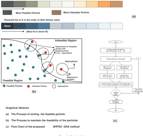
Graphical Abstract
(a) The Process of sorting the feasible particle
(b) The Process to maintain the feasibility of the particles
(c) Flow Chart of the proposed SHPSO -GSA method
(a)
(b)
(c)
Introduction
Introduction of PSO and GSA
Implementation and design of SHPSO -GSA Idea to propose new
Algorithm
Proposal of New SHPSO -GSA algorithm
Theortical Convergence and Parameter Setting
Benchmarking of the proposed algorithm over constrained
optimization problems ( CEC2006 )
and statistical testing
Benchmarking over Unconstrained optimization
problems ( CEC 2015) and
statistical testing
Results and Conclusions
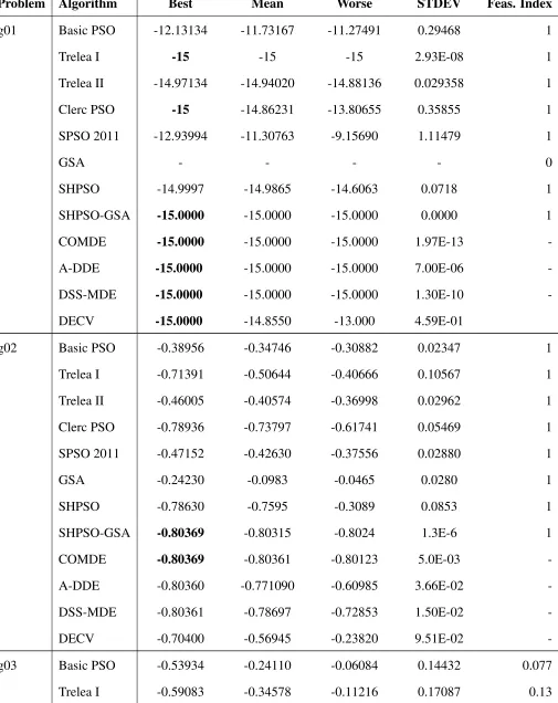
Table 7: Comparative results of objective function values
Problem Algorithm Best Mean Worse STDEV Feas. Index
g01 Basic PSO -12.13134 -11.73167 -11.27491 0.29468 1
Trelea I -15 -15 -15 2.93E-08 1
Trelea II -14.97134 -14.94020 -14.88136 0.029358 1
Clerc PSO -15 -14.86231 -13.80655 0.35855 1
SPSO 2011 -12.93994 -11.30763 -9.15690 1.11479 1
GSA - - - - 0
SHPSO -14.9997 -14.9865 -14.6063 0.0718 1
SHPSO-GSA -15.0000 -15.0000 -15.0000 0.0000 1
COMDE -15.0000 -15.0000 -15.0000 1.97E-13
-A-DDE -15.0000 -15.0000 -15.0000 7.00E-06
-DSS-MDE -15.0000 -15.0000 -15.0000 1.30E-10
-DECV -15.0000 -14.8550 -13.000 4.59E-01
g02 Basic PSO -0.38956 -0.34746 -0.30882 0.02347 1
Trelea I -0.71391 -0.50644 -0.40666 0.10567 1
Trelea II -0.46005 -0.40574 -0.36998 0.02962 1
Clerc PSO -0.78936 -0.73797 -0.61741 0.05469 1
SPSO 2011 -0.47152 -0.42630 -0.37556 0.02880 1
GSA -0.24230 -0.0983 -0.0465 0.0280 1
SHPSO -0.78630 -0.7595 -0.3089 0.0853 1
SHPSO-GSA -0.80369 -0.80315 -0.8024 1.3E-6 1
COMDE -0.80369 -0.80361 -0.80123 5.0E-03
-A-DDE -0.80360 -0.771090 -0.60985 3.66E-02
-DSS-MDE -0.80361 -0.78697 -0.72853 1.50E-02
-DECV -0.70400 -0.56945 -0.23820 9.51E-02
-g03 Basic PSO -0.53934 -0.24110 -0.06084 0.14432 0.077
Trelea I -0.59083 -0.34578 -0.11216 0.17087 0.13
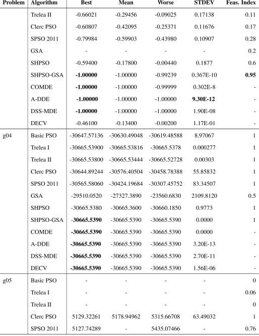
Table 7 –Continued from previous page
Problem Algorithm Best Mean Worse STDEV Feas. Index
Trelea II -0.66021 -0.29456 -0.09025 0.17138 0.11
Clerc PSO -0.60807 -0.42095 -0.25371 0.11676 0.17
SPSO 2011 -0.79984 -0.59903 -0.43980 0.10907 0.28
GSA - - - - 0.2
SHPSO -0.59400 -0.17800 -0.00440 0.1877 0.6
SHPSO-GSA -1.00000 -1.00000 -0.99239 0.367E-10 0.95
COMDE -1.00000 -1.00000 -0.99999 0.302E-8
-A-DDE -1.00000 -1.00000 -1.00000 9.30E-12
-DSS-MDE -1.00000 -1.00000 -1.00000 1.90E-08
-DECV -0.46100 -0.13400 -0.00200 1.17E-01
-g04 Basic PSO -30647.57136 -30630.49048 -30619.48588 8.97067 1
Trelea I -30665.53900 -30665.53816 -30665.5378 0.000277 1
Trelea II -30665.53800 -30665.53444 -30665.52728 0.00303 1
Clerc PSO -30644.89244 -30576.40504 -30458.78388 55.85832 1
SPSO 2011 -30565.58060 -30424.19684 -30307.45752 83.34507 1
GSA -29510.0520 -27327.3890 -23560.6830 2109.8120 0.5
SHPSO -30665.5380 -30665.3600 -30660.1850 0.9773 1
SHPSO-GSA -30665.5390 -30665.5390 -30665.5390 0.0000 1
COMDE -30665.5390 -30665.5390 -30665.5390 0.0000
-A-DDE -30665.5390 -30665.5390 -30665.5390 3.20E-13
-DSS-MDE -30665.5390 -30665.5390 -30665.5390 2.70E-11
-DECV -30665.5390 -30665.5390 -30665.5390 1.56E-06
-g05 Basic PSO - - - - 0
Trelea I - - - - 0.06
Trelea II - - - - 0
Clerc PSO 5129.32261 5178.94962 5315.66708 63.49032 1
Table 7 –Continued from previous page
Problem Algorithm Best Mean Worse STDEV Feas. Index
GSA - - - - 0
SHPSO - - - - 0.5
SHPSO-GSA 5126.4967 5126.4967 5126.4967 0.0000 1
COMDE 5126.4981 5126.4981 5126.4981 0.0000
-A-DDE 5126.4970 5126.4970 5126.4970 2.10E-11
-DSS-MDE 5126.4970 5126.4970 5126.4970 0.000
-DECV 5126.4970 5126.4970 5126.4970 0.000
-g06 Basic PSO -6933.28680 -6897.26958 -6855.47497 29.82939 1
Trelea I -6961.80842 -6961.79465 -6961.76673 0.013544 1
Trelea II -6960.29072 -6956.66901 -6952.08561 2.523567 1
Clerc PSO -6883.87603 -6464.55368 -5784.23680 371.61882 1
SPSO 2011 -6891.97980 -5935.52414 -4666.83552 743.4924772 1
GSA -3744.2747 2.7931E+05 1.0208E+06 2.4217E+05 0
SHPSO -6961.8136 -6961.8132 -6961.8090 0.0008 1
SHPSO-GSA -6961.8139 -6961.8139 -6961.8139 0.0000 1
COMDE -6961.8138 -6961.8138 -6961.8138 0.0000
-A-DDE -6961.8140 -6961.8140 -6961.8140 2.11E-12
-DSS-MDE -6961.8140 -6961.8140 -6961.8140 0.0000
-DECV -6961.8140 -6961.8140 -6961.8140 0.0000
-g07 Basic PSO 82.04177 121.49313 173.21687 29.27512 0.97933
Trelea I 25.61511 26.216681 27.01475 0.44408 1
Trelea II 38.51871 41.405807 44.83348 1.95376 1
Clerc PSO 24.61889 25.193279 26.54658 0.59327 1
SPSO 2011 41.01492 108.01448 320.67014 96.72589 1
GSA 850.4374 2103.3302 4824.1543 1076.3890 0.2
SHPSO 24.9019 25.1638 27.9587 0.5415 1
SHPSO-GSA 24.3062 24.3062 24.3062 0.0000 1
Table 7 –Continued from previous page
Problem Algorithm Best Mean Worse STDEV Feas. Index
COMDE 24.3062 24.3062 24.3062 4.7E-07
-A-DDE 24.3060 24.3060 24.3060 4.20E-05
-DSS-MDE 24.3060 24.3060 24.3060 7.50E-07
-DECV 24.3060 24.7940 29.5110 1.37E+00
-g08 Basic PSO -0.09582 -0.09582 -0.09582 3.44E-14 1
Trelea I -0.09582 -0.09582 -0.09582 1.38E-17 1
Trelea II -0.09582 -0.09582 -0.09582 1.50E-17 1
Clerc PSO -0.09582 -0.09582 -0.09582 1.61E-17 1
SPSO 2011 -0.09582 -0.09582 -0.09582 1.60E-17 1
GSA -0.09580 0.5679 53.5663 6.4742 0.7
SHPSO -0.09580 -0.0958 -0.0958 0.0000 1
SHPSO-GSA -0.09580 -0.09580 -0.09580 0.0000 1
COMDE -0.09580 -0.0958 -0.0958 9.00E-18
-A-DDE -0.09580 -0.0958 -0.0958 9.10E-10
-DSS-MDE -0.09580 -0.0958 -0.0958 4.00E-17
-DECV -0.09580 -0.0958 -0.0958 4.23E-17
-g09 Basic PSO 711.16899 730.88847 747.02641 11.59183 1
Trelea I 680.74916 680.86869 680.99542 0.072776 1
Trelea II 684.51697 686.22695 688.10022 1.218367 1
Clerc PSO 680.67590 680.74817 680.83062 0.044645 1
SPSO 2011 680.87510 689.21798 732.40846 15.15200 1
GSA 836.16420 1.4309E+06 9.5128E+06 2.2672E+06 0.8
SHPSO 680.64850 680.69560 680.7703 0.0234 1
SHPSO-GSA 680.63000 680.63000 680.63000 0.0000 1
COMDE 680.63001 680.63001 680.63001 4.071E-13
-A-DDE 680.63001 680.63001 680.63001 1.15E-10
-Table 7 –Continued from previous page
Problem Algorithm Best Mean Worse STDEV Feas. Index
DECV 680.63001 680.63001 680.63001 3.45E-07
-g10 Basic PSO 10785.19568 11901.53736 13316.83004 830.65975 0.8
Trelea I 7831.87690 8203.07587 8951.75208 318.29829 1
Trelea II 9184.23861 10081.46538 10707.05976 536.45609 0.9
Clerc PSO 7063.0057 7208.54728 7522.17599 151.91782 1
SPSO 2011 7702.34856 11559.18985 16060.10486 2948.23499 1
GSA - - - - 0.2
SHPSO 7331.9543 7590.6267 12288.9460 888.4462 1
SHPSO-GSA 7049.2480 7049.2480 7049.2480 0.0000 1
COMDE 7049.2480 7049.2480 7049.2480 1.5E-04
-A-DDE 7049.2480 7049.2480 7049.2480 3.23E-04
-DSS-MDE 7049.2480 7049.2490 7049.2550 1.40E-03
-DECV 7049.2480 7103.5480 7808.9800 1.48E+02
-g11 Basic PSO 0.75090 0.76917 0.82647 0.02183 0.1
Trelea I 0.75073 0.77771 0.82684 0.02708 0.37
Trelea II 0.75058 0.75904 0.78710 0.01103 0.21
Clerc PSO 0.75293 0.77908 0.82047 0.02635 0.59
SPSO 2011 0.75033 0.77466 0.88049 0.04422 0.68
GSA 0.84520 1.6221 4.5674 1.16550 0.9
SHPSO 0.75000 0.8220 0.9997 0.08270 1
SHPSO-GSA 0.74990 0.74990 0.74990 0.0000 1
COMDE 0.74991 0.74991 0.74991 0.0000
-A-DDE 0.75000 0.75000 0.75000 5.35E-15
-DSS-MDE 0.74991 0.74991 0.74991 0.0000
-DECV 0.75000 0.75000 0.75000 1.12E-16
-g12 Basic PSO -0.99999 -0.99998 -0.99996 1.15E-05 1
Trelea I -1.00000 -1.00000 -1.00000 0.00000 1
Table 7 –Continued from previous page
Problem Algorithm Best Mean Worse STDEV Feas. Index
Trelea II -1.00000 -1.00000 -1.00000 0.00000 1
Clerc PSO -1.00000 -1.00000 -1.00000 0.00000 1
SPSO 2011 -1.00000 -1.00000 -1.00000 0.00000 1
GSA -0.99990 -0.82040 -0.87030 0.00290 0.99
SHPSO -1.00000 -1.00000 -1.00000 0.00000 1
SHPSO-GSA -1.00000 -1.00000 -1.00000 0.00000 1
COMDE -1.00000 -1.00000 -1.00000 0.00000
-A-DDE -1.00000 -1.00000 -1.00000 4.10E-09
-DSS-MDE -1.00000 -1.00000 -1.00000 0.00000
-DECV -1.00000 -1.00000 -1.00000 0.00000
-g13 Basic PSO - - - - 0
Trelea I - - - - 0.07066
Trelea II - - - - 0
Clerc PSO 0.74535 - 0.99986 - 0.58
SPSO 2011 0.51468 - 1.76553 - 0.96
GSA - - - - 0.5
SHPSO - - - - 0.9
SHPSO-GSA 0.05390 0.05390 0.05390 0.00000 1
COMDE 0.05390 0.05390 0.05390 1.4E-17
-A-DDE 0.05390 0.07620 0.43880 1.00E-13
-DSS-MDE 0.05390 0.05390 0.05390 1.00E-13
-DECV 0.05970 0.38240 0.99900 2.68E-01
-g14 Basic PSO - - - - 0
Trelea I - - - - 0
Trelea II - - - - 0
Clerc PSO - - - - 0
Table 7 –Continued from previous page
Problem Algorithm Best Mean Worse STDEV Feas. Index
GSA - - - - 0.2
SHPSO - - - - 0.029
SHPSO-GSA -47.7649 -47.7649 -47.7649 0.0000 1
COMDE -47.7648 -47.7648 -47.7648 0.0000
-A-DDE -47.7648 -47.7641 -47.7640 9.0E-06
-DSS-MDE - - - -
-DECV -47.7648 -47.7225 -47.0365 1.62E-01
-g15 Basic PSO - - - - 0
Trelea I - - - - 0.00133
Trelea II - - - - 0
Clerc PSO 962.10129 963.84503 967.04043 1.57568 0.89133
SPSO 2011 961.82955 964.09145 969.87642 2.95027 1
GSA 963.95780 811.60760 983.46470 97.7669 0.1
SHPSO 967.09500 966.81230 969.91590 0.80730 0.3
SHPSO-GSA 961.71500 961.71500 961.71500 0.00000 1
COMDE 961.71500 961.71500 961.71500 0.00000
-A-DDE 961.71500 961.71500 961.71500 0.00000
-DSS-MDE - - - -
-DECV 961.71500 961.71500 961.7150 2.31E-01
-g16 Basic PSO -1.89386 -1.88638 -1.87975 0.00379 1
Trelea I -1.90515 -1.90515 -1.90515 2.73E-09 1
Trelea II -1.90493 -1.90482 -1.90468 8.09E-05 1
Clerc PSO -1.90515 -1.88138 -1.79158 0.0397 1
SPSO 2011 -1.80035 -1.63310 -1.45734 0.1115 1
GSA - - - - 0.1
SHPSO -1.90520 -1.90520 -1.90520 0.00000 1
SHPSO-GSA -1.90520 -1.90520 -1.90520 0.00000 1
Table 7 –Continued from previous page
Problem Algorithm Best Mean Worse STDEV Feas. Index
COMDE -1.90510 -1.90510 -1.90510 0.00000
-A-DDE -1.90510 -1.90510 -1.90510 0.00000
-DSS-MDE - - - -
-DECV -1.9051 -1.9051 -1.9051 1.10E-06
-g17 Basic PSO - - - - 0
Trelea I - - - - 0
Trelea II - - - - 0
Clerc PSO 8900.87142 8988.16628 9146.99254 87.12748 1
SPSO 2011 - - - - 0.28
GSA - - - - 0.1
SHPSO - - - - 0.5
SHPSO-GSA 8853.54019 8853.23453 8887.23422 0.0034 1
COMDE 8853.54002 8856.50010 8859.84000 1.35E-02
-A-DDE 8853.54002 8854.66400 8858.87400 1.43E+00
-DSS-MDE - - - -
-DECV 8853.5412 8919.9363 8938.5710 2.59E+01
-g18 Basic PSO - - - - 0
Trelea I -0.78433 -0.64646 -0.55436 0.068323 1
Trelea II -0.55439 -0.45036 -0.38724 0.054303 0.55
Clerc PSO -0.86285 -0.70750 -0.53972 0.106072 1
SPSO 2011 - - - - 0.56
GSA -0.29280 0.5234 193.3305 58.4214 0.33
SHPSO -0.64890 -0.6080 -0.1744 0.0846 1
SHPSO-GSA -0.86600 -0.86600 -0.86600 0.00000 1
COMDE -0.86600 -0.86600 -0.86600 0.00000
-A-DDE -0.86600 -0.86600 -0.86600 0.00000
-Table 7 –Continued from previous page
Problem Algorithm Best Mean Worse STDEV Feas. Index
DECV -0.86600 -0.85960 -0.67490 3.48E-02
-g19 Basic PSO 116.34307 149.73991 178.53261 16.00399 1
Trelea I 52.327558 56.735485 64.54874 3.759886 1
Trelea II 75.831398 85.461093 94.23523 5.437420 1
Clerc PSO 39.222218 43.781070 46.80910 2.678964 1
SPSO 2011 98.088985 131.92794 221.03201 32.37753 1
GSA 954.23940 18959.77900 41292.36700 8886.98110 0.8
SHPSO 40.56930 45.12000 92.89390 9.18240 1
SHPSO-GSA 32.65550 32.65550 32.65550 0.00000 1
COMDE 32.65550 32.6555 32.6555 1.41E-19
-A-DDE 32.65550 32.65800 32.66500 1.72E-03
-DSS-MDE - - - -
-DECV 32.65550 32.66050 32.78530 2.37E-02
-g21 Basic PSO - - - - 0
Trelea I - - - - 0
Trelea II - - - - 0
Clerc PSO - - - - 0
SPSO 2011 - - - - 0
GSA - - - - 0
SHPSO - - - - 0.2
SHPSO-GSA 193.7245 193.7245 193.7245 0.0000 1
COMDE 193.7245 193.7245 193.7245 1.39E-18
-A-DDE 193.7245 193.7245 193.7260 2.60E-04
-DSS-MDE - - - -
-DECV 193.7245 198.0905 324.7028 2.39E+01
-g23 Basic PSO - - - - 0
Trelea I - - - - 0
Table 7 –Continued from previous page
Problem Algorithm Best Mean Worse STDEV Feas. Index
Trelea II - - - - 0
Clerc PSO - - - - 0
SPSO 2011 - - - - 0.04
GSA - - - - 0
SHPSO - - - - 0.1
SHPSO-GSA -400.0551 -400.0547 -400.0546 0.0000 1
COMDE -400.0551 -399.4551 396.2345 1.91E-01
-A-DDE -400.0551 -391.4150 -367.4520 9.13E+00
-DSS-MDE - - - -
-DECV -400.0550 -392.0296 -342.5245 1.23E+01
-g24 Basic PSO -5.50801 -5.50800 -5.50799 5.27E-06 1
Trelea I -5.50801 -5.50801 -5.50801 7.02E-16 1
Trelea II -5.50801 -5.50801 -5.50801 7.02E-16 1
Clerc PSO -5.50801 -5.50801 -5.50801 7.02E-16 1
SPSO 2011 -5.50801 -5.50436 -5.48873 0.006172 1
GSA -5.42720 -3.70590 -1.20990 1.23290 0.8
SHPSO -5.50800 -5.50800 -5.50800 0.00000 1
SHPSO-GSA -5.50801 -5.50801 -5.50801 0.00100 1
COMDE -5.50801 -5.50801 -5.50801 0.0000
-A-DDE -5.50801 -5.50801 -5.50801 3.12E-14
-DSS-MDE - - - -
Table 11: Wilcoxon signed rank test results of single-problem analysis with a significance level ofα=0.05 for CEC 2006 problems
Pairwise Comparison of SHPSO-GSA Versus
Prob. Basic PSO Trelea I Trelea II Clerc PSO SPSO GSA SHPSO COMDE DSS-MDE DECV
g01 + + + + + + + 0 + 0
g02 + + + + + + + 0 + +
g03 + + + + + + + 0 + +
g04 + + + + + + + 0 + 0
g05 + + + 0 0 + 0 0 + +
g06 + + + + + + + 0 0 +
g07 + + + + − + + 0 0 +
g08 + + + + + + + 0 + +
g09 + + + + + + + 0 + +
g10 + + + + + + + 0 + 0
g11 − + − + + + + 0 + +
g12 + + + + + 0 0 + 0 ∗
g13 + + + + + 0 0 ∗ + ∗
g14 0 + 0 0 + 0 0 ∗ + ∗
g15 + + + 0 + 0 0 ∗ + ∗
g16 + + + + + 0 0 ∗ + ∗
g17 0 + 0 0 + 0 0 ∗ + ∗
g18 + + + + + 0 0 ∗ + ∗
g19 + + + + + 0 0 ∗ + ∗
g23 + + 0 0 + 0 0 ∗ + ∗
g24 + 0 + + + 0 0 ∗ ∗ ∗