The Quality of the Covariance Selection through
Detection Problem and AUC Bounds
Navid Tafaghodi Khajavi∗and Anthony Kuh
Department of Electrical Engineering, University of Hawaii, Honolulu, HI 96822, Email: {navidt, kuh}@hawaii.edu
* Correspondence: [email protected] Version November 15, 2017 submitted to MDPI
Abstract:This paper considers the problem of quantifying the quality of a model selection problem 1
for a graphical model. The model selection problem often uses a distance measure such as the 2
Kulback-Leibler (KL) distance to quantify the quality of the approximation between the original 3
distribution and the model distribution. We extend this work by formulating the problem as a 4
detection problem between the original distribution and the model distribution. In particular, we 5
focus on the covariance selection problem by Dempster, [1], and consider the cases where the 6
distributions are Gaussian distributions. Previous work showed that if the approximation model is a 7
tree, that the optimal tree that minimizes the KL divergence can be found by using the Chow-Liu 8
algorithm [2]. While the algorithm minimizes the KL divergence it does not minimize other measures 9
such as other divergences and the area under the curve (AUC). These measures all depend on the 10
eigenvalues of the correlation approximation measure (CAM). We find expressions for KL divergence, 11
log-likelihood ratio, and AUC as a function of the CAM. Easily computable upper and lower bounds 12
are also found for the AUC. The paper concludes by computing these measures for real and synthetic 13
simulation data. 14
Keywords: covariance selection; model approximation; detection problem; area under the curve; 15
information divergences 16
1. Introduction 17
Graphical models are useful tools for describing the geometric structure of networks in numerous 18
applications such as energy, social, sensor, biological, and transportation networks [3] that deal with 19
high dimensional data. Learning from these high dimensional data requires large computation power 20
which is not always available [4], [5]. The hardware limitation for different applications force us to 21
compromise between the accuracy of the learning algorithm and its time complexity by using the best 22
possible approximation algorithm given the constrained graph. In other words, the main concern is 23
to compromise between model complexity and its accuracy by choosing a simpler, yet informative 24
model. There are lots of approximation algorithms that are proposed for model selection to impose 25
structure given data. For the Gaussian distribution, the covariance selection problem is presented and 26
studied in [1] and [6]. 27
The ultimate purpose of the covariance selection problem is to reduce the computational 28
complexity in various applications. One of the special approximation models is the tree approximation 29
model. Tree approximation algorithms are among the algorithms that reduce the number of 30
computations to get quicker approximate solutions to a variety of problems. If a tree model is 31
used, then distributed estimation algorithms such as message passing algorithm [7] and the belief 32
propagation algorithm [8] can easily be applied and are guaranteed to converge to the maximum 33
likelihood solution. 34
There are algorithms in the literature such as the Chow-Liu minimum spanning tree (MST) [2], the 35
first order Markov chain approximation [9] and penalized likelihood methods such as LASSO [10] and 36
graphical LASSO [11] that can be used to approximate the correlation matrix and the inverse correlation 37
matrix with a more sparse graph representation while retaining good accuracy. The Chow-Liu MST 38
algorithm for Gaussian distribution is to find the optimal tree structure using a Kullback-Leibler 39
(KL) divergence cost function [1]. The Chow-Liu MST algorithm constructs a weighted graph by 40
computing pairwise mutual informations and then utilizes one of the MST algorithms such as the 41
Kruskal algorithm [12] or the Prim algorithm [13]. The first order Markov chain approximation uses a 42
regret cost function to output first order Markov chain structured graph [9] by utilizing a greedy type 43
algorithm. Penalized likelihood methods uses an L1-norm penalty term in order to sparsify the graph 44
representation and eliminate some edges. Recently, a tree approximation in a linear, underdetermined 45
model is proposed in [14] where the solution is based on expectation, maximization (EM) algorithm 46
combined with the Chow Liu algorithm. 47
Sparse modeling has many applications in distributed signal processing and machine learning 48
over graphs. One of its applications is for the electric power grid at the distribution level. Thesmart grid 49
is a promising solution that delivers reliable energy to consumers through the power grid when there 50
are uncertainties such as distributed renewable energy generation sources. Smart grid technologies 51
such as smart meters and communication links are added to the distribution grid in order to obtain the 52
high dimensional, real-time data and information and overcome uncertainties and unforeseen faults. 53
The future grid will incorporate distributed renewable energy generation such as solar photovoltaics 54
(PV), with these energy sources being highly correlated. Thus, modeling is an essential part for signal 55
processing and implementation of the smart grid. 56
We discuss the quality of the model selection problem, focusing on the Gaussian case, i.e. 57
covariance selection problem. We ask the following important question:“is the covariance approximation 58
of the covariance matrix for the Gaussian model a good approximation?"To answer this question, we need 59
to pick a closeness criterion which has to be coherent and general enough to handle a wide variety 60
of problems and also have asymptotic justification [15]. In many applications the Kullback-Leibler 61
(KL) divergence has been proposed as a closeness criterion between the original distribution and its 62
model approximation distribution [1] and [2]. Besides that, other closeness measures and divergences 63
are used for the model selection problem. One example is the use of reverse KL divergence as the 64
closeness criterion in variational methods to learn the desired approximation structure [16]. 65
In this paper we bring a different perspective to the model approximation problem by formulating 66
a general detection problem. The detection problem leads to calculation of the log-likelihood ratio test 67
(LLRT) statistic, the receiver operating characteristic (ROC) curve, the KL divergence and the reverse 68
KL divergence as well as the area under the curve (AUC) where the AUC is used as the accuracy 69
measure for the detection problem. The detection problem formulation gives us a broader view as well 70
as looking at different approaches of determining whether a particular model is a good approximation 71
or not. More specifically, the AUC gives us additional incite about any approximation since it is a way 72
to formalize the model approximation problem. For Gaussian data, the LLRT statistic simplifies to 73
an indefinite quadratic form. A key quantity that we define is the correlation approximation matrix 74
(CAM) as the product of the original correlation matrix and the inverse of the model approximation 75
correlation matrix. For Gaussian data this matrix contains all the information needed to compute the 76
information divergences, the ROC curve and the area under this curve, i.e. the AUC. We also show the 77
relationship between the CAM, the AUC and the Jeffreys divergence [17], the KL divergence and the 78
reverse KL divergence. We present an analytical expression to compute the AUC for a given CAM that 79
can be efficiently evaluated numerically. We show the relation between the AUC, the KL divergence, 80
the LLRT statistics and the ROC curve. We also present analytical upper and lower bounds for the 81
AUC which are only depend on eigenvalues of the CAM. Throughout the discussion section, we pick 82
the tree approximation model as a well-known subset of all graphical models. The tree approximations 83
is considered since they are widely used in literature and it is much simpler performing inference 84
and estimation on trees rather than graphs that have cycles or loops. We perform simulations over 85
indicate that 1−AUC is decreasing exponentially as the number of nodes of the graph increases which 87
is consistent with analytical results obtained from the AUC upper and lower bounds. 88
The rest of this paper is organized as follows. In section2we give a general framework for the 89
detection problem and the corresponding sufficient test statistic, the log-likelihood ratio test. Moreover, 90
the sufficient test statistic for Gaussian data as well as its distribution under both hypotheses are also 91
presented in this section. The ROC curve and the AUC definition as well as analytical expression for 92
the AUC are given in section3. Section4provides analytical lower and upper bounds for the AUC. 93
The lower bound for the AUC uses the Chernoff bound and is a function of the CAM eigenvalues. 94
The upper bound is obtained by finding a parametric relationship between the AUC and the KL and 95
reverse KL divergences. Moreover, Section5presents the tree approximation model and provides 96
some simulations over synthetic examples as well as real solar data examples and investigates quality 97
of the tree approximation based on the numerically evaluated AUC and also its analytical upper and 98
lower bounds. Finally, Section6summarizes results of this paper. 99
2. Detection Problem Framework 100
In this section, we present a framework to quantify the quality of a model selection problem. 101
More specifically, we formulate a detection problem to distinguish between the covariance matrix of 102
a multivariate normal distribution and an approximation of the aforementioned covariance matrix 103
based on the given model. 104
2.1. Model selection problem 105
We want to approximate a multivariate distribution by the product of lower order component 106
distributions [18]. Let random vectorX∈Rn, have a distribution with parameterΘ, i.e.X∼ f X(x). 107
We want to approximate the random vectorX, with another random vector associated with the desired 108
model1. Let the model random vectorXM∈Rnhave a distribution with parameterΘM, associated
109
with the desired model, i.e. X∼ fXM(x). Also, letG = (V,EM)be the graph representation of the
110
model random vectorXMwhere setsVandEMare the set of all vertices and the set of all edges of the
111
graph representing ofXM, respectively. Moreover,EM⊆ψwhereψis the set of all edges of complete 112
graph with vertex setV. 113
Remark:Covariance selection is presented in [1]. Moreover, tree model as a special case for the model 114
selection problem is discussed in subsection5.1. 115
2.2. General detection framework 116
The model selection problem is extensively studied in the literature [1]. In many state of the art 117
works, minimizing the KL divergence between two distributions or the maximum likelihood criterion 118
are proposed in order to quantify the quality of the model approximation. A different way to look 119
at the problem of quantifying the quality of the model approximation algorithm is to formulate the 120
problem as a detection problem [19]. Given the set of data in the detection problem, the goal is to 121
distinguish between two hypotheses, the null hypothesisandthe alternative hypothesis. To set up a 122
detection problem, we need to define these two hypotheses for the model selection problem as follow 123
- The null hypothesis,H0: The hypothesis that data is generated using the known distribution, 124
- The alternative hypothesis, H1: The hypothesis that data is generated using the model 125
approximation distribution. 126
Given the set up for the null hypothesis and the alternative hypothesis, we need to define a test statistic to quantify the detection problem. The likelihood ratio test (the Neyman-Pearson (NP) Lemma [20]) is the most powerful test statistic where we first define the log-likelihood ratio test (LLRT) as
l(x) =log fX(x|H1) fX(x|H0)
=log fXM(x)
fX(x)
where fX(x|H0)is the distribution of random vectorXunder the null hypothesis whilefX(x|H1)is 127
the distribution of random vectorXunder the alternative hypothesis. 128
We then definethe false-alarm probabilityandthe detection probabilityby comparing the LLRT statistic 129
under each hypothesis with a given threshold,τ, and computing the following probabilities 130
- The false-alarm probability,P0(τ), under the null hypothesis,H0:P0(τ) =Pr(L(X)≥τ|H0), 131
- The detection probability,P1(τ), under the alternative hypothesis,H1:P1(τ) =Pr(L(X)≥τ|H1), 132
where random variableL(X)is the LLRT statistic random variable. 133
The most powerful test is defined by setting the false-alarm rateP0(τ) =P¯0and then computing the 134
threshold valueτ0such that Pr(L(X)≥τ0|H0) =P¯0. 135
Definition 1. The KL divergence between two multivariate continuous distributions p(X)and q(X)is defined as
D pX(x)||qX(x)
= Z
X pX(x)log
pX(x) qX(x) dx
whereX is the feasible set.
136
Throughout this paper we may use other notations such as the KL divergence between two 137
random variable or the KL divergence between two covariance matrices for zero-mean Gaussian 138
distribution case in order to present the KL divergence between two distributions. 139
Proposition 1. Expectation of the LLRT statistic under each hypothesis is 140
- E(L(X)|H0) =−D(fX(x|H0)||fX(x|H1)) =−D(fX(x)||fXM(x)), 141
- E(L(X)|H1) =D(fX(x|H1)||fX(x|H0)) =D(fXM(x)||fX(x)). 142
Proof. Proof is based on the KL divergence definition.
143
Remark: Relationship between the NP lemma and the KL divergence is previously stated in [21] 144
with the similar straightforward calculation, where the LLRT statistic loses power when the wrong 145
distribution is used instead of the true distribution for one of these hypotheses. 146
In a regular detection problem framework, the NP decision rule is to accept the hypothesisH1if 147
the LLRT statistic,l(x), exceeds a critical value, and reject it otherwise. Moreover, the critical value is 148
set based on the rejection probability of the hypothesisH0, i.e. false-alarm probability. Note that, we 149
pursue a different goal in the approximation problem scenario. We approximate a model distribution, 150
fXM(x), as close as possible to the given distribution,fX(x). The closeness criterion is based on the 151
modified detection problem framework where we compute the LLRT statistic and compare it with a 152
threshold. In an ideal case where there is no approximation error, the detection probability must be 153
equal to the false-alarm probability for the optimal detector at all possible thresholds, i.e. the receiver 154
operating characteristic (ROC) curve [22] that represents best detectors for all threshold values should 155
be a line of slope 1 passing through the origin. 156
In the next, we assume that the random vectorXhas zero-mean Gaussian distribution. Thus, the 157
covariance matrix of the random vectorXis the parameter of interest in the model selection problem, 158
2.3. Multivariate Gaussian distribution 160
Let random vector X ∈ Rn, have a zero-mean jointly Gaussian distribution with covariance matrixΣX, i.e. X ∼ N(0,ΣX)where the covariance matrixΣXis positive-definite,ΣX 0. In this paper, the null hypothesis,H0, is the hypothesis that the parameter of interest is known and is equal toΣX while the alternative hypothesis,H1, is the hypothesis that the random vectorXis replaced by the model random vectorXM. In this scenario, the model random vectorXM has a zero-mean jointly Gaussian distribution (the model approximation distribution) with covariance matrixΣXM, i.e.XM ∼ N(0,ΣXM)where the covariance matrixΣXM is also positive-definite,ΣXM 0. Thus, the LLRT statistic for the jointly Gaussian random vectors,XandXM, is simplified as
l(x) =logN(0,ΣXM)
N(0,ΣX)
=−c+k(x) (1)
wherec=−1
2log(|ΣXΣX−1M|)is a constant andk(x) =x
TKxwhereK= 1 2(Σ
−1 X −Σ
−1
XM)is an indefinite 161
matrix with both positive and negative eigenvalues. 162
We define the correlation approximation matrix (CAM) associated with the covariance selection 163
problem and dissimilarity parameters of the CAM as follows. 164
Definition 2. Correlation approximation matrix.The CAM for the covariance selection problem is defined 165
as∆,ΣXΣ−XM1 whereΣXM is the model covariance matrix. 166
Definition 3. Dissimilarity parameters for covariance selection problem.Letαi ,λi+λ−i 1−2for 167
i∈ {1, . . . ,n}be dissimilarity parameters of the CAM correspond to the covariance selection problem where 168
λi >0for i∈ {1, . . . ,n}are eigenvalues of the CAM.
169
Remark: The CAM is a positive definite matrix. Moreover, eigenvalues of the CAM contains all 170
information necessary to compute cost functions associated with the model selection problem. 171
Theorem 1. Covariance Selection [1]. Given a multivariate Gaussian distribution with covariance matrix 172
ΣX 0, fX(x), and a modelM, there exists a unique approximated multivariate Gaussian distribution with 173
covariance matrixΣXM 0, fXM(x), that minimize the KL divergence,D(fX(x)||fXM(x))and satisfies the 174
covariance selection rules, i.e. the model covariance matrix satisfies the following covariance selection rules 175
- ΣXM(i,i) =ΣX(i,i), ∀i∈ V 176
- ΣXM(i,j) =ΣX(i,j), ∀(i,j)∈ EM 177
- Σ−X1
M(i,j) =0, ∀(i,j)∈ E c
M
178
where the setEc
M=ψ− EMrepresents the complement of the setEM.
179
Proof. Proof for Gaussian distributions is given in Dempster 1972 paper [1]. 180
Remark:Using the CAM definition, the constantccan be written asc=−12log(|∆|). Moreover, given 181
any covariance matrix and its model covariance matrix satisfying theorem1, we havetr(∆) =n. Thus, 182
from the result in theorem1and the definition of KL divergence for jointly Gaussian distributions, we 183
concludec=D(fX(x)||fXM(x)). 184
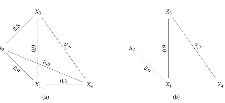
2.4. Covariance selection example 185
X1 X2
X3
X4 0.9
0.8
0.7
0.9
0.3
0.6
(a)
X1 X2
X3
X4 0.9
0.9
0.7
(b)
Figure 1.(a) The complete graph; (b) The tree approximation of the complete graph.
nonadjacent nodes is the multiplication of all correlations on the unique path that connects those nodes. The correlation matrix for each graph is
ΣX=
1 0.9 0.9 0.6
0.9 1 0.8 0.3
0.9 0.8 1 0.7
0.6 0.3 0.7 1
and
ΣXT =
1 0.9 0.9 0.63
0.9 1 0.81 0.567
0.9 0.81 1 0.7
0.63 0.567 0.7 1
.
The CAM for the above example is
∆=
1 0 0.0412 −0.0588
0.0474 1 0.3042 −0.5098
0.0474 −0.0526 1 0
0.9789 −1.2632 0.1421 1
.
The CAM contains all information about the tree approximation2. Here we assume cases that Gaussian 186
random variables have finite, nonzero variances. 187
Remark:Without loss of generality, throughout this paper we are working with normalized correlation 188
matrices, i.e. the diagonal elements of the correlation matrices are normalized to be equal to one. 189
2.5. Distribution of the LLRT statistic 190
The random vectorXhas Gaussian distribution under both hypothesesH0andH1. Thus under both hypotheses, the real random variable,K(X) =XTKXhas a generalized chi-squared distribution, i.e. the random variable,K(X), is equal to a weighted sum of chi-squared random variables with both positive and negative weights under both hypotheses. Let us defineW = Σ−12
X XunderH0 andZ = Σ−12
XMXunderH1, whereΣ
1 2
XandΣ
1 2
XM are the square root of covariance matricesΣX and
2 Dissimilarity parametersα
ΣXM, respectively. Then let random vectorsW ∼ N(0,I)andZ∼ N(0,I)have zero-mean Gaussian distributions with the same covariance matrices,I, whereIis the identity matrix of dimensionn. Note that, the CAM is a positive definite matrix withλi >0 where 1≤i≤n. Thus, the random variable K(X), under both hypothesesH0andH1can be written as:
K0(X),K(X)|H0= 1 2
n
∑
i=1
(1−λi)Wi2
and
K1(X),K(X)|H1= 1 2
n
∑
i=1
(λ−i 1−1)Zi2
respectively, where random variables Wi and Zi, are the i-th element of random vectors W and Z, respectively. Moreover, random variablesWi2andZi2, follow the first order central chi-squared distribution. Note that, similarly random variableL(X),−c+K(X)is defined under each hypothesis as
L0,L(X)|H0=−c+K0(X) and
L1,L(X)|H1=−c+K1(X).
Remark:As a simple consequence of the covariance selection theorem, the summation of weights for 191
the generalized chi-squared random variable, the expectation ofK(X), is zero under the hypothesis 192
H0, i.e. E(K0(X)) = 12∑ni=1(1−λi) =0 [1], and this summation is positive under the hypothesisH1, 193
i.e. E(K1(X)) = 12∑ni=1(λ −1
i −1)≥0. 194
3. The ROC Curve and the AUC Computation 195
3.1. The receiver operating characteristic curve 196
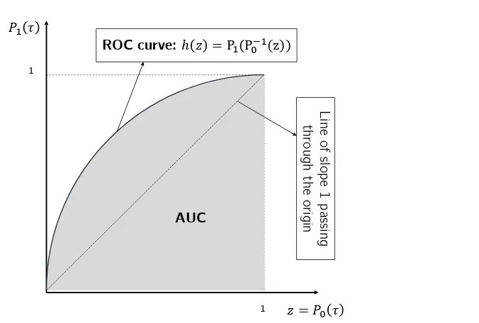
The receiver operating characteristic (ROC) curve is the parametric curve where the detection 197
probability is plotted versus the false-alarm probability for all thresholds, i.e. each point on the ROC 198
curve represents a pair of(P0(τ),P1(τ)) for a given thresholdτ. Setz = P0(τ)andη = P1(τ), the 199
ROC curve isη=h(z). IfP0(τ)has an inverse function, then the ROC curve ish(z) =P1(P0−1(z)). In 200
general, the ROC curve,h(z), has the following properties [22] 201
- h(z)is concave and increasing, 202
- h0(z)is positive and decreasing, 203
- R1
0 h
0(z)dz≤1.
204
Note that, for the ROC curve, the slope of the tangent line at a given threshold, h0(z), gives the 205
likelihood ratio for the value of the test. 206
Remark:For the ROC curve for our Gaussian random vectors we haveh0(z)is positive, continuous and decreasing in interval[0, 1]with right continuity at 0 and left continuity at 1. Moreover,
Z 1
0 h
0(z)dz=1
sinceh(0) =0 andh(1) =1. 207
Definition 4. Let fL0(l)and fL1(l)be the probability density function (PDF) of the random variables L0and 208
L1, respectively.
AUC
1 1
𝑧 = 𝑃0 𝜏
𝑃1 𝜏
ROC curve: ℎ 𝑧 = P1(P0−1(z))
L
ine
of
s
lope
1 pas
sing
throu
gh
t
he
origin
Figure 2.The ROC curve and the area under the ROC curve. Each point on the ROC curve indicates a detector with given detection and false-alarm probabilities.
Lemma 1. Given the ROC curve, h(z), we can compute following KL divergences
D fL1(l)||fL0(l)
=−
Z 1
0 log h 0(z)
dz. and
D fL0(l)||fL1(l)
=−
Z 1
0 h 0
(z)log h0(z)
dz
(∗)
= −
Z 1
0 log
d h−1(η) dη
dη
where (*) holds if the ROC curve,η=h(z), has an inverse function. 210
Proof. These results are consequence of the Radon-Nikodým theorem [23]. Simple, alternative calculus 211
based proofs are given in appendixA.
212
3.2. Area under the curve 213
As discussed previously we examine the ROC with a goal that the model approximation results 214
with the ROC being a line of slope 1 passing through the origin. This is in contrast to the conventional 215
detection problem where we want to distinguish between the two hypotheses and ideally have an 216
ROC that is a unit step function. Area under the curve (AUC) is defined as the integral of the ROC 217
curve (figure2) and is a measure of accuracy in decision problems. 218
Definition 5. The area under the ROC cure (AUC) is defined as
AUC= Z 1
0 h
(z)d z=
Z 1
0 P1
(τ)dP0(τ) (2)
whereτis the detection problem threshold.
Remark: The AUC is a measure of accuracy for the detection problem and1/2 ≤ AUC≤ 1. Note
220
that, in conventional decision problems, the AUC is desired to be as close as possible to 1 while in 221
approximation problem presented here we want the AUC to be close to1/2. 222
Theorem 2. Statistical property of AUC [24].The AUC for the LLRT statistic is AUC=Pr(L1>L0).
223
Corollary 1. From theorem2, when PDFs for the LLRT statistic under both hypotheses exist, we can compute the AUC as
AUC= Z ∞
0 fL1(l) ? fL0(l)dl (3)
where fL1(l) ? fL0(l),R−∞∞fL1(τ)fL0(l+τ)dl is the cross-correlation between fL1(l)and fL0(l).
224
Proof. A proof based on the definition of the AUC (2), is given in [25]. 225
Let us define the difference LLRT statistic random variable asL∆=L1−L0. Then, we get AUC=Pr(L∆>0)
=1−FL∆(0)
whereFL∆(l)is the cumulative distribution function (CDF) for random variableL∆. 226
The two conditional random variablesL0andL1are independent3. Thus, the cross-correlation between the corresponding two distributions is the distribution of the difference LLRT statistic,L∆. We can write the random variableL∆as
L∆=−c+K1(X)−(−c+K0(X))
=K1(X)−K0(X).
Replacing the definition forK0(X)andK1(X), we have
L∆= 1 2
n
∑
i=1
(λ−i 1−1)Z2i −1 2
n
∑
i=1
(1−λi)Wi2.
We can rewrite the difference LLRT statistic,L∆, in an indefinite quadratic form as
L∆= 1 2V
T(Λ−I)V
where
V=
W Z
and
Λ=
λ1
. .. 0
λn λ−11
0 . ..
λ−n1
.
3.3. Generalized Asymmetric Laplace distribution 227
The difference LLRT statistic random variable,L∆, follows the generalized asymmetric Laplace (GAL) distribution4[26]. For a giveniwherei∈ {1, . . . ,n}, we define random variableL∆i as
L∆i = λi−1
2 W
2 i −
1−λ−i 1
2 Z
2
i. (4)
Then, difference LLRT statistic random variable,L∆, can be written as
L∆= n
∑
i=1 L∆i
whereL∆i’s are independent and have GAL distributions at position 0 with meanαi/2and PDF [26]
fL∆
i(l) =
e2l
π√αiK0
r
α−i 1+1 4 |l|
!
, l6=0 (5)
whereK0(−)is the modified Bessel function of second kind [27]. The moment generating function (MGF) for this distribution is
ML∆
i(t) =
1
p
1−αit−αit2
for allt’s that satisfies 1−αit−αit2 >0. From (4), the MGF derivation for the GAL distribution is 228
straightforward and is the multiplication of two MGFs for the chi-squared distribution. 229
The distribution of the difference LLRT statistic random variable,L∆, is fL∆(l) = n
∗
i=1fL∆i(l)
where
∗
ni=1is the notation we use for convolution ofnfunctions together. Note that, although the distribution of random variablesL∆i’s in (5) has discontinuity atl =0, the distribution of random variableL∆is continuous if there are at least two distribution with non-zero parameters,αi’s, in the aforementioned convolution. Moreover, the MGF for fL∆(l)can be computed by multiplying MGFs forL∆i asML∆(t) = n
∏
i=1 ML∆
i(t) (6)
for allt’s in the intersection of all domains ofML∆i(t). The smallest of such intersections is−1<t<0. 230
3.4. Analytical expression for AUC 231
To compute the CDF of random variableL∆, we need to evaluate a multi-dimensional integral of jointly Gaussian distributions [28] or we need to approximate this CDF [29]. More efficiently, as discussed in [30] for the real valued case, the CDF of the random variableL∆can be expressed as a single-dimensional integral of a complex function5in the following form
FL∆(l) = 1 2π
Z ∞
−∞
e2l(jω+β)
jω+β
1
q
|I+12(Λ−I)(jω+β)|
dω
whereβ>0 is chosen such that matrixI+ β2(Λ−I), is positive definite and simplifies the evaluation 232
of the multivariate Gaussian integral [30]. 233
Special case:WhenΛ=I, i.e. the given covariance obeys the model structure, then
AUC=1−FL∆(0) =1− 1
2π Z ∞
−∞ 1 jω+β =
1 2
forβ>0 and is also independent of the value of the parameterβ. 234
Picking an appropriate value for the parameterβ6, the AUC can be numerically computed by evaluating the following one dimension complex integral
AUC=1− 1
2π Z ∞
−∞ 1 jω+β
1
q
|I+12(Λ−I)(jω+β)|
dω.
Furthermore, sinceΛ0, choosingβ=2 and changing variable asν=ω/2, we have
AUC=1− 1
2π Z ∞
−∞ 1 jν+1
1
p
|Λ+jν(Λ−I)| dν. (7)
Moreover,|Λ+jν(Λ−I)|=∏i=p 1(1+αiν2−jαiν). This equation shows that the AUC only depends 235
onαi’s. 236
Remark:Since the AUC integral in (7) can not be evaluated in closed form, it can not be used directly 237
in obtaining model selection algorithms. Numerical evaluation of the AUC using the one dimensional 238
complex integral (7) is very efficient and fast comparing to numerical evaluation of a multi-dimensional 239
integral of jointly Gaussian CDF. 240
4. Analytical Bounds for the AUC 241
As in the previous section we present an analytical expression for the AUC, in this section, we 242
presents analytical lower and upper bounds for the AUC. These bounds will give us insight on how 243
the AUC behave. 244
4.1. Lower bound for the AUC (Chernoff bound application) 245
Given the MGF for the difference LLRT statistic distribution (6), we can apply the Chernoff bound 246
[31] to find a lower bound for the AUC or upper bound for the CDF of the difference LLRT statistic 247
random variable,L∆, evaluated at zero). 248
5 This is the transform to the frequency domain for an arbitraryβ.
6 The parameterβis picked such thatI+β
Proposition 2. Lower bound for the AUC is
Pr(L∆>0)≥max
1 2, 1−e
−12∑n i=1log(1+
αi
4)
(8)
Proof. One-half is a trivial lower bound for AUC. To achieve a non-trivial lower bound, we apply Chernoff bound [31] as follow
Pr(L∆<0)≤inf
t ML∆(t).
To complete the proof we need to solve the right-hand-side (RHS) optimization problem. Step 1:First derivatives ofML∆(t)is
d
d tML∆(t) =ML∆(t) 1 2
n
∑
i=1
λi−1 1−(λi−1)t
+ λ
−1 i −1 1−(λ−i 1−1)t
!
=ML∆(t)(1+2t)
n
∑
i=1
αi
2(1−αit−αit2).
Clearly, first derivative is zero fort=−1/2which is in the feasible domain of the MGF for the difference
LLRT statistic. Note that, the smallest feasible domain is−1<t<0. Step 2:Second derivatives ofML∆(t)is
d2
d t2ML∆(t) =
ML∆(t) 1 4
n
∑
i=1
λi−1 1−(λi−1)t+
λ−i 1−1 1−(λ−i 1−1)t
!2
+
ML∆(t) 1 4
n
∑
i=1
(λi−1)2 (1−(λi−1)t)2
+ (λ
−1 i −1)2 (1−(λ−i 1−1)t)2
!
.
Therefore, we conclude that the second derivative is positive and thus the optimal solution to the RHS optimization problem is att=−12. Replacing that in the definition of the moment generation function which results in the following bound
Pr(L∆≤0)< n
∏
i=1 2
√
4+αi
which can be written as
Pr(L∆>0)≥1−
n
∏
i=1 2
√
4+αi
which completes the proof.
249
4.2. Upper Bound for the AUC 250
In this section, we present a parametric upper bound for the AUC, but first, we need to present 251
the following results. 252
Lemma 2. Invariance property of the KL divergence for the LLRT statistic.We have
and
D(fL0(l)||fL1(l))≤ D(fX(x|H0)||fX(x|H1)).
Proof. This lemma is an special case of the invariance property of the KL divergence [32]. By picking 253
appropriate measurable mapping, here appropriate quadratic function for each equation of the above 254
equations, we conclude the lemma.
255
AUC
1
KL
Div
erg
en
ce
0.5
AUC Lo
wer
Bou
nd
AUC U
pp
er
Bou
nd
Possible
Feasible
Region
B
oun
da
ry
cu
rve
for
possi
bl
e
fe
asi
bl
e
re
gi
on
cor
re
spon
ds
to
the
opt
im
al
ROC
cu
rve
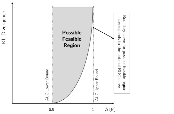
Figure 3.Possible feasible region for the AUC and the Kl divergence pair for all possible detectors or equivalently all possible ROC curves (the KL divergence is between the LLRT statistics under different hypotheses, i.e.D(fL0(l)||fL1(l))orD(fL1(l)||fL0(l)).)
Definition 6. Feasible Region.The AUC and the KL divergence pair is lying in the feasible region (figure3) 256
for all possible detectors (ROC curves), i.e. no detector with the AUC and the KL divergence pair lie outside the 257
feasible region7. 258
Theorem 3. Possible feasible region for the AUC and the KL divergence.Given the ROC curve, the parametric possible feasible region as shown in figure3can be expressed using the positive parameter a>0as
Pr(L∆>0) = 1 1−e−a −
1 a and
D∗l ≥log(a) + a
ea−1 −1−log(1−e
−a)
where
Dl∗=min
D(fL1(l)||fL0(l)),D(fL0(l)||fL1(l)) .
Proof. Proof is given in the appendixB.
259
Theorem3formulates the relationship between the AUC and the KL divergence.The results of this 260
theorem is generally true for any LLRT statistic. Theorem3states that for any valid ROC corresponds to 261
a detector, the pair of AUC and KL divergencemustlie in the possible feasible region (figure3), i.e. 262
outside of this region is infeasible. This possible feasible region results in the general upper bound for 263
AUC. 264
Since computing the distribution of the LLRT statistics is not straight forward in most cases, 265
proposition3, relaxes the Theorem3by bounding the KL divergence between the LLRT statistics using 266
the the invariance property of KL divergence for the LLRT statistic (lemma2). 267
Proposition 3. The parametric upper bound for AUC is
Pr(L∆>0) = 1 1−e−a −
1 a and
D∗≥log(a) + a
ea−1 −1−log(1−e
−a)
where a>0is a positive parameter and
D∗=min{ D(fX(x|H1)||fX(x|H0)), (9)
D(fX(x|H0)||fX(x|H1))}.
Proof. Proof is based on the lemma2and the possible feasible region presented in the theorem3. From the lemma2, we have
D∗l ≤ D∗.
Then, using the result in the theorem3, we get the parametric upper bound. 268
4.3. Asymptotic behavior for AUC bounds 269
Proposition 4. Asymptotic behavior of the lower bound.We have Pr(L∆>0)≥1−e−n(1−1n∑ni=1(1+
αi
8)−1).
Proof. Applying the inequality
2x
2+x <log(1+x)
forx>0, we achieve the result.
270
Proposition 5. Asymptotic behavior of the upper bound.The parametric upper bound for AUC has the following asymptotic behavior
Pr(L∆>0)≤1−e−D∗−1 whereD∗is given in(9).
271
Proof. Proof is as follows.
−log(1−Pr(L∆>0)) =−log
1 ea−1+
1 a
≤log(a)
Applying the exponential function to both sides of the above inequality we conclude the upper bound. 272
273
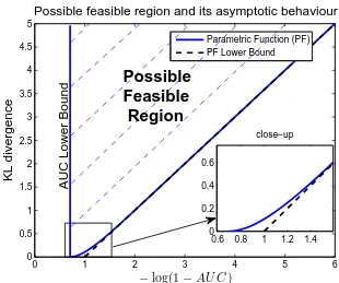
Figure4shows the possible feasible region and the asymptotic behavior log-scale. As it is shown 274
in this figure, the parametric upper bound can be approximated with a straight line especially for large 275
values of the parametera(the result in proposition5). Also, figure5shows the possible feasible region 276
and the asymptotic behavior in regular-scale. 277
0 1 2 3 4 5 6
0 0.5 1 1.5 2 2.5 3 3.5 4 4.5 5
−
log(1
−
AU C
)
KL divergence
Possible feasible region and its asymptotic behaviour
0.6 0.8 1 1.2 1.4 0
0.2 0.4 0.6
close−up
AUC Lower Bound
Parametric Function (PF) PF Lower Bound
Possible
Feasible
Region
Figure 4. Log-scale of the possible feasible region and its asymptotic behavior (linear line) for the AUC and the KL divergence pair for all possible detectors or equivalently all possible ROC curves (the KL divergence is between the LLRT statistics under different hypotheses, i.e.D(fL1(l)||fL0(l))or
D(fL0(l)||fL1(l)).) Close-up part shows the non-linear behavior of the possible feasible region around
one.
5. Examples and Simulation Results 278
In this section, we consider some examples of covariance matrices for Gaussian random vectorX. 279
We pick the tree structure as the graphical model corresponds to the covariance selection problem. In 280
our simulations, we compare the numerically evaluated AUC and its lower and upper bounds and 281
discuss their asymptotic behavior as the dimension of the graphical model,n, increases. 282
5.1. Tree approximation model 283
The maximum order of the lower order distributions in tree approximation problem is two, i.e. no more than pairs of variables. LetXT ∼ N(0,ΣXT)have the graph representationGT = (V,ET) whereET ⊆ ψis a set of edges that represents a tree structure. LetXr ∼ N(0,ΣXr)have the graph representationGr = (V,Er)whereEr ⊆ ET is the set of all edges in the graph ofXr. The joint PDF for elements of random vectorXrcan be represented by joint PDFs of two variables and marginal PDFs in the following convenient form
fXr(xr) =
∏
(u,v)∈Er
fXu,Xv(xu,xv) fXu(xu)fXv(xv)u
∏
∈V0.4 0.5 0.6 0.7 0.8 0.9 1 1.1 0
1 2 3 4 5 6
AUC
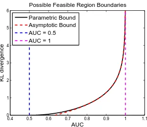
KL divergence
Possible Feasible Region Boundaries
Parametric Bound
Asymptotic Bound
AUC = 0.5
AUC = 1
Figure 5.The possible feasible region boundaries and its asymptotic behavior for the AUC and the KL divergence pair for all possible detectors or equivalently all possible ROC curves (the KL divergence is between the LLRT statistics under different hypotheses, i.e.D(fL0(l)||fL1(l))orD(fL1(l)||fL0(l)).).
Using equation (10) we can then easily construct a tree using iterative algorithms (such as the Chow-Liu algorithm [2] combined with the Kruskal [12] algorithm or the Prim [13] algorithm) by adding edges one at a time [34]. Consider the sequence of random vectors Xr with 0 ≤ r ≤ |ET|, whereXr is recursively generated by augmenting a new edge,(i,j)∈ Er, to the graph representation ofXr−1. For the special case of Gaussian distributions,ΣXr has the following recursive formulation [34]
Σ−1 Xr =Σ
−1 Xr−1+Σ
†
i,j−Σ†i −Σ†j , ∀0≤r≤ |ET|
whereΣ†i,j = [ei ej]Σ−i,j1[ei ej]T andΣ†i =eiΣi−1eTi whereeiis a unitary vector with 1 at thei-th place 284
andΣi,jandΣiare the 2-by-2 and 1-by-1 principle sub-matrices ofΣX, with initial stepΣX0=diag(ΣX)
285
wherediag(ΣX)represents a diagonal matrix with diagonal elements ofΣX. 286
Remark:For all 0≤r≤ |ET|, we have
287
1. tr(ΣXr) =tr(ΣX) 288
2. tr(ΣXΣ−X1r) =n. 289
3. D(fX(x)||fXr(x)) =−12log(|ΣXΣ−Xr1|) 290
4. |ΣX| ≤. . .≤ |ΣXr| ≤. . .≤ |ΣX0|=|diag(ΣX)| 291
5. H(X)≤. . .≤H(Xr)≤. . .≤H(X0). 292
Tree approximation models are interesting to study since there are algorithms such as Chow-Liu 293
[2] combined by the Kruskal [12] or the Prim’s [13] that efficiently compute the model covariance 294
5.2. Toeplitz example 296
Here, we assume that the covariance matrixΣXhas a Toeplitz structure with ones on the diagonal elements and the correlation coefficientρ>−(n−11)as off diagonal elements
ΣX=
1 ρ . . . ρ
ρ . .. ... ... ..
. . .. ... ρ ρ . . . ρ 1
.
For the tree structure model, all possible tree structured distributions satisfying (10) have the same 297
KL divergence to the original graph, i.e.D(fX(x)||fXT(x))is constant for all possible connected tree 298
approximation model for this example. The reason is that all the weights computed by the Chow-Liu 299
algorithm to construct the weighted graph associated with this problem are the same and are equal to 300
−12log(1+ρ2), which only depends on the correlation coefficientρ. In the sequel, we test our results 301
for two tree structured networks: a star network and a chain network. 302
5.2.1. Star approximation 303
The star covariance matrix is as follows (all the nodes are connected to the first node)8
Σstar XT =
1 ρ . . . ρ
ρ . .. ρ2 . . . ρ2 ..
. ρ2 . .. ... ... ..
. ... . .. ... ρ2 ρ ρ2 . . . ρ2 1
.
For this example, the KL divergence and the Jeffreys divergence can be computed in closed form as
D(X||Xstar) =
1
2(n−1)log(1+ρ)− 1
2log(1+ (n−1)ρ) and
DJ(X,Xstar) =
(n−1)(n−2)ρ2
2(1+ (n−1)ρ) respectively, where
DJ(X,Xstar) =D(X||Xstar) +D(Xstar||X)
is the Jeffreys divergence [17]. Moreover, for large values ofnwe have that
D(X||Xstar)≈ n
2 log(1+ρ)
and
DJ(X,Xstar)≈
n 2ρ.
Figure6plots the 1−AUC v.s. the dimension of the graph,nfor different correlation coefficients, 304
ρ=0.1 andρ=0.9. This figure also indicates the upper bound and the lower bound for the 1−AUC. 305
101 102 103 10−3
10−2 10−1 100
ρ = 0.1
1 − AUC
n
1 − AUC
NUM
1 − AUC
LB
1 − AUCUB
101 102 103 10−14
10−12 10−10 10−8 10−6 10−4 10−2 100
ρ = 0.9
1 − AUC
n
1 − AUCNUM 1 − AUC
LB
1 − AUC
UB
Figure 6.1−AUC v.s. the dimension of the graph,nfor Star approximation of the Toeplitz example withρ=0.1(left)andρ=0.9(right). In both figures, the numerically evaluated AUC is compared with its bounds.
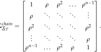
5.2.2. Chain approximation 306
The chain covariance matrix is as follows (nodes are connected like a first order Markov chain, 1 307
ton) 308
Σchain XT =
1 ρ ρ2 . . . ρn−1
ρ . .. ... ... ...
ρ2 . .. ... ... ρ2 ..
. . .. ... ... ρ
ρn−1 . . . ρ2 ρ 1
.
For this example, the KL divergence and the Jeffreys divergence can be computed in closed form as
D(X||Xchain) =D(X||Xstar) and
DJ(X, Xchain) =
ρ2
(1+ (n−1)ρ)(1−ρ)×
n(n−1)
2 −
n(1−ρn)
1−ρ +
1−(n+1)ρn+nρn+1 (1−ρ)2
respectively. Moreover, for large values ofnwe have the following approximation
DJ(X,Xchain)≈ n 2
ρ 1−ρ.
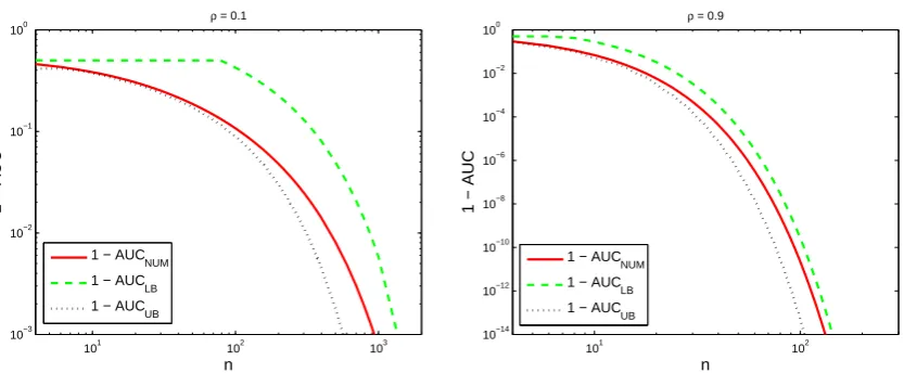
Figure7plots the 1−AUC v.s. the dimension of the graph,nfor different correlation coefficients, 309
ρ=0.1 andρ=0.9 as well as its upper and lower bounds. 310
In both figure6and figure7,(1−AUC)and its bounds rapidly goes to 0 which means that AUC 311
goes to one as we increase the number of nodes,n, in the graph. More precisely, bounds for 1−AUC 312
are decaying exponentially as the dimension of the graph,n, increases which is consistent with the 313
theory obtained for analytical bounds. Furthermore, we can conclude from these figures that a smaller 314
101 102 103 10−3
10−2 10−1 100
ρ = 0.1
1 − AUC
n
1 − AUC
NUM
1 − AUCLB 1 − AUC
UB
101 102
10−14 10−12 10−10 10−8 10−6 10−4 10−2 100
ρ = 0.9
1 − AUC
n
1 − AUC
NUM
1 − AUC
LB
1 − AUC
UB
Figure 7.1−AUC v.s. the dimension of the graph,nfor Chain approximation of the Toeplitz example withρ=0.1(left)andρ=0.9(right). In both figures, the numerically evaluated AUC is compared with its bounds.
are more like tree structure model. Moreover, comparing the AUC for the star network approximation 316
with the AUC for the chain network approximation we conclude that the star network is a much better 317
approximation than the chain network even though that both approximation networks have the same 318
KL divergences. We can also interpret this fact through the analytical bounds obtained in this paper. 319
The star network is a better approximation than the chain network since the decay rate of 1−AUC for 320
the star network is less than its decay rate for the chain network. 321
Remark:The star approximation in the above example has lower AUC than the chain approximation. 322
Practically, it means the correlation between nodes that are not connected in the approximated graphical 323
structure is more realistic in star network than the chain network. 324
5.3. Solar data 325
In this Example, covariance matrix is calculated based on datasets presented in [35]. Two datasets 326
which are obtained from the National Renewable Energy Laboratory (NREL) website [36]. The first 327
data set is the Oahu solar measurement grid which consists of 19 sensors (17 horizontal sensors and 328
two tilted sensors) and the second one is the NREL solar data for 6 sites near Denver, Colorado. These 329
two data sets are normalized using standard normalization method and the zenith angle normalization 330
method [35] and then the unbiased estimate of the correlation matrix is computed9. 331
5.3.1. The Oahu solar measurement grid dataset 332
From data obtained from 19 solar sensors at the island of Oahu, we computed the spatial 333
covariance matrix during the summer season at 12:00 PM averaged over a window of 5 minutes. 334
Then, the AUC and the KL divergence are computed for those tree structures that are generated using 335
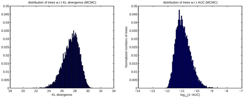
Markov Chain Monte-Carlo (MCMC) method. Figure8shows the distribution of those tree structures 336
generated using MCMC method versus the KL divergence(left)and v.s log10(1−AUC)(right)10. 337
Looking back at figure 4, for very small value of 1−AUC the relationship between the KL 338
divergence and the boundary of the possible feasible region for −log(1−AUC) is linear. This 339
means that if the upper bound is tight then the relationship between the KL divergence and the 340
9 See [35] for fields definition and other details about the normalization methods for the solar irradiation covariance matrix. 10 In this example, since the AUC for all generated tree structures is close to one, we plots the distribution of generated trees
5 10 15 20 0
0.005 0.01 0.015 0.02 0.025 0.03 0.035 0.04 0.045 0.05
KL divergence
Normalized numbers of trees
distribution of trees w.r.t KL divergence (MCMC)
−7.50 −7 −6.5 −6 −5.5 −5 −4.5 −4 −3.5 −3 −2.5 0.005
0.01 0.015 0.02 0.025 0.03 0.035 0.04
log10(1−AUC)
Normalized numbers of trees
distribution of trees w.r.t AUC (MCMC)
Figure 8. Left:distribution of the generated trees (Normalized histogram) using MCMC v.s. the KL divergence andRight:distribution of the generated trees (Normalized histogram) using MCMC v.s. log10(1−AUC)for the Oahu solar measurement grid dataset in summer season at 12:00 PM.
−log(1−AUC)is almost linear. In figure8, the maximum value of 1−AUC for this model is less than 341
10−3which justifies why two distributions in figure8are scaled/mirrored of each other. Moreover, 342
just by looking at the distribution of tree models in this example, it is obvious that most tree models 343
have similar performance. Only a small portion of the tree models have better performance than the 344
most trees, but the difference is not that significant. 345
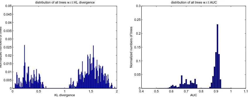
5.3.2. The Colorado dataset 346
From the solar data obtained from 6 sensors near Denver, Colorado, we computed the spatial 347
covariance matrix during the summer season at 12:00 PM averaged over a window of 5 minute. Then, 348
the AUC and the KL divergence are computed for all possible tree structures. Figure9shows the 349
distribution of all possible tree structures v.s the KL divergence(left)and v.s the AUC(right). 350
0 0.5 1 1.5 2
0 0.005 0.01 0.015 0.02 0.025 0.03 0.035 0.04 0.045 0.05
KL divergence
Normalized numbers of trees
distribution of all trees w.r.t KL divergence
0.4 0.5 0.6 0.7 0.8 0.9 1 1.1 0
0.05 0.1 0.15 0.2 0.25 0.3
AUC
Normalized numbers of trees
distribution of all trees w.r.t AUC
Figure 9. Left: distribution of all trees (Normalized histogram) v.s. the KL divergence andRight:
distribution of all trees (Normalized histogram) v.s. the AUC for the Colorado dataset in summer season at 12:00 PM.
In the Colorado dataset, there are two sensors that are very close to each other compared to the 351
distance between all other pairs of sensors. As a result, if the particular edge between these two sensors 352
particular edge is not in the tree structure. This explains why the distributions of all trees in this case 354
looks like a mixture of two distributions. This result also gives us valuable incite on how to answer the 355
following question, "How to construct informative approximation algorithms for model selection in 356
general." One catch as an example is that for the Colorado dataset, almost all trees that contain the 357
particular edge between the two aforementioned sensors are good approximations while the rest of 358
tree models’ performances are not desirable. 359
5.3.3. Two-dimensional sensor network 360
In this example, we create a 2-dimensional (2D) sensor network using Gaussian kernel [37] as follows
ΣX(i,j) =
e−
d(i,j)2
2σ2
whered(i,j)is the Euclidean distance between thei-th sensor and thej-th sensor in the 2D space. All 361
sensors are located randomly in 2D space11. We setσ=1 and generate a 2D sensor network with 20 362
sensors. For the 2D sensor network example, figure10shows the distribution of the generated tree 363
structures using MCMC method v.s KL divergence(left)and v.s log10(1−AUC)(right). Again we see 364
the mirroring effect in Fig.10as we have an almost linear relationship between the KL divergence and 365
−log(1−AUC). Note that, the covariance matrix generated has one dominant eigenvalue in most 366
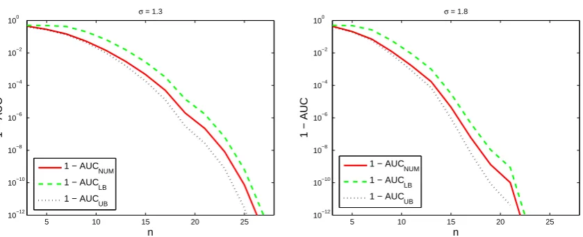
cases. Furthermore, figure11plots 1−AUC as well as its analytical upper bound and lower bound 367
v.s. the dimension of the graph,nforσ =1.3(left)andσ= 1.8(right). To generate this figure, we 368
randomly generated 1000 sensor networks and then plot the averaged AUC. As we can see in this 369
figure, the 1−AUC and its bounds decay exponentially which is consistent with the theoretical results 370
of this paper.
18 20 22 24 26 28 30 32 34 0
0.005 0.01 0.015 0.02 0.025 0.03 0.035 0.04 0.045 0.05
KL divergence
Normalized numbers of trees
distribution of trees w.r.t KL divergence (MCMC)
−140 −13 −12 −11 −10 −9 −8 −7 0.005
0.01 0.015 0.02 0.025 0.03 0.035 0.04 0.045 0.05
log10(1−AUC)
Normalized numbers of trees
distribution of trees w.r.t AUC (MCMC)
Figure 10. Left:distribution of the generated trees (Normalized histogram) using MCMC v.s. the KL divergence andRight:distribution of the generated trees (Normalized histogram) using MCMC v.s. log10(1−AUC)for the 2D sensor network example with 20 sensors andσ=1.
371
6. conclusion 372
In this paper, we formulate a detection problem and investigate the quality of model selection 373
problem. More specifically, we consider Gaussian distributions and discuss the covariance selection 374
quality of a given model. We present the correlation approximation matrix (CAM), and show its 375
relationship with information theory divergences such as the KL divergence, the reverse KL divergence 376
5 10 15 20 25 10−12
10−10 10−8 10−6 10−4 10−2 100
σ = 1.3
1 − AUC
n
1 − AUCNUM 1 − AUC
LB
1 − AUC
UB
5 10 15 20 25 10−12
10−10 10−8 10−6 10−4 10−2 100
σ = 1.8
1 − AUC
n
1 − AUC
NUM
1 − AUC
LB
1 − AUCUB
Figure 11.1−AUC and its bounds v.s. the dimension of the graph,nforσ=1.3(left)andσ=1.8
(right), averaged over 1000 runs of sensor networks generated randomly.
and the Jeffreys divergence as well as the ROC curve and the area under it, i.e. the AUC, as a 377
measure of accuracy in the detection problem framework. Moreover, this paper presents an analytical 378
expression for the AUC that can efficiently be evaluated numerically. Also, the AUC analytical lower 379
and upper bounds are provided in this paper. We show that the AUC and the lower bound for the 380
AUC depend on the eigenvalues of the CAM. Upper bounds for the AUC are obtain from finding 381
a parametric relationship between the AUC and the KL/reverse KL divergences. We pick the tree 382
structure as an example of an approximation model and use the Chow-Liu MST algorithm to compute 383
the maximum likelihood tree structure approximation. Then, the quality of the Chow-Liu MST tree 384
algorithm is investigated using the formulated detection problem. Through some examples, we show 385
that in general, the tree approximation is not a good model as the number of nodes in the graphical 386
model increases which is the case in high dimensional problems such as modeling the electrical 387
distribution grid using smart grid sensor measurements and distributed renewable energy sources. 388
The aforementioned result is also consistent with the analytical results provided in this paper that is 389
1−AUC decays exponentially as the dimension of graph increases. 390
The detection framework presented in this paper, can be generalized for non-Gaussian models. 391
Moreover, the AUC analytical bounds obtained in this paper can also be used in other applications 392
that are using AUC as a relevant criterion. One example is in medicine when the AUC is used for 393
diagnostic tests between positive instance and negative instance [38] where instead of changing the 394
coordinates we can look at the exponent of the AUC bounds. In ongoing work we are looking at more 395
accurate graphical approximations that involve non-tree graphs. These approximations use a variation 396
of the CAM which we call the symmetric CAM and simple linear transformations. 397
Acknowledgments:This paper was presented for the special case of tree approximation in part at 2016 Information
398
Theory and Application Workshop [25]. Authors would like to thank Prof. Peter Harremoës for his helpful
399
discussions on information divergences and assistance with Theorem3. This work was supported in part by NSF
400
grant ECCS-1310634, the Center for Science of Information (CSoI), an NSF Science and Technology Center, under
401
grant agreement CCF-0939370, and the University of Hawaii REIS project.
402
Conflicts of Interest:The authors declare no conflict of interest. The founding sponsors had no role in the design
403
of the study; in the collection, analyses, or interpretation of data; in the writing of the manuscript, and in the
404
decision to publish the results.
Appendix A Proof of Lemma1
406
The calculus based proof for the special case of continuous PDFs is as follow. We can apply the Leibniz integral rule [39] and compute the derivative of CDFsP0(l)andP1(l)as
fL0(l) =−dP0(l)
dl and
fL1(l) =−dP1(l)
dl since fL0(l)and fL1(l)are continuous functions.12 We have
D fL0(l)||fL1(l)
= Z +∞
−∞ log fL0(l)
fL1(l)
fL0(l)dl
(a)
= −
Z 1
0 log dP1 dP0dP0 (b)
= −
Z 1
0 logh 0(z)dz
where equality (a) is true since we can replace PDfs fL0(l)and fL1(l)using the derivative of their
407
CDFs. Equality (b) is just a change of variable,z=P0(l), in order to write the integral in terms of the 408
derivative of the ROC curve. Proof for the second part of this lemma is similar to the proof of the first 409
part.
410
Appendix B Proof of Theorem3
411
Looking back at properties of the ROC curve,h(z), wherez∈[0, 1], the ROC curve have to satisfy 412
the following conditions 413
• C1:R01h0(z)dz=1 414
• C2:h0(z)≥0 415
• C3:h0(z)is decreasing 416
whereh0(z)is the derivative of the ROC curve,h(z). Also for a given ROC curve,h(z), we can compute the AUC as
Pr(L∆>0) = Z 1
0 h (z)dz. Then, using integration by parts, we can show that
1−Pr(L∆>0) = Z 1
0 z h 0
(z)dz.
To compute the possible feasible region stated in the theorem3, we need to optimize both of 417
following KL divergences,D fL1(l)||fL0(l)
andD fL0(l)||fL1(l)
, with respect to the derivative of 418
the ROC curve given a fixed AUC, Pr(L∆>0), while conditions, C1, C2 and C3 hold. To solve this 419
optimization, we can use the method of Lagrange multiplier. 420
12 Bothf
L0(l)andfL1(l)are PDFs in generalized Chi-squared distributions class. This means that each of these PDFs are
First step:Here we minimizeD fL1(l)||fL0(l)
with respect to the derivative of the ROC curve given the constraints. Optimization problem is as follow
arg min h0(z)
−
Z 1
0 logh
0(z)dz (A1)
s. t. Z 1
0 z h
0(z)dz=1−Pr(L
∆>0)
C1, C2 & C3.
To solve this optimization problem, we first write the Lagrangian. We need two coefficientsaandb corresponding to conditions in optimization problem (A1). Then, we can write the Lagrange multiplier as a function of the derivative of the ROC curve,z,aandbas follow
L(h0(z),z,a,b) =−
Z 1
0 logh 0(z)dz
+a
Z 1
0 zh
0(z)dz−(1−Pr(L
∆>0))
+b
Z 1
0 h 0
(z)dz−1
.
Note that, the Lagrangian, L(h0(z),z,a,b)is a convex function of h0(z). Thus, we can compute its minimum by taking its derivative with respect toh0(z). Doing so, we get
∂L(h0(z),z,a,b) ∂h0(z) =
Z 1
0
az+b− 1
h0(z)
dz.
Set∂L(h0(z),z,a,b)
∂h0(z) =0 we get
h0(z) = 1 az+b
for allz∈[0, 1]. From C3, sinceh0(z)is decreasing, we can conclude thata>0. Moreover, from C1, at 421
optimum we haveR1
0 h0(z)dz=1 and thus, we can compute one of the coefficients asb= eaa−1.
422
Computing the AUC integral and the KL divergence using the ROC curve we get the following parametric boundary for the possible feasible region
Pr(L∆>0) = 1 1−e−a −
1
a (A2)
and
D=log(a) + a
ea−1−1−log(1−e
−a) (A3)
whereD=D fL1(l)||fL0(l)
. 423
Second step:Here we minimizeD fL0(l)||fL1(l)
. The Lagrange multiplier for this step is similar to the first step but it is more straight forward if we defineg(η) =h−1(η). Note that using integration by parts, we can show that AUC is
Pr(L∆>0) = Z 1
0 ηg 0(
η)dη.
Now, we can write the Lagrangian for the optimization problem with respect tog0(η). The Lagrangian is convex with respect tog0(η), thus taking the derivative and set it equal to zero as follow
we can compute the parametric boundary for the possible feasible region. The parametric boundary in this case is the same as solution in (A2) and (A3) withD=D fL0(l)||fL1(l)
. Thus, combining these two steps, for the optimal boundary we have
Dl∗=min{D fL1(l)||fL0(l)
,D fL0(l)||fL1(l)
}.
424
References 425
1. Dempster, A.P. Covariance selection. Biometrics1972,28, 157–175.
426
2. Chow, C.K.; Liu, C.N. Approximating discrete probability distributions with dependence trees. IEEE
427
Transactions on Information Theory1968, pp. 462–467.
428
3. Shuman, D.I.; Narang, S.K.; Frossard, P.; Ortega, A.; Vandergheynst, P. The emerging field of signal
429
processing on graphs: Extending high-dimensional data analysis to networks and other irregular domains.
430
Signal Processing Magazine, IEEE2013,30, 83–98.
431
4. Koller, D.; Friedman, N.Probabilistic graphical models: principles and techniques; MIT press, 2009.
432
5. Jordan, M.I.Learning in graphical models; Vol. 89, Springer Science & Business Media, 1998.
433
6. Lauritzen, S.L.Graphical models; Clarendon Press, 1996.
434
7. Kschischang, F.R.; Frey, B.J.; Loeliger, H.A. Factor graphs and the sum-product algorithm. Information
435
Theory, IEEE Transactions on2001,47, 498–519.
436
8. Loeliger, H.A.; Dauwels, J.; Hu, J.; Korl, S.; Ping, L.; Kschischang, F.R. The Factor Graph Approach to
437
Model-Based Signal Processing. Proceedings of the IEEE2007,95, 1295–1322.
438
9. Khajavi, N.T.; Kuh, A. First order Markov chain approximation of microgrid renewable generators
439
covariance matrix. Proc. of IEEE International Symposium on Information Theory, Istanbul, Turkey (ISIT’
440
13), 2013, pp. 1207–1211.
441
10. Meinshausen, N.; Buhlmann, P. Model selection through sparse maximum likelihood estimation.Annals of
442
Statistics2006, pp. 1436–1464.
443
11. Friedman, J.; Hastie, T.; Tibshirani, R. Sparse inverse covariance estimation with the graphical lasso.
444
Biostatistics2008,9, 432–441.
445
12. Kruskal, J.B. On the shortest spanning subtree of a graph and the traveling salesman problem. Proceedings
446
of the American Mathematical society1956,7, 48–50.
447
13. Prim, R.C. Shortest connection networks and some generalizations. Bell system technical journal1957,
448
36, 1389–1401.
449
14. Khajavi, N.T. Latent tree approximation in linear model. Acoustics, Speech and Signal Processing (ICASSP),
450
2017 IEEE International Conference on. IEEE, 2017, pp. 5940–5944.
451
15. Kadane, J.B.; Lazar, N.A. Methods and criteria for model selection. Journal of the American statistical
452
Association2004,99, 279–290.
453
16. MacKay, D.J.C.Information theory, inference, and learning algorithms; Vol. 7, Citeseer, 2003.
454
17. Jeffreys, H. An invariant form for the prior probability in estimation problems. Proceedings of the Royal
455
Society of London. Series A. Mathematical and Physical Sciences1946,186, 453–461.
456
18. Lewis-II, P.M. Approximating probability distributions to reduce storage requirements.Information and
457
control1959,2, 214–225.
458
19. Lehmann, E.L.; Romano, J.P.Testing statistical hypotheses; springer, 2006.
459
20. Neyman, J.; Pearson, E.S. On the use and interpretation of certain test criteria for purposes of statistical
460
inference.Biometrika1928,20.
461
21. Eguchi, S.; Copas, J. Interpreting Kullback–Leibler divergence with the Neyman–Pearson lemma. Journal
462
of Multivariate Analysis2006,97, 2034–2040.
463
22. Scharf, L.L.Statistical signal processing; Vol. 98, Addison-Wesley Reading, MA, 1991.
464
23. Shiryaev, A.N. Probability, volume 95 of Graduate texts in mathematics, 1996.
465
24. Hanley, J.A.; McNeil, B.J. The meaning and use of the area under a receiver operating characteristic (ROC)
466
curve.Radiology1982,143, 29–36.