Generalized Convolution Spectral Mixture for
Multi-task Gaussian Processes
Kai Chen
Shenzhen Institutes of Advanced Technology, Chinese Academy of Sciences Shenzhen College of Advanced Technology, University of Chinese Academy of Sciences
Institute for Computing and Information Sciences, Radboud University [email protected]
Twan van Laarhoven
Institute of Management, Science and Technology, Open University of the Netherlands Institute for Computing and Information Sciences, Radboud University
Perry Groot
Institute for Computing and Information Sciences, Radboud University [email protected]
Jinsong Chen
Shenzhen Institutes of Advanced Technology, Chinese Academy of Sciences [email protected]
Elena Marchiori
Institute for Computing and Information Sciences, Radboud University [email protected]
Abstract
1
Introduction
Gaussian Processes (GPs) are an elegant Bayesian approach to model an unknown function. They provide regression models where a posterior distribution over the unknown function is maintained as evidence is accumulated. This allows Gaussian processes to learn complex functions if a large amount of evidence is available and makes them robust against overfitting in the presence of little evidence [1, 2]. A GP can model a large class of phenomena through the choice of its kernel which characterizes one’s assumption on how the unknown function autocovaries. The choice of kernel, however, is a core aspect of the GP design, since the posterior distribution can significantly vary for different kernels. As a consequence, various kernels (e.g., Squared Exponential, Periodic, and Matérn) and kernel design methods have been proposed [2]. The extension of GPs to multiple sources of data is known as multi-task Gaussian processes (MTGPs). MTGPs model temporal or spatial relationships among infinitely many random variables, as scalar GPs, but also account for the statistical dependence across different sources of data (or tasks) [3, 4, 5, 6, 7, 8]. How to choose an appropriate kernel to jointly model the cross covariance between tasks and auto-covariance within each task is the core aspect of MTGPs design [9, 10, 11, 4, 12, 13].
Early approaches to MTGPs, like the Linear Model of Coregionalization (LMC [14, 3, 7] focu-sed on linear combinations of independent single-output GPs. More expressive methods like the multi-kernel method [11] and the convolved latent function framework [15, 16, 17, 18] consider convolution to construct cross-covariance functions, and assume that each task has its own kernel. The use of spectral mixture (SM) kernels has further boosted the development of MTGP methods. Specifically, the expressiveness power of MTGP methods with SM kernels has increased during the past years: first the SM-LMC kernel was proposed [19, 20], which just uses independent spectral mixtures and global linear weights; then the Cross-Spectral Mixture (CSM) kernel [21], a more flex-ible kernel which considers the power and phase correlation between multiple tasks. CSM cannot capture complicated cross correlations because it only considers phase dependencies between tasks. Therefore the Multi-Output Spectral Mixture kernel (MOSM) was proposed [22] which addresses this limitation. MOSM, however, considers task level correlations within each spectral mixture by using independent components. MOSM has three limitations: all tasks have the same number of components, components in different tasks should be aligned, and spectral mixture level depen-dency within each task is ignored. Recently the generalized convolution spectral mixture of coupling coregionalization (GCSM-CC) kernel [23] explicitly extended previous works to model nonlinear correlations between tasks and dependencies between spectral mixtures and introduced coupling coregionalization to learn task level correlations. This means GCSM-CC only addresses the last mentioned limitation of MOSM, but that, as a result of using coupling coregionalization [23], tasks in GCSM-CC share the same kernel, and hyper-parameters in coregionalization terms involving task correlations are global and linear.
In this paper we fully address structure modeling of task level correlations and spectral level depen-dencies in MTGP and propose the multi-task generalized convolution spectral mixture (MT-GCSM) kernel. In MT-GCSM, we consider a two-level type of dependency: at the task level and at the spectral mixture level using generalized convolution spectral mixture kernel [24]. Without the re-striction that all tasks should have the same number of components, both task level correlation and spectral mixture level dependency are fully convolved with time and phase delay. In the proposed kernel, each task has its own Generalized Convolution Spectral Mixture (GCSM) kernel [24] cha-racterized by the task structure. Notably, without increasing the hyper-parameter space, MT-GCSM can involve hundreds of convolution structures. When only a single task is available, MT-GCSM reduces to the GCSM which has been shown to be a generalization of the ordinary SM kernel.
Specifically, we address the following questions. (1) How to model spectral mixture level depen-dency within a task? (2) How to build generalized spectral mixtures between tasks for modeling task level correlation? (3) How to incorporate inner spectral mixture level dependency and cross task level correlation simultaneously? (4) What’s the relationship between MT-GCSM and other SM-based kernels?
synthe-tic and real-world datasets. A summary of the paper’s contributions, concluding remarks, and future work on this topic are given in the Section 7.
2
Backgroud
We start with some background information on GPs, multi-task GPs, and spectral mixture kernels.
2.1 Gaussian processes
A Gaussian process defines a distribution over functions, specified by its mean and covariance function [2]. The mean functionm(x)and covariance functionk(x, x⊤)can be written as
m(x) =E[f(x)] (1)
k(x, x⊤) =E[(f(x)−m(x))(f(x⊤)−m(x⊤))] (2)
where xis an arbitrary input variable in RP. The covariance function k mapping two random variables intoRP, is applied to construct a positive definite covariance matrix, here denoted byK. Givenm(x)andk(x), we can define a GP as
f(x)∼ GP(m(x), k(x, x⊤)) (3)
Without loss of generality we assume the mean of a GP to be zero. By placing a GP prior over functions through the choice of kernels and parameter initialization, and the training data, we can predict the unknown valuey¯∗and its varianceV[y∗](that is, its uncertainty) for a test pointx∗using the following key predictive equations for GP regression [2]:
¯
y∗=K⊤(x, x∗)(K(x,x⊤) +σn2I)−1y (4) V[y∗] =k(x∗, x∗)−K⊤(x, x∗)(K(x,x⊤) +σn2I)−1K(x, x∗) (5) wherexis an input vector andyis the observed value corresponding to inputx. Typically, GPs con-tain free parameters, called hyper-parameters, which can be optimized by minimizing the Negative Log Marginal Likelihood (NLML). The NLML is defined as follows:
NLML=−log p(y|x,Θ)
∝
model fit
z }| {
1 2y
⊤(K+σ2 nI)−
1y+
complexity penalty
z }| {
1
2log|K+σ
2 nI|
(6)
whereK=K(x,x⊤),Θare the hyper-parameters of the kernel function, andσ2
nis the noise level. The NLML above directly follows from the observation thaty∼N(0, K+σ2
nI).
In multi-task GP (MTGP), we have multiple sources of data which specify related tasks. The con-struction of the MTGP covariance function kMTGP models dependencies between pairs of points
from two tasks.
2.2 Spectral mixture kernel
Usually, the smoothness and generalization properties of GPs depend on the kernel function and its hyper-parametersΘ. Choosing an appropriate kernel function and its initial hyper-parameters based on prior knowledge from the data are the core steps of a GP. Various kernel functions have been proposed [2], such as Squared Exponential (SE), Periodic (PER), and general Matérn (MA). Recently new covariance kernels have been proposed in [19, 25], called Spectral Mixture (SM) kernels. A SM kernel, here denoted byKSM, is derived through modeling a spectral density (Fourier
transform of a kernel) with Gaussian mixtures. A desirable property of SM kernels is that they can be used to reconstruct other popular standard covariance kernels. According to Bochner’s Theorem [26], the properties of a stationary kernel entirely depend on its spectral density. With enough componentskSMcan approximate any stationary covariance kernel [25].
kSM(τ) =
Q
∑
q=1 wqcos
(
2πµqτ⊤
)∏P
p=1
exp
(
−2π2τ2Σ(qp)
)
whereQis the number of components,Pis the dimension of dataset,wq,µq =
[
µm q , ..., µ
(P) q
]
, and
Σq =diag
([
(σ2
q)m, ...,(σq2)(P)
])
are weight, mean, and variance of theq-th mixture component in frequency domain, respectively. The varianceσ2q can be thought of as an inverse length-scale,µq as a frequency, andwq as a contribution.
Bochner’s Theorem [26, 27] indicates a direction on how to construct a valid kernel from the fre-quency domain. This implies that this kind of kernels can also be transformed between time domain and frequency domain. Using the following definition, the spectral density of kernel functionk(τ)
can be given by its Fourier transform:
ˆ
k(s) =
∫ ∞
−∞
k(τ)e−2πιτ s˙ dτ (8)
Furthermore, the inverse Fourier transform of spectral densityˆk(s)is the original kernel function k(τ).
k(τ) =
∫ ∞
−∞
ˆ
k(s)e2πιτ s˙ ds (9)
We will use a hatˆk(s)to denote the spectral density of a covariance functionkin the frequency domain. From Bochner’s theorem [26, 27] k(τ)and ˆk(s)are Fourier duals of each other. For SM kernel [19], using Fourier transform of the spectral densitykˆSM(s) = [φSM(s) +φSM(−s)]/2
whereφSM(s) =N(s;µ,Σ)is a symmetrized scale-location mixture of Gaussians in the frequency
domain, we have
kSM(τ) =Fs−→1τ
[∑Q
q=1
wqˆkSM(s)
] (τ) = Q ∑ q=1
wqFs−→1τ[(φSM(s) +φSM(−s))/2
]
(τ)
(10)
3
Multi-task generalized convolution SM kernels
We now address the first three questions mentioned in Section 1.
3.1 Generalized convolution spectral mixture kernel within task
In [24] we used convolution to model spectral mixture level dependency with a quadratic number of convolution structures in a single task. The resulting GCSM kernel can be formalized as follow:
kGCSM(τ) =Fs−→1τ
[(∑Q
i=1
√
wiφGCSMi(s)
)
·
(∑Q
j=1
√
wjφGCSMj(s)
)
+
(∑Q
i=1
√
wiφGCSMi(−s)
)
·
(∑Q
j=1
√
wjφGCSMj(−s)
)] /2 = Q ∑ i=1 Q ∑ j=1 √w
iwj
√
4ΣiΣj
Σi+ Σj
1 2 exp ( −1
4(µi−µj)
⊤(Σ
i+ Σj)−1(µi−µj)
)
×exp
(
−π2(2τ−(θi−θj))
⊤ΣiΣj(2τ−(θi−θj))
Σi+ Σj
)
×cos
(
π
(
(2τ−(θi−θj))⊤(Σiµj+ Σjµi)
Σi+ Σj −
(ϕi−ϕj)
))
(11)
denotes the complex conjugate operator.
φGCSMi(s) =
1
√
(2π)P|Σi|exp
(
−(s−µi)⊤(s−µi)
2Σi
)
exp(−2πθisι˙−2πϕiι˙) (12)
whereθandϕare time delay and phase delay. Using GCSM we can model the dependency related to time and phase delay between spectral mixtures in a single task (see Figure 1). The single task GCSM can be seen as an inner full cross convolution spectral mixture in multi-task GCSM kernel.
Figure 1: GCSM and SM with the same number ofQbase spectral mixtures within a task. (a) the auto-convolution of base spectral mixtures in SM. (b) the cross and auto-convolution between base spectral mixtures in GCSM. Each circle represents a base spectral mixtures in GCSM. All circles have the same green color because they come from the same task.
3.2 Outer cross convolution spectral mixtures between tasks
Here we extend GCSM to a multi-task scenario. While in single task GP time and phase delay de-pendency exist within the task, in MTGP time and phase delay dependencies exist between different spectral mixtures from different tasks. Similar to GCSM in single task GPs, by considering distribu-tivity of convolution, we construct full cross convolution between, say, taskTmand taskTm′. Here
tasksTmandTm′ have different number of base spectral mixturesQ(m)andQ(m
′)
, respectively. Combining the inner full cross convolution of spectral mixtures within task (single task GCSM) and the outer full cross convolution spectral mixture between tasks, we can construct the so-called multi-task generalized convolution spectral mixture kernel (MT-GCSM), capable to model full de-pendency structure for MTGP at spectral mixture level. Here, time and phase delay dependencies are represented not only inside each task but also across tasks. The convolution relation is shown in Figure 2. The form of MT-GCSM between two tasksTmandTm′ is
kTm×Tm′
MT-GCSM(τ) =F−
1 s→τ
[(Q(m)
∑ i=1 √ wm i φ m
GCSMi(s)
)
·
(Q(m′)
∑
j=1
√
wm′
j φ m′
GCSMj(s)
)
+
(Q∑(m)
i=1
√
wm
i φmGCSMi(−s)
)
·
(Q∑(m′)
j=1
√
wm′ j φm
′
GCSMj(−s)
)]
/2
=
Q∑(m)
i=1 Q∑(m′)
j=1
√
wm i wm
′ j √ 4Σm i Σ m′ j Σm i + Σ
m′ j 1 2 ×exp ( −1
4(µ
m i −µm
′
j )⊤(Σmi + Σm
′
j )−1(µmi −µm
′
j )
)
×exp
(
−π2(2τ−(θ m i −θ
m′
j ))⊤Σmi Σm
′
j (2τ−(θ m i −θ
m′ j ))
Σmi + Σmj ′
)
×cos
(
π
((2τ−(θm i −θ
m′
j ))⊤(Σmi µm
′
j + Σm
′
j µmi )
Σm i + Σ
m′
j
−(ϕmi −ϕmj ′)
))
whereQ(m)andQ(m′)are the number of base spectral mixtures in tasksTmandTm′, respectively. In our setting, GCSM kernels in different tasks can have different number of spectral mixtures, depending on the task’s complexity. By analyzing the spectral density of a task in the frequency domain one can gain insight into its complexity. Note that existing SM-based kernels, for instance SM-LMC, MOSM and CSM, assume that all tasks should have the same number of spectral mixtures and that spectral mixtures should be aligned. Our kernel does not have such constraints.
Figure 2: Convolution relation in MT-GCSM. (a) mixture-wised dependencies in MOSM and Q(m)=Q(m′). (b) spectral mixture level dependent and task level coupled GCSM-CC with using the same GCSM kernel for all tasks. (c) MT-GCSM withQ(m)̸=Q(m′).
The proposed MT-GCSM kernel is illustrated in Figure 2. Each connection in MT-GCSM represents a convolution structure. While, for GCSM-CC and MT-GCSM, the dashed line in Figure 2 denotes the inner cross convolution structures. The solid lines in CGSM-CC and MT-GCSM are coupling coregionalization terms and outer cross convolution structures, respectively. Note that in GCSM-CC, tasksTmandTm′ share the same GCSM kernel, so the circles with the same green color.
Tasks in MT-GCSM have different number of components. When task1is equal to task2, there is no cross spectral mixture level convolution between tasks and the MT-GCSM reduces into GCSM. Furthermore, without considering spectral mixture dependencies, GCSM reduces into ordinary SM. All dashed lines in MT-GCSM can be seen as a set of inner component dependency. All solid lines in MT-GCSM can be seen as a set of cross tasks correlation. Both dashed lines and solid lines have the same convolution scale because both them based on convolution of base spectral mixtures.
In MT-GCSM, arbitrary MTGP kernelΩconstructed by MT-GCSM with arbitrary number of tasks fulfills the positive semi-definite condition (Ω≥0, the detailed proof is given in the appendix). The proof of positive semi-definite condition of MT-GCSM is different from that for GCSM because of the introduction of outer full cross convolution terms between tasks.
4
Relation to other kernels
Here we address the last question mentioned in Section 1. A lot of improvements and applications related to MTGPs have been achieved in previous works, like [3, 7, 11, 15, 20, 21, 22]. Since the introduction of SM kernels [25, 28], MTGPs with SM kernels [25, 28, 29, 30, 31, 32, 33] showed a strong learning ability and interpretation. Here we focus on MTGP methods based on such kernels [20, 21, 22]. The first MTGP using a SM kernel is based on the LMC framework [20] to construct a Gaussian process regression network (GPRN).
KSM-LMC=
Q
∑
q=1
Bq⊗KSMq (14)
TheBqinK
SM-LMCencodes cross weights to represent task correlations and involves a linear
contains cross phase spectrum and is also defined within the LMC framework as
KCSM=
Q
∑
q=1
BqkSG(τ; Θq) (15)
wherekSG(τ; Θq)is phasor notation of the spectral Gaussian kernel. The kernelskSG(τ; Θq)used in the CSM are, however, only phase dependent. The MOSM kernel [22] provides a principled framework to construct multivariate covariance functions with a better interpretation of cross relati-onships between tasks. MOSM has the form
kMOSMij (τ) =
Q
∑
q=1 αqijexp
(
−1
2(τ+θ
q ij)⊤Σ
q ij(τ+θ
q ij)
)
cos((τ+θqij)⊤µqij+ϕqij) (16)
whereαqij,θqij,Σqij,µqij, andϕqij are cross weight, cross time delay, cross covariance, cross mean, and cross phase delay between the i-th andj-th channels. SM-LMC and CSM are instances of MOSM. Even if MOSM improves upon existing methods in expressivity and interpretation, it still considers linear combinations of components and it ignores dependencies between spectral compo-nents.
A more recent SM based kernel for MTGP employs generalized convolution spectral mixture of coupling coregionalization (GCSM-CC) [23]. The GCSM-CC kernel is:
KGCSM-CC(τ) =
Q
∑
i=1 Q
∑
j=1
CiCj⊤⊗KGCSMi×GCSMj (17)
where CiCj⊤ term is the coupling coregionalization term and KGCSMi×GCSMj is the single task GCSM kernel. Although GCSM-CC considers both task level correlatons and spectral mixture level dependencies. GCSM-CC using coupling coregionalization, however, has the limitation that it shares the same kernel among tasks, which is a common drawback of MTGPs involving coregi-onalization [3]. Table 1 summarizes the characteristics of these kernels in terms of parameters and degrees of freedom.
Table 1: Comparisons between MT-GCSM and others. All LMC and coupling coregionalization terms use free form parameterization [3].
Kernel Parameters Degrees of freedom
SE-LMC {B, θf, θℓ} 2 + (M2+M)/2
Matérn-LMC {B, θf, θℓ} 2 + (M2+M)/2
SM-LMC {Bq,µ
q,Σq}Qq=1 Q(2P+ 1 + (M2+M)/2) CSM {σq, µq,{wq
r,ϕ q r, ϕ1rq
∆
=0}M r=1}
Q
q=1 2Q+M(2Q−1)
MOSM {{wq
m,µqm,Σqm,θ q
m, ϕqm}Mm=1} Q
q=1 QM(3P+ 2) GCSM-CC {Bq, wq,µq,Σq,θq,ϕq}
Q
q=1 Q(4P+ 1 + (M
2+M)/2)
MT-GCSM {{wmq ,µmq ,Σmq ,θ m q ,ϕ
m q }
Q(m) q=1 }
M m=1
M
∑
m=1
Q(m)(4P+ 1)
5
Interpretation of the dependencies modeled in MT-GCSM
MT-GCSM combines the advantages of MOSM and GCSM-CC without the above mentioned con-straints, and is therefore more flexible and expressive. In this section we illustrate the dependencies modeled in MT-GCSM.
(a) (b) (c) (d)
(e) (f) (g) (h)
Figure 3: Cross covariance and corresponding spectral densities between tasks inkTm×Tm′
MT-GCSM(τ). The
first row are zero time and phase delay, non-zero time delay and zero phase delay, zero time delay and non-zero phase delay, non-zero time and phase delay outer cross convolution structures of task T1(Q(1)= 2) and taskT2(Q(2)= 2) in MT-GCSM. The orange bolder solid lines are sum of outer cross convolution structures in MT-GCSM. The second row are corresponding spectral densities of the first row. For spectral densities of outer cross convolution structures, real part in solid line and imaginary part in dashed line.
give the four outer full cross convolution structures (see Equation (13)) because the four inner full convolution structures are given by single task GCSM (see Equation (11) [24]). The first row in Figure 3 show four full cross convolution structures (solid line with different color) in MT-GCSM and its sum respectively. From the last row in Figure 4, We can see the corresponding cross spectral densities in the frequency domain. Analyzing Equation 13 demonstrates that closer frequencies (µm
i ,µm
′
j ), scales (Σmi ,Σm
′
j ), and weights (wmi , wm
′
j ) between tasksTmandTm′ in MT-GCSM, induce stronger cross dependencies.
6
Experiments
In general, SM based kernels are sensitive to the initialization of its hyper-parameters, which can lead to a local optimal solution for NLML (see Equation 6). MT-GCSM kernel has the same initialization problem. In MT-GCSM, the degrees of freedom and parameter space areMtimes as large compared to using GCSM with a single task. Hyper-parameters initialization has a direct impact on the ability to discover and extrapolate patterns, especially in the presence of complex multiple tasks. Therefore we apply an initialization strategy which uses the empirical spectral density, which has been shown to be effective in other contexts [25]. The empirical spectral density is, however, often noisy, so its direct use is not possible. Past research suggests that sharp peaks of the empirical spectral density are near the true frequencies [25, 34]. We make use of this observation, and apply a Bayesian Gaussian mixture modelp(θ|s) =∑Qi=1w˜iN( ˜µi,Σ˜i)on the empirical spectral densitysin order to get the Qcluster centers of the Gaussian spectral density. We use the Expectation Maximization algorithm [35] to estimate the parametersw˜i,µ˜i, andΣ˜i. The results are used as initial values ofwi, µi, andΣiin each task, respectively. Then the time and phase delay parameters{θi,ϕi}are randomly initialized for each task in MT-GCSM. We use this technique in all our experiments on artificial and real world data.
task for all experiments. First we show the ability of MT-GCSM to model a mixed signal sampled from a Gaussian distribution specified byGP(0, KSM(Q= 3)), its integral and derivative, and its
time delayed signal simultaneously. Then we use MT-GCSM for prediction tasks on a real-world problem with two sensor array datasets: humidity monitoring related to climate change, Nitrogen dioxide (NO2) concentration related to air pollution. We implemented our models in Tensorflow [36] and GPflow [37] to improve scalability and to facilitate gradient computation. In all experiments we use the mean absolute errorMAE =∑ni=1|yi−y˜i|/nas performance metric.
6.1 Learning Signal, integral, derivative and time delayed signal simultaneously
We design an artificial experiment in order to validate the interpolation, extrapolation, signal reco-very, and block miss filling ability of MT-GCSM and compare its structure learning performance with that of other MTGP methods. We generate four nonlinear correlated tasks: a mixed signal, its integral, its derivative, and its time delay, respectively. Specifically, we sample a Gaussian signal f(x)∼ GP(0, KSM(Q= 3))with length 300 in the interval [-10, 10], numerically compute its first
integral and derivative, and delay the signal withf(x) =f(x+t),(t= 2).
From the signalf(x) we randomly choose half of the data as training data, and the rest as test data. The integration signal points in the interval [-10, 0] are used for training (in cyan), while the remaining signal points in the interval [0, 10] are used for testing (in green). For the third task, the derivative of the signal, data in the interval [0, 10] is used for training and the rest is used for testing. In the fourth task, signal points in the intervals [7, 10] and [-8, -3] are used for training and the rest of the points in the middle interval [-3, 7] are used for testing.
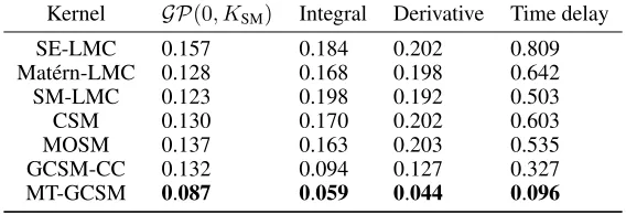
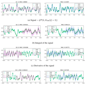
The performance of MT-GCSM on the generated signal is shown in Figure 4a. As shown in Table 2, all considered GP methods have comparable performance: they learn the covariance between tasks and are able to interpolate missing values well. The second task, i.e., the integral of the signal, is shown in Figure 4b. In this case its inherent patterns are more difficult to recognize and extrapolate. Here MT-GCSM and GCSM-CC perform better than other methods, but MT-GCSM achieves lowest MAE as well as smallest confidence interval. Both MT-GCSM and GCSM-CC excel also on the last two tasks. For instance, the derivative signal (Figure 4c) and the time delay signal (Figure 4d): here MT-GCSM and GCSM-CC show stronger pattern learning and extrapolation capability, with MT-GCSM having the best performance. Predictions obtained using SE-LMC and Matérn-LMC kernels are of low quality, especially for the long range extrapolation tasks (integral, derivative, and time delay signals): it is very hard for them to find valid patterns in the data, like the change of trend over time. Overall, results indicate the capability of MT-GCSM to capture integration and differentiation patterns of the generated signal simultaneously. Note that here SM-LMC, CSM, MOSM, GCSM-CC have the sameQ = 10with 10, 10, 10, and 100 components, respectively, but MT-GCSM has a different number of base spectral mixtures for each task (Q(1)= 4, Q(2) = 5, Q(3) = 6,Q(4) = 5). In total, we have ∑4i=1∑4j=1Q(i)Q(j) = 400convolution structures (102 inner convolution structures and 298 outer convolution structures) in MT-GCSM, which can capture far more structures in the data without the need of using extra hyper-parameters. As result of applying full cross convolution and considering complexity diversity of tasks, MT-GCSM using less number of components can learn patterns and dependencies better than the other kernels. Table 2 shows that only MT-GCSM gives a MAE smaller than 0.1 for all tasks, indicating the advantage of MT-GCSM compared to other kernels.
Table 2: Performance comparisons between MT-GCSM and others kernels on artificial dataset. The MT-GCSM kernel consistently presents the lowest MAE.
Kernel GP(0, KSM) Integral Derivative Time delay
SE-LMC 0.157 0.184 0.202 0.809
Matérn-LMC 0.128 0.168 0.198 0.642
SM-LMC 0.123 0.198 0.192 0.503
CSM 0.130 0.170 0.202 0.603
MOSM 0.137 0.163 0.203 0.535
GCSM-CC 0.132 0.094 0.127 0.327
(a) Signal∼ GP(0, KSM(Q= 3))
(b) Integral of the signal
(c) Derivative of the signal
(d) Task level time delayed signal
Figure 4: Performance of MT-GCSM (in dashed magenta line) and GCSM-CC (in dashed blue line) on artificial dataset. The shaded area shows the predicted variance. In this case only MT-GCSM can correctly learning the structure of four tasks simultaneously.
6.2 Humidity long range extrapolation
Sensor networks monitoring climate change in Stockholm city1provide historical analysis and
infor-mation about the future evolution of the regional environment. The recording allows us a possibility to extrapolate long range meteorological parameters such as humidity, which could guide environ-mental policy making. On the other hand, meteorological parameters are one of the main factors affecting local air pollution because they determine how air pollutant spreads. The humidity mo-nitoring recordings are recorded from a number of stations (Torkel Knutssonsgatan, Marsta, Norr Malma, Högdalen) in Stockholm and outside. For instance: Torkel Knutssonsgatan’s measurement at urban background, Marsta’s measurement and Högdalen’s measurement at a high-altitude tower, North Malma’s measurement at the regional background. Stockholm as a seaside city, the change of humidity in the city not only depends on weather conditions but also depends on its geographical location and surroundings. For example, stations located in the same area definitely have the same weather condition but will have totally different humidity values, because stations located nearby river or seaside will have higher humidity values. These factors are time and phase dependent with different scales.
1
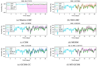
In this case, we use humidity time series from 05 November 2017 to 25 November 2017, in 1 hour intervals. Considering the advantage of structure learning and complexity diversity in MT-GCSM, here we set less number of componentsQ(1) = 5,Q(2) = 6, Q(3) = 7, andQ(4) = 5for task 1, task 2, task 3, and task 4, respectively. Here, randomly chosen half of humidity data in Torkel Knutssonsgatan (task 1), the first half of humidity data in Marsta (task 2), the last half of humidity data in Norr Malma (task 3), the first quarter and last quarter of humidity data in Högdalen (task 4) are used for training, the last half of humidity data in Marsta and the middle part of humidity data in Högdalen are used for testing. We aim to extrapolate the long range missing values of humidity data in Marsta and middle block missing values of humidity data in Högdalen. From Figure 5, we can see that there are no stable background environment values in the humidity recording. Interestingly, over time high peaks in humidity are more stable than low peaks. From Figure 5, in addition to time and phase dependent patterns within tasks (local patterns depending on surroundings) and time and phase dependent patterns cross tasks (global patterns depending on seasonal or yearly factors), we observe that the low peaks in humidity appear irregularly. The change in humidity is complicated and caused by the nonlinear interaction of local and global patterns. Therefore data from multiple stations should help when used to model long range extrapolation trends. Results indicate that all SM based kernels can extrapolate the humidity well, with MT-GCSM consistently achieving better performance in terms of MAE and predicted confidence interval (see Figure 5 and Table 3).
(a) Matérn-LMC (b) SM-LMC
(c) CSM (d) MOSM
(e) GCSM-CC (f) MT-GCSM
Figure 5: Performance comparison between MT-GCSM and other kernels on long range humidity extrapolation: (a) Matérn-LMC (in pink dashed line), (b) SM-LMC (in red dashed line), (c) CSM (in purple dashed line), (d) MOSM (in plum dashed line), (e) GCSM-CC (in blue dashed line), (f) MT-GCSM (in dashed magenta line) configuredQ={5,6,7,5}for tasks. The shaded area shows the predicted variance.
6.3 Nitrogen dioxide concentration long range extrapolation
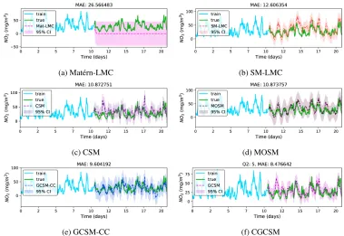
Sveavägen’s, and Norrlandsgatan’s measurement at a street. All recordings cover 24 hours at 1 hour interval and missing values are filtered. Each station corresponds to a task: Essingeleden as task 1, Hornsgatan as task 2, Sveavägen as task 3, and Norrlandsgatan as task 4. NO2 evolution has time and phase related patterns. Different stations have different local patterns which depend on the station’s surroundings. Still, these tasks have shared global trends because of the global seasonal change and periodic characteristics of human and industry activities. The evolution of NO2 concen-tration in each task is a result of nonlinear interaction of time and phase dependent local and global patterns.
In this case, we consider the recording time for NO2concentration from 25 July, 2017 to 15 August, 2017. From Figure 6, in addition to time and phase dependent global trends (global patterns depen-ding on seasonal or yearly factors) cross tasks and local patterns (local patterns dependepen-ding on local human activities and surrounding) within task, we observe that the high peaks in NO2appear non-periodically. Here we randomly choose half of NO2data in Essingeleden, the first half of NO2data in Hornsgatan, the last half of NO2data in Sveavägen, and the first quarter and last quarter of NO2 data in Norrlandsgatan for training. The last half of NO2data in Hornsgatan and the middle part of NO2 data in Norrlandsgatan are used for testing. We aim to extrapolate the long range missing values of NO2data in Hornsgatan and middle block missing values of NO2 data in Norrlandsga-tan. In this case, we aiming to give learning superiority of MT-GCSM even with less number of components for each task. Taking complexity diversity of tasks in account, we useQ={4,5,5,4}
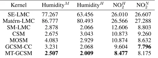
for MT-GCSM andQ = 10for the other kernels. Results indicate that all SM based kernels can extrapolate the future NO2concentration well, with MT-GCSM achieving the best performance (see Figure 6 and Table 3) in task 3 and GCSM-CC achieving the best performance in task 4. In this experiment, GCSM based kernels perform better than other kernels, which means there are indeed dependent structure in the NO2 concentration data. Actually predictions using the SE-LMC and Matérn-LMC cannot discover any valid patterns (see Figure 6a).
(a) Matérn-LMC (b) SM-LMC
(c) CSM (d) MOSM
(e) GCSM-CC (f) CGCSM
Table 3: Performance comparison between MT-GCSM and other kernels on real world datasets. The superscript M and H in humidity are Marsta station and Högdalen station, respectively. The superscript H and N in NO2are Hornsgatan station and Norrlandsgatan station, respectively
Kernel HumidityM HumidityH NOH2 NON2
SE-LMC 77.267 63.456 26.010 26.607
Matérn-LMC 86.777 80.493 26.566 27.288
SM-LMC 2.878 2.066 12.606 8.803
CSM 2.675 3.043 10.873 9.260
MOSM 4.083 2.929 10.874 8.632
GCSM-CC 3.231 2.068 9.604 7.796
MT-GCSM 2.507 2.009 8.477 8.175
7
Discussion
We proposed the multi-task generalized convolution spectral mixture (MT-GCSM) kernel to model dependent structures in tasks and across tasks. MT-GCSM is able to extrapolate multiple complex tasks simultaneously by using inner and cross convolution of time and phase dependent spectral mixtures. Experiments on artificial and real world datasets have shown the superiority that the MT-GCSM with less number of components for each task, is capable to exploit task level correlation and spectral mixture level dependency at the spectral mixture scale in the frequency domain. When used in multitask GPs, MT-GCSM can recognize and model complex structure in data, discover nonlinear correlation between tasks, and can make long-term extrapolations. Notably, MT-GCSM allows tasks to have a different number of components, which is more natural, as each task cannot be guaranteed to have the same number of patterns.
The proposed MT-GCSM kernel is an extension of previous work to discover spectral mixture level dependency within a task as well as task level nonlinear correlation between tasks. A limitation of the proposed kernel, shared by MTGPs which use multiple kernels, is the resulting relative inefficient inference. Sparse approximation and Bayesian optimization can be adopted as an improvement in efficient inference and hyper-parameters initialization [32, 38, 39, 40], which should improve the scalability of MT-GCSM. Currently efficient inference approximation methods like FITC and PITC [15, 16, 41, 42, 43], are not very effective for MTGPs using a multi-kernel framework. Future research will focus on sparse representations or efficient inference of the MT-GCSM.
Acknowledgement
This work was partly supported by China Scholarship Council (CSC).
References
[1] C. E. Rasmussen and H. Nickisch, “Gaussian processes for machine learning (gpml) toolbox,” Journal of Machine Learning Research, vol. 11, no. Nov, pp. 3011–3015, 2010.
[2] C. E. Rasmussen, Gaussian processes for machine learning, ser. Adaptive computation and machine learning, C. K. I. Williams, Ed. Cambridge, Massachusetts: The MIT Press, 2006.
[3] E. V. Bonilla, K. M. Chai, and C. Williams, “Multi-task Gaussian process prediction,” in Ad-vances in neural information processing systems, 2008, pp. 153–160.
[4] Z. Xu and K. Kersting, “Multi-task learning with task relations,” inProc. IEEE 11th Int. Conf. Data Mining, Dec. 2011, pp. 884–893.
[5] H. Kang and S. Choi, “Bayesian multi-task learning for common spatial patterns,” inProc. Int. Workshop Pattern Recognition in NeuroImaging, May 2011, pp. 61–64.
[7] R. Dürichen, M. A. Pimentel, L. Clifton, A. Schweikard, and D. A. Clifton, “Multitask Gaus-sian processes for multivariate physiological time-series analysis,”IEEE Transactions on Bio-medical Engineering, vol. 62, no. 1, pp. 314–322, 2015.
[8] W. Ruan, A. B. Milstein, W. Blackwell, and E. L. Miller, “Multiple output Gaussian process regression algorithm for multi-frequency scattered data interpolation,” inProc. IEEE Int. Geo-science and Remote Sensing Symp. (IGARSS), Jul. 2017, pp. 3992–3995.
[9] T. V. Nguyen and E. V. Bonilla, “Collaborative multi-output Gaussian processes,” in Proceedings of the Thirtieth Conference on Uncertainty in Artificial Intelligence, UAI 2014, Quebec City, Quebec, Canada, July 23-27, 2014, N. L. Zhang and J. Tian, Eds. AUAI Press, 2014, pp. 643–652. [Online]. Available: https://dslpitt.org/uai/displayArticleDetails. jsp?mmnu=1&smnu=2&article_id=2500&proceeding_id=30
[10] H. Wackernagel, “Multivariate geostatistics, 387 pp,” 2003.
[11] A. Melkumyan and F. Ramos, “Multi-kernel Gaussian processes,” in IJCAI Proceedings-International Joint Conference on Artificial Intelligence, vol. 22, no. 1, 2011, p. 1408.
[12] I. Bilionis and N. Zabaras, “Multi-output local Gaussian process regression: applications to uncertainty quantification,” Journal of Computational Physics, vol. 231, no. 17, pp. 5718– 5746, 2012.
[13] B. Zhang, B. A. Konomi, H. Sang, G. Karagiannis, and G. Lin, “Full scale multi-output Gaus-sian process emulator with nonseparable auto-covariance functions,”Journal of Computational Physics, vol. 300, pp. 623–642, 2015.
[14] P. Goovaerts, “Geostatistics for natural resources evaluation. oxford univ. press, new york.” Geostatistics for natural resources evaluation. Oxford Univ. Press, New York., 1997.
[15] M. Alvarez and N. D. Lawrence, “Sparse convolved Gaussian processes for multi-output re-gression,” inAdvances in neural information processing systems, 2009, pp. 57–64.
[16] M. A. Álvarez and N. D. Lawrence, “Computationally efficient convolved multiple output Gaussian processes,”Journal of Machine Learning Research, vol. 12, no. May, pp. 1459–1500, 2011.
[17] S. Gómez-González, M. A. Álvarez, H. F. García, J. I. Ríos, and A. A. Orozco, “Discriminative training for convolved multiple-output Gaussian processes,” in Iberoamerican Congress on Pattern Recognition. Springer, 2015, pp. 595–602.
[18] C. Guarnizo and M. A. Álvarez, “Fast kernel approximations for latent force models and con-volved multiple-output Gaussian processes,”arXiv preprint arXiv:1805.07460, 2018.
[19] A. G. Wilson, “Covariance kernels for fast automatic pattern discovery and extrapolation with Gaussian processes,”University of Cambridge, 2014.
[20] A. G. Wilson, D. A. Knowles, and Z. Ghahramani, “Gaussian process regression networks,” arXiv preprint arXiv:1110.4411, 2011.
[21] K. R. Ulrich, D. E. Carlson, K. Dzirasa, and L. Carin, “GP kernels for cross-spectrum analysis,” inAdvances in neural information processing systems, 2015, pp. 1999–2007.
[22] G. Parra and F. Tobar, “Spectral mixture kernels for multi-output Gaussian processes,” in Ad-vances in Neural Information Processing Systems, 2017, pp. 6684–6693.
[23] K. Chen, P. Groot, J. Chen, and E. Marchiori, “Generalized Spectral Mixture Kernels for Multi-Task Gaussian Processes,”ArXiv e-prints, Aug. 2018.
[24] ——, “Spectral Mixture Kernels with Time and Phase Delay Dependencies,”ArXiv e-prints, Aug. 2018.
[25] A. Wilson and R. Adams, “Gaussian process kernels for pattern discovery and extrapolation,” inProceedings of the 30th International Conference on Machine Learning (ICML-13), 2013, pp. 1067–1075.
[26] S. Bochner,Lectures on Fourier Integrals.(AM-42). Princeton University Press, 2016, vol. 42.
[27] M. Stein, “Interpolation of spatial data: some theory for kriging. 1999.”
[29] D. Duvenaud, J. R. Lloyd, R. Grosse, J. B. Tenenbaum, and Z. Ghahramani, “Structure discovery in nonparametric regression through compositional kernel search,” arXiv preprint arXiv:1302.4922, 2013.
[30] S. Flaxman, A. Wilson, D. Neill, H. Nickisch, and A. Smola, “Fast kronecker inference in Gaussian processes with non-gaussian likelihoods,” in International Conference on Machine Learning, 2015, pp. 607–616.
[31] J. B. Oliva, A. Dubey, A. G. Wilson, B. Póczos, J. Schneider, and E. P. Xing, “Bayesian nonparametric kernel-learning,” inArtificial Intelligence and Statistics, 2016, pp. 1078–1086.
[32] P. A. Jang, A. Loeb, M. Davidow, and A. G. Wilson, “Scalable Levy process priors for spectral kernel learning,” inAdvances in Neural Information Processing Systems, 2017, pp. 3943–3952.
[33] S. Remes, M. Heinonen, and S. Kaski, “A mutually-dependent hadamard kernel for modelling latent variable couplings,” inAsian Conference on Machine Learning, 2017, pp. 455–470.
[34] W. Herlands, A. Wilson, H. Nickisch, S. Flaxman, D. Neill, W. Van Panhuis, and E. Xing, “Scalable gaussian processes for characterizing multidimensional change surfaces,” inArtificial
Intelligence and Statistics, 2016, pp. 1013–1021.
[35] T. K. Moon, “The expectation-maximization algorithm,”IEEE Signal Processing Magazine, vol. 13, no. 6, pp. 47–60, 1997.
[36] M. Abadi, P. Barham, J. Chen, Z. Chen, A. Davis, J. Dean, M. Devin, S. Ghemawat, G. Irving, M. Isardet al., “Tensorflow: A system for large-scale machine learning. arxiv preprint,”arXiv preprint arXiv:1605.08695, 2016.
[37] A. G. d. G. Matthews, M. van der Wilk, T. Nickson, K. Fujii, A. Boukouvalas, P. León-Villagrá, Z. Ghahramani, and J. Hensman, “GPflow: A Gaussian process library using tensorflow,” Jour-nal of Machine Learning Research, vol. 18, no. 40, pp. 1–6, 2017.
[38] K. Swersky, J. Snoek, and R. P. Adams, “Multi-task Bayesian optimization,” inAdvances in neural information processing systems, 2013, pp. 2004–2012.
[39] R. Martinez-Cantin, “Bayesopt: A Bayesian optimization library for nonlinear optimization, experimental design and bandits,”The Journal of Machine Learning Research, vol. 15, no. 1, pp. 3735–3739, 2014.
[40] N. Knudde, J. van der Herten, T. Dhaene, and I. Couckuyt, “GPflowopt: A Bayesian optimiza-tion library using tensorflow,”arXiv preprint arXiv:1711.03845, 2017.
[41] Y. Wang and R. Khardon, “Sparse Gaussian processes for multi-task learning,” inJoint Euro-pean Conference on Machine Learning and Knowledge Discovery in Databases. Springer, 2012, pp. 711–727.
[42] J. Quiñonero-Candela and C. E. Rasmussen, “A unifying view of sparse approximate Gaussian process regression,”Journal of Machine Learning Research, vol. 6, no. Dec, pp. 1939–1959, 2005.
Supplementary
A Positive semi-definite condition of MT-GCSM
The proof of positive semi-definite condition of MT-GCSM is different from single task GCSM because of the introduction of outer cross convolution terms between tasks. In MT-GCSM, given samples {x(1)1 , x(1)2 , ..., x(1)n } ∈ task(1) and{x
(2) 1 , x
(2) 2 , ..., x
(2)
m} ∈ task(2), if there are arbitrary numbers{a(1)1 , a(1)2 , ..., a(1)n }and{a
(2) 1 , a
(2) 2 , ..., a
(2)
m}, we have a quadratic form
KMT-GCSM(x(1), x(2)) =Ω
= (A, A′)
(
Ω11 Ω12
Ω21 Ω22
)(
A⊤ A′⊤
) (18)
where
A={a(1)1 , a(1)2 , ..., a(1)n }
A′ ={a(2)1 , a(2)2 , ..., a(2)m}
Ω11={K1,1(x (1) i , x
(1) j )}
n i,j=1
Ω22={K2,2(xl(2), xt(2))}ml,t=1
Ω12={K1,2(x (1) i , x
(2) t )}
n;m i=1;t=1
Ω21={K2,1(x (2) l , x
(1) j )}
m;n l=1;j=1
(19)
According to Equation 11, we have the integral form ofKGCSMin each task.
KGCSM1,1 (x(1), x(1)′) =
∫ +∞ −∞ Q(1) ∑ q1=1 Q(1) ∑ q2=1
gq1(1)(x(1)−u)g(1)q2 (x(1)′−u)du
KGCSM2,2 (x(2), x(2)′) =
∫ +∞ −∞ Q(2) ∑ q1=1 Q(2) ∑ q2=1
gq1(2)(x(2)−u)g(2)q2 (x(2)′−u)du
KGCSM1,2 (x(1), x(2)) =
∫ +∞ −∞ Q(1) ∑ q1=1 Q(2) ∑ q2=1
gq1(1)(x(1)−u)g(2)q2 (x(2)−u)du
KGCSM2,1 (x(2), x(1)) =
∫ +∞ −∞ Q(2) ∑ q1=1 Q(1) ∑ q2=1
gq1(2)(x(1)−u)g(1)q2 (x(2)−u)du
(20)
Then
Ω=AΩ11A⊤+A′Ω21A⊤+AΩ12A′⊤+A′Ω22A′⊤
=
∫ +∞
−∞
(∑n
i=1 Q(1)
∑
q1=1
a(1)i gq(1)1 (x (1) i −u) +
m
∑
l=1 Q(2)
∑
q2=1
a(2)l gq(2)2 (x (1) l −u)
)2 ≥0
(21)


![Table 1: Comparisons between MT-GCSM and others. All LMC and coupling coregionalizationterms use free form parameterization [3].](https://thumb-us.123doks.com/thumbv2/123dok_us/1028488.1603011/7.612.129.483.463.590/table-comparisons-gcsm-lmc-coupling-coregionalizationterms-free-parameterization.webp)