Prediction and control of the motions of marine structures

(1)

PREDICTION AND CONTROL OF THE MOTIONS OF

MARINE STRUCTURES

by

Balwinder Singh Samra

Thesis submitted for the degree of DOCTOR OF PHILOSOPHY

in the

Faculty of Engineering University College London

University of London July 1993

(2)

ProQuest Number: 10105721

INFORMATION TO ALL USERS

The quality of this reproduction is dependent upon the quality of the copy submitted.

In the unlikely event that the author did not send a complete manuscript and there are missing pages, these will be noted. Also, if material had to be removed,

a note will indicate the deletion.

uest.

ProQuest 10105721

Published by ProQuest LLC(2016). Copyright of the Dissertation is held by the Author.

This work is protected against unauthorized copying under Title 17, United States Code. Microform Edition © ProQuest LLC.

ProQuest LLC

789 East Eisenhower Parkway P.O. Box 1346

(3)

ABSTRACT

This thesis reports the application of real time prediction and control techniques to mitigate problems caused by the motions of compliant marine structures.

Simulations and real ship motion data are used to assess an adaptive predictor. Practical points such as the appropriate choice and modification of forgetting factors, selection of sampling interval, effectiveness of concatenation and recursion of the Diophantine equation to generate multistep predictions are highlighted. Such aspects are vital to applications but hard to derive from theory. Ship motion data is used to assess the predictor as an operator guide. The predictions are shown to be useful in reducing waveoffs and crashes in VTOL operations at sea.

A predictor/controller system for crane barge loading operations in rough seas with constraints on control is developed using optimal control and a novel arrangement of model based predictive control (MBPC) techniques. The importance of constraints is emphasized and the MBPC techniques are shown to offer an efficient method of dealing with constraints.

Frequency domain techniques are used to design a motion suppression controller for a pneumatic semisubmersible - the exorbitant demanded control inputs shows the engineering impracticality of such a scheme.

(4)

To Miguel and Nieves

ACKNOWLEDGEMENTS

I would like to thank my supervisor for much of my period at UCL, Rick Jefferys for his guidance, constant help, enthusiasm and good humour. Dave Broome for his help in getting this thesis completed and his support during my time in his Control Laboratory at UCL.

Many thanks to my colleagues and friends for the many educative and enjoyable discussions. The Science and Engineering Research Council and industrial sponsors for generous financial support of this project. Adrian Lloyd of the Royal Navy who kindly supplied the ship motion data and Steve Bishop for some informative illustrations.

(5)

List of Tables

Chapter 4

Table 4.1 Table 4.2 Table 4.3

F and Akaike Tests

Sensitivity of F and AIC Barge Prediction

129 129 130

Chapter 5

Table Table Table 5.3

F and AIC for Ship Roll Data

Roll Prediction with Auxiliary Inputs and Nonlinear Regressors

Predictor Performance as an Operator Guide

185 185 186

Chapter 6

Table Table Table Table

Chapter 7

Table 7.1 Table 7.2

Control Input Cost - PSS Controller Predicted Peak and Time

Controller Profiles

Clipped Forms of Constrained Control

Some Generic Catastrophes Pole Position Variation With Mooring Arm Length

259 259 260 260

310

(10)

List of Figures

Chapter 2

Figure 2.1 Feedback Realization of Observer

Figure 2.2 Control Interpretation of Prediction Problem Figure 2.3 Predictor as Controller in Closed Loop

50 50 50

Chapter 3

Figure 3.1 Gain Scheduled Adaptive Control Scheme Figure 3.2 Model Reference Adaptive Control Scheme Figure 3.3 Self Tuning Adaptive Control Scheme

103 103 104

Chapter 4

Figure 4.1 Pierson Moskowitz Spectrum - Actual and Fitted 131 Figure 4.2 Effect of Model Order on PM Signal Prediction 131 Figure 4.3 PM Optimal Predictions - Mean Square Errors 132 Figure 4.4 PM Self Tuning Predictions

- Mean Square Errors 133

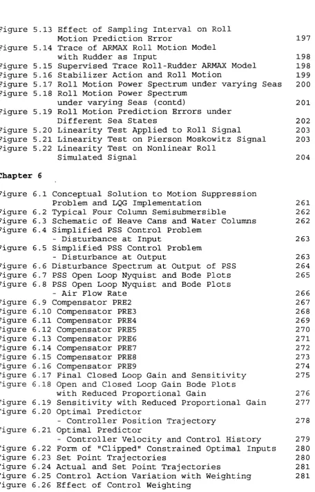
Figure 4.5 Parameter Estimates (PM) 1-Step Predictor 134 Figure 4.6 Parameter Estimates (PM) 3-Step Predictor 135 Figure 4.7 Parameter Estimates (PM) 7-Step Predictor 136 Figure 4.8 Predicted and Actual PM Signal 137 Figure 4.9 Predicted and Actual PM Signal 138 Figure 4.10 Autocorrelations of Prediction Errors

Distance= Optimal 1, 1, 2 Steps 139 Figure 4.11 Autocorrelations of Prediction Errors

Distance= 3, 4, 5, and 6 Steps 140 Figure 4.12 Autocorrelations of Prediction Errors

Distance= 7, 8, 9, and 10 Steps 141 Figure 4.13 Mean Square Errors using Concatenation

to Generate Multistep Predictions 142 Figure 4.14 Mean Square Errors using "Hybrid"

Concatenation to Generate

Multistep Predictions 142

Figure 4.15 Mean Square Errors using Recursion of

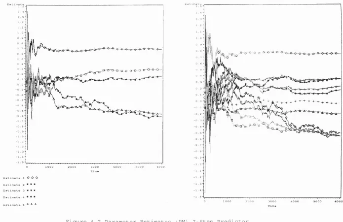
Diophantine to Generate Multistep Predictions 143 Figure 4.16 Filtered Pierson Moskowitz Spectrum 144 Figure 4.17 Mean Square Errors T=6 PM Filtered Signal 145 Figure 4.18 Autocorrelation of Prediction Errors

T=6 PM Filtered Signal 146

Figure 4.19 Parameter Estimates T=6

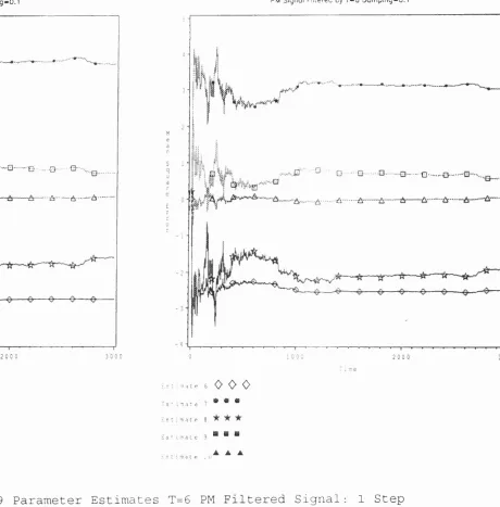
PM Filtered Signal: 1 Step Predictor 147 Figure 4.20 Parameter Estimates T=6

(11)

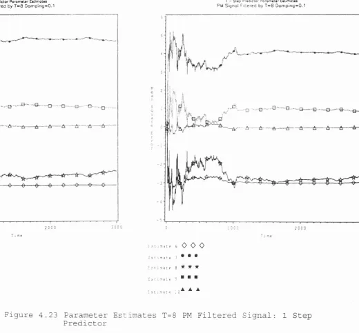
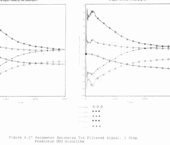
Figure 4.23 Figure 4.24 Figure 4.25 Figure 4.26 Figure 4.27 Figure 4.28 Figure Figure Figure 4.29 4.30 4.31 Figure 4.32 Figure Figure 4.33 4 . 34 Figure Figure Figure 4.35 4.36 4.37 Figure Figure 4.38 4.39 Figure 4.40

Chapter 5

Figure Figure Figure Figure Figure Figure 5.1 5.2 5.3 5.4 5.5 5.6 Figure Figure

5 . 7 5.8 Figure 5.9 Figure Figure 5.10 5 .11 Figure 5 .12

Parameter Estimates T=8

PM Filtered Signal: 1 Step Predictor Parameter Estimates T=8

PM Filtered Signal: 3 Step Predictor Autocorrelation of Prediction Errors T=8 PM Filtered Signal

Mean Square Errors T=6

PM Filtered Signal: UDU Algorithm

Parameter Estimates T=6 Filtered Signal : 1 Step Predictor UDU Algorithm

Parameter Estimates T=6 Filtered Signal: 3 Step Predictor UDU Algorithm

Error (PM Pole System) and Barge Signal Forgetting Factor Effect on

Mean Square Errors - PM Signal

Mean Square Error - Constant Dynamics Mean Square Errors

-Dynamics Change at T=1000 Sum of Mean Square Errors

Fortescue Variable Forgetting Factor Mean Square Errors with

Variable Forgetting Factors

Modified Variable Forgetting Factors Trace of Covariance Matrix with

Modified Forgetting Factors

151 152 153 154 155 156 157 157 158 159 160 161 162 162 163 164 165 166

Ship Roll Motion

Ship Roll Motion Power Spectrum Ship Roll Motion Autocorrelation Roll Motion Crosscorrelations Rudder Action

Effect of Model Order on Roll Motion Prediction Error

Ship Roll Motion Mean Square Prediction Errors Roll Motion Predictor Parameter

Estimates 1-Step

Roll Motion Predictor Parameter Estimates 3 -Step

Errors Distance= 3, 4, 5, and 6 Steps Autocorrelation of Ship Motion Predict;

(12)

Figure 5.13 Figure 5.14 Figure Figure Figure Figure 5.15 5.16 5.17 5.18 Figure 5.19 Figure Figure Figure 5.20 5.21 5.22

Motion Prediction Error with Rudder as Input

Chapter 6

Figure 6.1 Figure Figure Figure 6.2 6.3 6.4 Figure 6.5 Figure Figure Figure Figure Figure Figure Figure Figure Figure Figure Figure Figure Figure Figure Figure 6.6 6.7

6 . 8

9 10 11 12 13 14 15 16 17 18 6.19 6.20

Figure 6.21 Figure Figure Figure Figure Figure 22 23 24 25 26

under varying Seas (contd)

Roll Motion Prediction Errors under Different Sea States

Linearity Test Applied to Roll Signal

Simulated Signal

Conceptual Solution to Motion Suppression Problem and LQG Implementation

Typical Four Column Semisubmersible

Schematic of Heave Cans and Water Columns Simplified PSS Control Problem

- Disturbance at Input

Simplified PSS Control Problem - Disturbance at Output

Disturbance Spectrum at Output of PSS PSS Open Loop Nyquist and Bode Plots PSS Open Loop Nyquist and Bode Plots - Air Flow Rate

Compensator PRE2 Compensator PRE3 Compensator PRE4 Compensator PRE5 Compensator PRE6 Compensator PRE7 Compensator PRE8 Compensator PRE9

Final Closed Loop Gain and Sensitivity Open and Closed Loop Gain Bode Plots with Reduced Proportional Gain

Sensitivity with Reduced Proportional Gain Optimal Predictor

- Controller Position Trajectory Optimal Predictor

- Controller Velocity and Control History Form of "Clipped" Constrained Optimal Inputs Set Point Trajectories

Actual and Set Point Trajectories

Control Action Variation with Weighting Effect of Control Weighting

(13)

Figure 6.27 Figure 6.28 Figure Figure 6.29 6.30 Chapter 7 Figure Figure Figure 7 .1 7.2 7.3 Figure Figure Figure 7.4 7.5 7.6 Figure Figure 7.7 7 . 8 Figure 7.9 Figure 7 .10 Figure Figure Figure Figure Figure 7 .11 7 .12 7.13 7 .14 7.15 Figure Figure Figure Figure Figure 7.16 7 .17 7.18 7.19 7.20 Figure 7.21 Figure 7.22 Figure Figure 7.23 7.24 Figure 7.25 Figure 7.26 Figure Figure 7.27 7.28

on Trajectory Behaviour Effect of Control Weighting on Trajectory Behaviour

Trajectory and Control Behaviour for Predicted Time Varying Setpoint

Point Attractor for Various Values of Damping Five Coexisting Periodic Steady States

Hayashi Catchment Regions for Harmonic and Subharmonic Motion of Order 3

Chaotic Motions of Nonlinear Oscillator Trajectory Divergence of Adjacent Starts Control Space of Duffing's Equation

as determined by Ueda Liapunov Stability

Phase Behaviour and Stability Regions of a Continuous Linear System

Poincare Sections off Three Dimensional State Space

One and Two Dimensional Poincare Sections of an Autonomous Flow

Discrete Time Routes to Instability Tracking of an Evolving Linear System Damped Fold Time History

Undamped Fold Time History

Instability Predictions Based on

Frequency Evolution of the Undamped Fold AR Model Parameters Order 3, Undamped Fold System and Model Outputs

AR Model Parameters Order 5, Undamped Fold Fold with N( 0,0.5) Additive White Noise Input A R M A (2,2) and A R M A (3,3) Models Fitted

to Noise Driven Fold

Phase Portraits for Supercritical(Stable) and Subcritical(Unstable) Hopf Bifurcation Schematic of the Stable and Unstable Hopf Bifurcations

Supercritical Hopf Time History Supercritical Hopf Disturbed by N ( 0,0.5) Noise Input

A(z'^) Parameters of A R M A (3, 3) Model for Disturbed Hopf

Tracked Damping in Evolving Hopf with Additive Noise

Experimental Model of a Moored Vessel Displacement Time Histories for

(14)

Figure 7.29 Displacement Time Histories for Evolving System

Figure 7.30 Estimated Damping as a Function of Mooring Arm Length

Figure 7.31 Experimentally Determined Bifurcation Diagram Figure 7.32 Damping Estimation for Evolving System

on Equilibrium

326 327 327 328

Chapter 8

Figure 8.1 Figure 8.2

Figure 8.3 Figure 8.4 Figure 8 .5 Figure 8 .6 Figure 8 .7 Figure 8 . 8 Figure 8 . 9

Poincare Points and Spectral Components for Bilinear Spring with White Noise Poincare Points and Spectral Components for Bilinear Spring with

Frequency Wandering Noise

Poincare Points and Spectral Components for Bilinear Spring with Bandwidth Noise Maxima and RMS Values for Three Types of Randomness: Bilinear Spring

Time History of Bilinear Spring under Different Forcing

Poincare Points for Mathieu System with White Noise

Poincare Points for Mathieu System with Frequency Wandering Noise

Poincare Points for Mathieu System with Bandwidth Noise

Maxima and RMS Values for Three Types of Randomness: Mathieu System

(15)

Chapter 1 Introduction

1.1 Trends in Offshore Structure Design

with the advent of newer types of offshore structures designed for deep waters and hostile environments increasing emphasis has been placed on the dynamical behaviour of offshore structures. Early practice was largely limited to the design shallow water oil production platforms such as steel or concrete gravity structures using principally static methods of analysis. The design of ocean structures like that of ships has been based partly on empirical codes and rules that rely on well learnt past experiences. The major concern in the design of an offshore structure is to ensure that the natural period of vibration is distinct from the period of expected waves (Langewis 1986). The severe limitations of designs based on linear models in possible operational situations was not fully recognized.

(16)

stresses by moving in a compliant, yielding manner with the waves and current. Large displacements are a feature of compliant structures such as tension leg platforms (TLP) , moored semisubmersibles and articulated mooring tower. The large working displacements imply that the dynamics can be expected to be inherently nonlinear. Indeed assumptions of near linearity are often inadequate for a reasonable prediction of extreme response

(Thompson et al (1984a).

The size of some of these compliant structures is impressive / the Hutton tension leg platform (TLP) for example weighs about 50,000 tonnes with a deck larger than a football pitch. The magnitude of these structures implies that even small improvements in the design may give large savings in construction costs. In a passive design if predicted displacements caused by environmental and operational loads are too large it is usual to reduce the coupling between force and structure by a change of geometry or to increase the stiffness of the structure to raise the natural frequency above the excitation frequency.

1.2 Active Control for Motion Suppression

(17)

because of the lightly damped dynamics of the structure and primarily because of the uncertain exciting wave and wind force disturbances of changing sea states and weather. In a real sense it is the random disturbances that cause the control problem and the nature of the disturbances has a direct influence on the difficulty of control. Feedback is an effective means of coping with uncertainty such as uncertain disturbances, dynamic parameter variations and nonlinearities.

The benefits of active control systems are widely recognized in the aerospace industry. The Lockheed Tristar for example uses wing tip accelerometers to control ailerons to minimise wing root bending stresses and hence extend the structures fatigue life with negligible weight penalty. There has been some work in the onshore civil engineering field on the control of bridges and buildings (Leipholz 1980) .

Dynamic ship positioning (Grimble et al (1980)) is a well known example of the use of feedback control in the ocean engineering field. Thrusters control mean position more conveniently and cheaply than could a passive mooring system, since conventional moorings or anchors are not required and no costly delays are incurred due to laying and retrieving anchors. In this problem the system dynamics need only be known to optimise the removal of the wave frequency motions from the position signal. Only the low frequency motions are suppressed since the thrusters have insufficient power to overcome the high frequency wave forces. The control of zero or low frequency motions of rig ships, submarines is an active and mature field that could possibly be improved by the adoption of adaptive techniques. Linfoot et al

(1982) consider control systems to suppress the low frequency motions of single point moored (SPM) vessels.

(18)

compliant and stiff modes of compliant structures and the slowest modes of stiff structures offer potential applications and will result in lower fatigue damage and/or wider operating windows. General design tools and techniques for the active and adaptive

control of marine structures are investigated.

1.3 Adaptive Motion Prediction

Intimately related to the problem of control is the problem of predicting the motions of wave driven compliant structures . A reliable predictor of the future motion of a ship or barge under the influence of random wave and wind forces would have a variety of applications in the control of aircraft or helicopter landing, cargo transfer aboard ships, structural installation and floating crane operations in rough seas. For example the safe landing of aircraft on board small vessels is a most delicate phase of flight operations at sea. If predictions of the future motion of the vessel were known within reasonable error bounds one could expect a significant improvement in touchdown windows and a reduction in the number of waveoffs. Much of the previous work in this area (Sidar and Doolin (1983), Lincoln (1983), Triantafyllou (1982)) has assumed that an accurate model of the vessel dynamics is known and furthermore that a differential equation representation of the exciting force spectrum exists. The ships equations of motion are transformed to state space form and a Kalman filter implementation is used to generate predictions. Details of the exciting force spectrum depends on the wave directionality, orientation and speed of the vessel. Even when the directional wave spectrum is known it is not simple to evaluate the spectrum of the exciting force and hence derive a differential equation model (Maciejowski (1983)). An adaptive approach (Goodwin and Sin (1984)) to the prediction problem is clearly warranted because of the time varying dynamics and random disturbances.

(19)

Jenkins (1976)) is formulated as an analogous problem to that of designing a minimum variance self tuning controller (Astrom and Wittenmark (1973)). The predictors abilities are assessed and possible uses of predictions as an operator guide and methods of direct incorporation of predictions within a control loop are developed.

1.4 Prediction of Extreme Responses

(20)

system identification techniques to track nonlinear systems evolving towards a bifurcation in the presence of noise are evaluated.

1.5 An Outline of the Thesis

This thesis is concerned with how real time prediction and control techniques can be used to mitigate the problems caused by the motions of compliant marine structures subject to random wave and wind forces. The structure of the thesis is outlined below

Chapter 2 The question of why a random signal can be predicted

and the inherent assumptions is addressed. The general theory of linear prediction is developed from a state space viewpoint and the algorithmic details of the Kalman filter and prediction from state space models is reviewed. The Autoregressive Moving Average (ARMA) based representation is derived and shown to be equivalent to a canonical representation of the Kalman filter in an innovations form. Various control interpretations of the prediction problem are given.

Chapter 3 The important areas of system identification and in

particular parameter estimation are highlighted. The relationships between the well known recursive least squares (RLS) and extended least square(ELS) to Kalman filtering is shown. Theoretical modifications necessary for adaptive systems are discussed with particular relevance being given to variable forgetting factor schemes. The self tuning predictor is introduced and a proof of optimality given.

Chapter 4 Simulations of various test signals are used to assess

(21)

Chapter 5 Real ship motion data is used to give the self-tuning predictor a sterner test than the previous simulations. The possibility of using auxiliary inputs and nonlinear functions of past roll history are explored. The usefulness of the predictor algorithm as an operator guide to assist in helicopter landings is evaluated. A simple test is presented for linearity and an algorithm is suggested for further work.

Chapter 6 The state space model of a conventional semisubmersible

with pneumatic heave suppression cans is derived and a suppression controller is developed in the frequency domain. The practical feasibility of the scheme is assessed . The use of predictions in a control scheme is explored and an optimal prediction formulation is given for a crane-barge loading system. The importance of constraints is emphasized and a model based predictive scheme is introduced as an efficient control design strategy that can incorporate constraints in a transparent manner.

Chapter 7 The richness of nonlinear systems is illustrated. The

presence of significant nonlinearities in the dynamical equations of offshore structures can under regular sinusoidal excitation give rise to disturbingly large subharmonic or chaotic motions. System identification techniques together with ideas from catastrophe and bifurcation theory are used to predict incipient dangerous excursions of compliant marine structures subject to regular forcing. An experimental study of a fishtailing tanker illustrates further some of the developments.

Chapter 8 The persistence of the subharmonic motions of the

nonlinear marine structures subjected to various types of random forcing is examined. Time domain simulations of the equations of motion are used to explore the response of the nonlinear systems to random inputs. The prevention and control of the bifurcational behaviour of a system to nonbifurcational behaviour

(22)

CHAPTER 2 Linear Models and Prediction

2.1 Introduction

The desire to predict the future is the universal driving force behind the search for laws that explain the behaviour of both man made and natural systems,(Whittle 1984). Examples include the anticipation of financial stocks and shares, to forecasting the weather.

The ability to predict the future evolution of a given system depends on two types of knowledge. "White" knowledge that is based on rigorous models of the underlying physical laws of the phenomena is the first and most powerful type of knowledge. Such knowledge can be expressed in the form of equations that can in principle be solved. Given the initial conditions ,to infinite accuracy for chaotic systems (Lorenz 1964),the future can be completely predicted. The construction of an accurate rigorous can model can however be extremely difficult for most real physical phenomenon and impossible for many more. Recourse must often be made to approximations, that lead to a "tractable" mo d e l .

The second approach is the "Black Box" method, that relies on the elucidation of strong empirical regularities in the observations of a system.

To introduce the basic concepts involved in prediction it is instructive to consider the prediction problem first in a deterministic framework.

2.2 Prediction in a State-Space Framework

(23)

equation descriptions an extra set of variables is used to take account of the past history of the system; these are the so called state variables of the dynamical system. Such state space descriptions are commonly used in modern control theory (Dorf 1980) in which the basic form of description of a dynamical system is comprised of relationships between three sets of system variables : input, output and state variables. The state variables are functions of themselves and the input variables, that is the values of the state variables are associated with sets of functions of time which define the past behaviour of the inputs and of the states.

If the elements of the input vector u e , is a set of input variables and the set of state variables is given by the elements of the vector x e i?" , then using integration as the simplest possible functional relationship in which to express the present in terms of the past, the j th state variable may be found as

Xj{t)

= j

^ j{x, u, t) dt (2.1)

Where the set of functions 0^- define the nature of the system dynamics as summarised in the current values of the states.

Equation (2.1) clearly implies that the state variables satisfy a set of first order differential equations

X. ( t) = 0 . (x, u, t) j = 1, . . .n (2.2)

Surprisingly most (Derusso 1965) physical systems can be described with a simple form of 0j in which the effects of the states and inputs are separated. Indeed modern controller design depends heavily on this separation in the design of algorithms. Equation (2.2) can then be written as

(24)

To complete the standard state space model an output vector y e

Rf" is obtained from the set of input and state variables as

y^{t) = {x, u, t) i = 1 .m (2.4)

Once again in most real systems the effect of the states and inputs can be separated to yield

y^ ( Ü) = 0 j (x, t) + |i^ (u, t) i = 1, . . .772 (2.5)

The standard state space model then takes the form

x(t) = f(x,t) + g{u,t) (2.6)

y it) = 6 (x, t) + |i (u, t)

Where f,g,S and fj, are vector functions of the appropriate dimensions.

Restricting analysis to linear systems (Kalman 1963) the state space model assumes the form

x(t) =A(t)x{t) +B{t)u{t) y{t) = C(t)x(t) + E(t)u{t)

Where _(2.7)

x{t) 6 A(t) e R ^

u{t) Ç R^ Bit) €

y{t) E R^ C(t) E

E{ t) E

For time invariant systems further simplification is possible

x(t) = Axit) + Bu(t) (2.8) y it) = exit) + Eu it)

(25)

the state vector is not a unique set of variables and in fact any- set related by a nonsingular linear transformation (Luenberger 1967) of the form

it) = P x{ t)

gives an equivalent input-output description. The matrix A is the dynamical or state map and represents the internal physical mechanism by which the state evolves and by which energy is converted and dissipated within the system. Matrix B is the input or actuator map and represents how the system is affected by the environment. The matrix C is the output or sensor map and represents the way in which information about the system is conveyed to the environment. Finally matrix E is the direct coupling between input and output, in the sequel E . ±s assumed zero, since for mechanical systems such direct coupling is physically unlikely.

Once a state space realization of the dynamical behaviour of a system has been found the prediction problem is then equivalent to finding a solution to the matrix differential equation. The solution to (2.7) can be shown to be (Derusso 1965)

x{t) = [X( t ) t g ) ] x( t g ) + f ^ X( t ) (t ) B (t) u (t) dx

(2 .1 0 )

y it) =

at)

x{

t)

Where X(t) is a fundamental matrix containing a basis set of n

linearly independent solution vectors as its columns. From the independence of the solution vectors, X(t) is always of full rank and thus possesses an inverse X'^ (t) defined at all times . Defining the transition matrix and rewriting equation (2.10)

0 ( t,x) = X{t)X-^(x)

x{t)

=

0 (t,tg)x(tg)

+

J'

^

0

( t, t) B(z) u(z) dr

, (2 .1 1 )

(26)

given by

X{t) = exp {At)

(2.1 2)

This follows since

d

[exp(y^t)] =^exp(^f)

dt - ' (2.13)

exp {A.Q) = J

Equation (2.10) may therefore be written as

x{t) = [exp A ( t-Üq) ] x( Üq) + exp[A(t-T)] Bu{x) d'z

•'to (2.14)

y{t) =C x{t)

Where x(to) is the initial value of the state. The physical interpretation of the input-output relationship can be seen if the input is considered as a stream of impulses.

An impulse input of magnitude ot at time r

u{t) = a ô(t-T) (2.15)

causes a discontinuous state jump of amount

x(T + ) - x ( T - ) = B a (2.16)

So that if the impulsive input is applied to a quiescent system it will kick the state from zero to Ba , the subsequent motion will therefore be the same as would result from the release from an initial state value

x{x) = Ba (2.17)

The evolution of the state is using the transition matrix

x{t) = exp[A(t-T)] .Ba

(27)

In the limit form an impulsive stream of inputs starting at t=0

can be represented as

u{t) = f ^u (t) Ô ( t-x) dT (2,19)

JQ

It is clear then that the output consists of a free motion part

y free = C e x p [ A ( t - t g ) ] X ( to ) ( 2 . 2 0 )

and a forced motion part

yforced(^) = C exp [^( t-T) ] Eu(x) dx (2.21)

which is the limiting sum of responses from the set of initial conditions into which the impulse input stream successively kicks the system.

Equation (2.14) shows that given the state vector at any particular time, and the sequence of future inputs one can extrapolate and determine the future evolution of the state vector and hence the output y (t) .

If for example u(t) is a zero mean white noise process (Papoulis 1965) which by definition is completely unpredictable, and the state at time t is x(t) then it follows that the only predictable part of the output and state evolution is given by the free motion term as

x { t + T / t ) = exp [a(r) ] x( t)

(2 .2 2 )

vit + T/t) = C x(t+Tjt)

For a deterministic system in free motion, the future motion would be uniquely determined by the actual value of the state.

(28)

y {t) + ca^y ( t) - f ( t) (2.23)

Where f(t) is the forcing term.

The equations may be expressed in state space form by defining

=

y

(0

So that

y

^ 0) (0 (0 0)

Xg ( t) = y it) = o)x^ ( t)

f2.24j

Rewriting in matrix form

( t)

x^it)

y{t) = \ 0 1 I

0 — (i) %i(k) 1

+

0) 0 x^it) 0

x^ ( t)

X2(t)

f ( t) (Ù

(2.25)

(29)

0 -(Ù t 0

At = A^t^ =

0) t 0 0

z2f-2

= I + At + — + .

2 ! = @(C,0

cos (ùt -sin cot sin 0) t cos to t

(2,26)

The free motion response to arbitrary initial conditions is therefore

x{ t+T) = 0 ( r, t) x( t)

y{C+T) = sin (ùiT)Xj^(t) + cos (ù {T) x^it)

(2.27;

2.2.1 Linear Systems Driven By Stochastic Inputs

In order to predict the output of a system driven by a stochastic input signal a differential equation representation of the disturbance must first be found. This is essentially the internal model principle of Francis and Wonham (1976), which states that before one can predict or control a system a model of the system and environment with which it interacts is required. The correlation between the random disturbance inputs will in general, be specified by the spectral density matrix and the problem is then to determine a characterization of the disturbances in the time domain. The stochastic disturbance is modelled by introducing a fictitious linear dynamic system which is itself excited by white noise. The states of the disturbance model are then augmented to the system states to give an enlarged A matrix. Stochastic realization theory which shows how to fit systems to spectra is discussed in Davis and Vinter (1985) , Maciejowski

(30)

specification of the linear system and variance of the driving force. Consider a disturbance signal d(t) with spectral density

then Dj must be chosen so that

Where

x^it) = A^^it) + B^w(t)

(2.28)

dit) = D^^it)

The disturbance states x^(t) do not correspond to physically measurable quantities and are simply a means of converting the white noise input w(t) into a signal d(t) with the required spectral density.

Augmenting the disturbance states with the original system equations denoted with subscript s here for clarity yields

0 +

^d

w

0 A^ _^d

y ( t ) = |c^ o|

(2.29)

Rewriting in a compact form with x(t) = [x^(t) Xj(t)]’’'

x(t) = A^(t) + B^w(t) y(t) = C^it) = C^^(t) (2.30)

Since w(t) is a white noise process the only predictable part of the state evolution is given by the free motion term in the solution to equation (2.30). The optimal prediction is therefore given by

xit+T/t) = exp [A^(T) ] x( t)

(31)

Summarising it is apparent that both system and disturbance dynamics form the basis of prediction. Prediction quality will decay with time due to the fact that the unpredictable white noise input term influences more and more of the future behaviour of the system. The ability to predict is governed by the undriven combined system and disturbance dynamics and the availability of an initial state vector x(to) measurement.

For a complex system the state vector may be of a high dimension and in general not all elements of the state vector will be available for measurement. This may arise because of cost constraints on instrumentation or the fact that certain states correspond to obscure internal quantities that cannot be measured. Furthermore the disturbance states in (2.29) cannot be measured anyway since they are simply an artifact of the modelling. The state vector therefor must be reconstructed using observers (Luenburger 1967) or optimal estimation techniques (Kalman 1960). Once a state estimate is obtained the prediction is obtained by extrapolating the state estimate in time using the system transition matrix.

2.3 State Reconstruction: The Kalman-Bucy Filter

If the signal to be predicted y(t) is assumed to be modelled as the output of a linear stochastic model as above, a solution to the state estimation problem can be obtained using the Kalman filter (Kalman and Bucy (1961)). Generalising equation (2.30) to include a corrupting random vector noise on the output gives

x(t) = A^{t) + B^w{t) (2,32)

yi t) = C ^ ( t) + v{ t)

Where w(t) is a white vector random process with zero mean and covariance matrix

cov [w{t) ,w{x)] = Qb{t-'z) (2.33)

(32)

a white stationary zero mean process with covariance matrix

cov [v{t),vix)] = R à i t-x) (2.34)

Stationarity of the noise process which means its properties are time invariant, is assumed for convenience, the non stationary case can also be easily handled.

The initial state vector is assumed to be a vector random variable with zero mean and uncorrelated with the noise so that

cov [x H q) , wit^) ] = 0 cov [x( to) , v( tg) ] = 0 (2.35)

The estimate x(t/.) of the unknown state x(t) is to be optimal in the following defined sense. If the state estimate error is

x(t) = x(t) - x ( t / .) (2.36)

then the estimate must be unbiased ,that is

E [x(t/.)] = E [x(t)l (2.37)

and the estimation error (2.36) must have minimum variance

E [x"^(t)x(t) ] = Error Variance (2.38)

The covariance matrix of x(t) is defined as

E [x{t)x^(t)] = Pit) (2.39)

For the stationary time invariant case the error covariance matrix P(t) converges to a steady time invariant matrix P (Bryson and Ho (1969) ) and it can be shown that the optimal linear unbiased estimate with minimum error variance can be realized by the feedback system of the form shown in Figure 2.1.

The optimal state estimate is then given as

x( t / .) = Ax(t/.) + K [y(t) - Cx(t/.)] (2.40)

(33)

K = PC^R~'^ (2.41) P is the steady state covariance matrix of the state error

P = cov [x,x'^] (2.42)

and is the solution of the algebraic Ricatti equation

AP + PA"^ - PC^R-^CP + BQB'^ - 0 (2.43)

Since P is a covariance matrix it must by definition be positive definite. For a state vector of dimension n the Ricatti equation gives n(n+l)/2 quadratic equations for the unknown elements of P so that there is in general no unique solution for P.

Intuitively the existence of a solution to the optimal filtering problem depends on the observability (Kalman 1963) of the pair

[A,C] which implies a nonsingular solution for P. Furthermore it

can be shown (Martensson (1971), MacFarlane (1963)) that subject to the observability of the pair [A,C] there always exists a unique positive definite solution. Details of numerical methods to find solutions to Ricatti equations are discussed in Laub

(1979) .

2.4 Discrete Time Formulation

In practice state estimation and prediction would be carried out in discrete time. The discrete time formulation of the Kalman filter therefore has a practical relevance to implementation. Transformation from continuous time to discrete time is easily facilitated (Franklin and Powell (1980) ) using the transition and impulse response matrices derived from solution of the continuous time equations.

If for the continuous time system interest is focused on the system state at discrete evenly spaced points in time

x{t) =A(t)x(t) +B{t)u(t) +G(t)w(t) (2.44)

(34)

then the resulting difference equation is

x(ic+l) = O^(ic) + Aj^uik) + T^w(k) (2,45)

Where ^ is the transition matrix and tjt)

Tj^wik) = ^ G(t) w(t) dz ^2 4^;

Aj^ u{k) = ^ z) B(z) u(z) dz

Note that the equations (2.46) does not uniquely define the terms

u (k) , w (k) but only the product terms T]^w(k) and A^u(k). If

a zero order hold is assumed for the deterministic input so that

uiz) = u{k) ty. <T< (2.47)

Then

Ay = z) B(z) . dz (2.48)

The random forcing function can be defined in terms of the covariance matrices so that for the forcing function G(t)w(t) the covariance matrix is

E [G{t) w{t) {z) G~^ {z)] = G{t) Q{t) G'^ it) b (t-z) (2.49)

In the discrete time formulation the corresponding covariance matrix is given by

[(r^i^(ic)) (r,u.(i)) = T y Q ^ l k = i ^2 .5 0)

= 0 k * 1

From equation (2.46) and (2.50)

ryOj^l ( ty^^,z) G{z) w{z) w^{a) G'^(a) dzda

(35)

Using (2.44) this becomes

= /■''*•' $(t;,.l,T)G(T)C)(T)G^(T)<&^(t*.i,T)dT (2.5 2)

•'tjt

The assumption of stationarity for the random process w(t) and time invariant dynamics simplifies the above equations so that for a sampling interval of T

^ = F = exp [AT]

= A = J ^exp [A(T -t) ] dt (2.53)

The random forcing terms fkj can be replaced by a noise sequence e (k) with covariance matrix

E{ee'^) = r p r^ = f ^ exp [A{T-z)] GQG ^ exp ^(T- 1) ] dt

Jo

(2.54)

The stochastic state space model in discrete time can then be written as

x{k+l) = Fx{k) + ru(ic) + e{k) 5 5)

y{k) = Cx{k) + v{k) ( ' /

Noise sequence v(k) is found using the same method as for e (k) .

The model (2.55) describes the evolution of the state and output in terms of probability distribution functions. For example the probability distribution of the state in terms of its mean and covariance is given by the recursive equations

x{k) = E[x(k) ]

P{k) = E[ (x{k) - x{k) ) {x{k) - x{k) )

x{k+l) = Fx{k) + Au{k)

P(k+1) = FP{k) F'^ + TqT'^

(36)

S t a t e x(0), b u t may be cross correlated so that

E e{k)

v{k) \e{k) v{k)\ =

= 0

s

R (2.57)

The discrete form of the Kalman filter can be stated as follows (Bryson and Ho (1969)). Let x(t+l/t) denote the conditional mean

of x(t+l) given observations of the output sequence { y(t) } up

to and including time t.

x{t+l/t) = E[xit+1)/Y(t)]

Y{ t) = {y( t) ,y( t-1) , . . .} (2.58)

Then the optimal linear unbiased minimum variance estimate of the state satisfies the following recursion

x{t+l/t) = Exit/1-1) + K^[y{t) - Cx{t/t-l)] + Au(ic)

(2.59)

is the Kalman gain that is given by

Kf. = [FP^C^ + S] [CP(.C^ + i?]

Pt is the state error covariance at sample time t

(2.60)

P^ = E[{{xit) - x{t/1-1) ) ix{t) - xit/t-1) ) ^/iy{t-l)

(2.61)

and satisfies the following Ricatti difference equation

= FP^F'^ + rpr^ - JCjCPf.C^ + R]Kt^ (2.62)

Implementation of the filter involves solving the discrete Ricatti equation for the sequence P^. and the corresponding gain matrices K,.. These calculations can be done off line before any observations are taken and used to recursively update the state estimate x(t/t-l) as observation data becomes available.

The Kalman filter equations may also be recast into a form in

(37)

which the cross covariance term

S

(2.57) may be taken as zero. Any crosscorrelation present is included in a modified

Q

matrix, details may be found in Bryson and Ho. In the sequel

S

is assumed zero.

For the case of linear time invariant system and measurement dynamics and stationary noise processes, the filtering process will reach a steady state. The error covariance matrix and hence the Kalman gain converge to steady state values with increasing time ; the limiting solution P will satisfy the following algebraic Ricatti equation, derived from (2.62) by putting Pj,^^=Pj,=P

P - FPF^ + FPC^iCPC^ + R)-^CPF'^ - = 0 (2.63)

With steady state gain matrix K

K ^ FPC'^iCPC'^ + R)-^ (2.64)

Various theorems (Kalman (1963),Bryson and Ho (1969)) give the limiting properties of the Kalman filter under a number of conditions and are important in establishing sufficient conditions for the asymptotic time stability of the filter. The results are centred around the observability of the pair [F,C]

and stabilizibility of the pair [F,D] where D is a factor such that

DD ^ = VqV^ (2.65)

The Kalman filter has a number of interesting interpretations that will be used to motivate further developments. In a Bayesian (Papoulis (1963)) framework consider the problem of finding a state estimate x(./.) to minimise the generalized minimum variance cost functional

J =

f f ...f

(3t-x) '^T{^-x) p{x,

{Y})

dx^dx^. . .dx^ (2.66)

Jo Jo

Jo

Where

(38)

p(x/{ y}) is the conditional density function of the state given past and present observations.

Setting dJ/dx = 0 gives that independent of T (Gelb 1982)

^ ^ fo fo ’ ‘ ’fo ^ ) dx^ . . .dx^ = E[x/ { y} ] (2.67)

The optimal estimate is therefore the conditional mean estimate. For linear systems driven by Gaussian white noise processes the Kalman filter can be shown to generate the state estimate x(t/t-1) as the conditional mean of x(t) given {y(t) ,y(t-1)...}.

x(t) = E[x(t) / Y(t-l) ] (2.68)

The Kalman filter is a recursive and hence efficient solution to the problem of computing the conditional probability distribution. The minimum variance property for the estimate of

X clearly follows from (3.66), furthermore

E[{x{t) - x{t) ) / Y{t-1) ] = 0

(2.69)

Pf. = E[{:^{t) -x{t)){Jt{t) - x( Ü) ) V y ( t-1) ] ^ Pt

Where P° is the covariance given by any other filter, linear or nonlinear.

For non Gaussian noise processes the filter gives the best linear minimum variance estimator, the estimation error is however still uncorrelated with past data so that

E [ (xit) - x(t) ). Y(t-i) ] = 0 2= 1,2 ... (2.70)

Equation (2.70) can be used to motivate a geometric interpretation of the state estimate , in which the best estimate

of x(t+l) is the projection of x(t) onto the linear space

(39)

0) ( t) = vit) - Cx{t) (2.71)

Since this term contains the "information" on which the filter works. The sequence { b (t) j is called the innovations (Kailath 1968) sequence since ^ (t) represents new information available at sampling instant t. From (2.70) it is apparent that the innovations are orthogonal or uncorrelated with the past values, so that

( t)/Y{ t-1) ] = 0 (2.72)

Using the innovations the output y(t) of the system may be written as

y(t) = exit) + 0) ( t) (2.73)

The state estimation equations may also be recast to give

x(t+l) = Fx(t) + Auit) + K^(ù{t) (2.74)

Clearly the innovations model as described by (2.73) and (2.74) represents an alternative input-output state space description of the original system. Indeed it can be shown that to every state space model there corresponds an "equivalent" innovations model (Luenberger 1967) . It therefore follows that the innovation models are just as rich as state space models in representing the input-output behaviour. The innovations model however includes fewer parameters and a reduced number of noise inputs. Furthermore an alternative predictor derivation is easily facilitated using the innovations representation.

2.4.1 Prediction Using the Discrete State Estimate

Examination of (2.74) reveals that the Kalman filter actually corresponds to the one step ahead state prediction

(40)

The optimal d step ahead prediction corresponds to the conditional mean E [x (t+d) /y (t) ,y (t-1) , . ] . The so called smoothing property of conditional expectations (Goodwin and Sin

(1984) ) can be used to write

E[x{t+d) /Y{t)] = E{E[x{t+d/Y{t+d-l)] /Y(t)}

(2.76)

= E[^{t+d) /Y{t) ]

From (2.74)

t+d-l t+d-l

x{t+d) = t+1) + ^ Au(j) + ^ ij)

j=t+i j=t+i

(2.77;

Taking expectations of (2.77) conditioned on data up to time t and using equation (2.72) yields

t+cf—1

E[x{t+d)/Y{t)] = F^-^x(t+l) + F^*^-^-^Au{j) (2.78)

j=t+i

and this is from (2.76) equivalent to E[ x(t+d)/Y(t)] . The corresponding d step ahead prediction of the output y (t+d/Y(t) )

is simply obtained as

t+cf~l

£'[y( t+d)/y( t) ] = CF‘^'^x(t+l) + C Y (2.79)

j=t+i

2 . 5 Autoregressive Moving Average (ARMA) Representation of

Stochastic State Space Models

An alternative and often more convenient way of describing the input-output behaviour of the stochastic state space model is by the Autoregressive Moving Average model with exogenous input, ARMAX model (Box and Jenkins (1973)) .

Consider an r dimensional vector output y(t) and an m

(41)

y(t) + A^y{ t-1) + . . .A^{t-n) = B^u{ t-1) +...B^u{t-n)

+ e{t) + C^e{ t-1) .... C^e( t-n)

A{z ^)y(t) = B(z ^)u(t-l) + C(z ^)e(k)

(2.80)

Where

Aj... .A„ are r x r matrices

. . . . are r x m matrices

. . . . Q are r x r matrices

and {e(t)} is a sequence of zero mean uncorrelated r dimensional

vector random variable. An equivalent state space representation will always exist , such that

-Ai I q -A,

x{t+l) =

: 1 x{ t) + u(t) +

-A, 0 _Bn _Cn

-e ( t)

(2.81)

y(t) = |J 0 - 0|x{t) + e{t)

A state space representation with this structure is called the "observer" form (Luenberger (1967)).

For example for a single input single output (SISO) stochastic state space model in observer form the corresponding innovations model is

-a± 1 _K

x(t+l) =

: 1 x{ t) + u{t) +

-3% 0 bn K

(*) ( t)

(2.82)

(42)

From the multi input multi output (MIMO) form above or by direct substitution the corresponding ARMAX model for a single input single output (SISO) system is

y(t) + a^^yit-l) +...a^y{t-n) = b^u{t-l) + . . .b^u(t-n)

+ (Ù {t) + [ + ic^] (*) ( t-1) + ... [a^ + ic^] Ù) ( t-n)

(2.83)

If the Kalman gains approach steady values then the C polynomial will also be time invariant. The innovations representation of the Kalman filter may therefore be written as

A{z~^)y{t) = B{z~^) u{ t-1) + C(z"^)(o(t) (2.84)

The polynomial C will be assumed to have all its zeros strictly inside the unit circle. The significance of zeros on the unit circle and implications for prediction is discussed in Section

2.6.

The ARMAX model is said to be canonical since it represents a systems input-output behaviour with the smallest number of parameters with respect to state space. The advantage of such "parsimonious" parameterizations will become evident when system identification techniques are considered.

2.5.1 Predictors in ARMAX Forms

The ARMAX representation provides a useful alternative way of deriving optimal steady state linear filters. Consider a SISO process represented by the ARMAX equation.

A(z~^)y{t) = B{z~^) u(t-l) + C(z"^)(o(t) (2.85)

The noise sequence (S) (t)} is assumed to be zero mean Gaussian white noise N(0,a) and

A{z~^) = 1 + +. . .a^z“"

B(z"^) = bo + b^z~^ +. ..b^z~^ (2.86)

(43)

Denote by y(t+k/t) the optimal least squares k step ahead prediction based on y (t),y (t-1), . ,, and consider the loss

function

V = Ee'^ ( t+k) (2.87)

here e(t+k) is the prediction error

e(t+ic) = y{t+k) -yit+k/t) (2.88)

The prediction problem is to find a predictor to minimise the loss function (2.87). To solve the problem introduce polynomials

E(z~^) and F(z'^) that satisfy the Diophantine equation.

C{z~^) = E{z~^) A{z~'^) + z~^F{z~'^) (2.89)

It can be shown that (Kucera 1979), unique polynomials E(z'^)

and F(z~^) always exist to satisfy (2.89) where E(z~^) and F(z~^)

are of the form

E{z-^) = 1 + e^z-i + . . . (2.90)

F{z~^) = fQ + f^Z~^ +. . .

Premultiplying the process equation (2.85) by E(z'^) gives

E{z~^) A{z~^) y (t) =E{z~^) B(z~^) ui t-1) +E{z~^) C{z~^) <ji (t)

(2.91)

On using equation (2.89) this gives

C{z~^)y(t) - F(z~^) y{t-k) = (2.92)

E(z~^) B(z~^) u{t-d) + E{z~^) C{z~^) (ji it)

Shifting all terms forward by k steps and rearranging gives

- F{z~^)y{t) E{z~^) Biz~^) u{t+k-d)

(2.93)

(44)

The first term is independent and orthogonal to the second term, so clearly all information available up to time t is in the first term. The optimal prediction y(t+k/t) is then

y(t+k/t) = * E{z-^)B(z-^)uU*k-d) ^2.94)

C(z-i)

Where it has been assumed that the future deterministic inputs

u(t+k-d) are known. The corresponding prediction error is

y{t+k/t) = E{z ^)(ù(t+k) (2.95)

Rewriting the predictor equation (2.94) in terms of prediction errors e(t) gives

yit+k) = [e(t) +y{t/t-k)]

Ciz- ) (2.96)

^ E{z ^)B{z u{t+k-d)

C(z-i)

Which is readily rearranged to become

y(t+klt) = --- e(t) + Ai2ZTu(£+jc-d) (2.97)

A(z E{z A(z '^)

2.5.2 Control Interpretation

An interesting alternative interpretation of the predictor is the solution of the control problem depicted in Figure 2.2. From

(2.85) and (2.88)

A{z~^)e{t) =A{z~^)y(t) - A(z~^) y(t/t-k)

A{z~^) e{t) = B{z~^) u{t-d) + C{z~^) (Ù it)

- z~^A(z~^) y(t+k/1)

e{t) = — — — -u{t) + ^ 0) ( t) - z~^y{t+k/1)

A(z ^) A{z 1)

(45)

In the fictitious control problem (2.98) the process to be controlled is the delay -z*. The process output is the prediction error e(t) and the input is the prediction y(t+k/t). Measurable disturbances u(t) and nonmeasurable noise disturbances ^(t)

constitute through appropriate transfer functions the output additive "disturbance", y ( t ) . The prediction problem is clearly analogous to the minimum variance control problem (Astrom and Wittenmark (1973)) in which the controller must be designed to minimise the variance of the output of the process in the presence of disturbances acting at the output.

Using equation (2.98) and the Diophantine equation yields e(t+k) = ^(z~^) B(z~^) Lz( t+ic-d) +F(z~^)e(t)

(2.99)

+E{z-^)(ùit+k) t+jc/t)

C(z-i)

The predictable part of e(t+k) at time t when the "input"

y(t+k/t) must be generated is

e{t+k/t) = u( t+k-d) +F{z~^)e{t)

C(z-i)

(2 .1 0 0 )

c(z"M

The unpredictable part of e (t+k) is the component that is orthogonal to the prediction

e{t+k) = E{z~^) (ji (t+k) (2.101)

To minimise the variance of the output e(t+k) the predictable part of e(t+k) should be set to zero by the control input

y(t+k/t) , solving for the control gives

yit+k/t) = l i s H e{t) + uit+k-d) (2.102)

(46)

as before. Figure 2.3 shows the closed loop system, the controller is the predictor F (z'^)/E (z'^)A (z'^)

2.6 C(z~^) Polynomial with Zeros on Unit Circle

In the derivation of the predictor above attention has been restricted to the case of the zeros of C(z'^) being strictly inside the unit circle. As the following example illustrates with zeros on the unit circle the effect of initial conditions does not die away. Consider the system

y{t) = 0) ( t) - (o(t-l) CO ( t) « N{0,o^) (2.103)

Then a direct application of the predictor equation (2.97) derived above gives the optimal one step predictor to be

y(t+l/t) = -CO ( t) (2.104)

However this time invariant predictor if used from time t=0 will lead to the presence of an initial condition term that will not decay to zero, since

t

CO ( t) = CO (0) + ^ y(i) (2.105)

1 = 1

The time variant optimal predictor can be derived by first writing the corresponding state space model in observer form to give

(2.106)

y it) = -x{ t) + CO ( t)

Referring to the Kalman filter equations (2.59-2.62) the relevant variables are

F = 0 A = 0 r = l C = - 1 Q = R = S =o^ (2.107)

(47)

K. =

' p't +

pU = - K, [Pi + 0^3 f2.2 0S;

P t +

PtQ2 p1 +

The State estimation is correspondingly,

x(t+l/t) = K^[y(t) +x(t/t-l)]

o2 o2 (2.109)

° Jl(t/t-l) + _ 2 y(t)

Pf + -Pt +

Redefine the P' matrix by scaling out the factor cr^ to give x(t+l/t) = ^ x{t/1-1) + ^ y( t)

Pj. + 1 Pj. + 1

P, -H 1

(2 .1 1 0)

Which shows that the state error covariance converges to zero for all positive initial Pq values, and the predictor will converge to the "normal" predictor derived above.

Consider the evolution of the state estimation error

(48)

The relevant expression is

x(t+i) = ^ ^ y(t) - x{t+i)

1 _{^ ( t / t - 1 ) + - - - [0)(t) - x ( t ) ] - 0)(t)}. X . 1

p, + 1 f , + 1

^ [ x ( t / t - D - x ( t ) ] + [ --- - 1 ] 0)(t)

P, + 1 P, + 1

^ [x(t)] + [ — - 1 ]co(t) p, + 1 p, + 1

(2 .1 1 2 )

for Po=l a straightforward solution of (2 .1 1 2) shows

x(t+l) = — — x(0) - ^ ^ w (j) (2.113)

t+1 L+1 ^ = 0

So that the mean square state error approaches zero for all initial states. This demonstrates that the time varying predictor converges to the time invariant predictor but eliminates the effect of the initial conditions so that asymptotically the state estimator gives zero mean square error.

2.7 General Approach to Linear Prediction

To gain further insight into the prediction problem and the role of process and disturbance dynamics it is instructive to consider following Ljungs (1987) approach the system to be represented as

y(t) =M{z~^)u{t) + /f(z"^) (0 ( t) (2.114)

(49)

H{z '^) = H^{z '^) + z ^Hj^iz

Where (2.115)

Hi- polynomial of degree k-1

Premultiply (2.114) by H* , and dropping the explicit dependence on z for clarity gives

H^y{t) = MHluit) + HkH(ù{t)

{H - z-^Hj^)y{t) = MH^uit) +H^H(ù{t)

MHt Ht, * (2.116)

y (t+k) = — — u{t+k) + —^y(t) + Hj,(ù{t)

yit+k/t) = ^^^u(t+k) + -^y(t)

This clearly shows that it is the assumption of a non trivial disturbance model that leads to the inclusion of output data in the generation of predictions.

Suppose now that the "true" system is represented by

yp(t) =Mpiz~^)u(t) + x(t) (2.117)

Where x(t) is a general disturbance, then it follows that

yit+k/t) = y^it+k) + u ( t+k) - ^^xit+k) (2.118)

Which shows clearly the role of the disturbance polynomial H in filtering out the modelling error and disturbances.

(50)

example the signal generating process has been assumed to be linear and finite dimensional. Furthermore all dynamics have been assumed known implying full knowledge of the state space matrices, initial states and covariance matrices. In most practical cases these will be unrealistic assumptions.

(51)