University of Pennsylvania
ScholarlyCommons
Publicly Accessible Penn Dissertations
2017
Bayesian Nonparametric Methods For Causal
Inference And Prediction
Bret Michael Zeldow
University of Pennsylvania, [email protected]
Follow this and additional works at:
https://repository.upenn.edu/edissertations
Part of the
Biostatistics Commons
This paper is posted at ScholarlyCommons.https://repository.upenn.edu/edissertations/2993
Recommended Citation
Zeldow, Bret Michael, "Bayesian Nonparametric Methods For Causal Inference And Prediction" (2017).Publicly Accessible Penn Dissertations. 2993.
Bayesian Nonparametric Methods For Causal Inference And Prediction
Abstract
In this thesis we present novel approaches to regression and causal inference using popular Bayesian
nonparametric methods. Bayesian Additive Regression Trees (BART) is a Bayesian machine learning
algorithm in which the conditional distribution is modeled as a sum of regression trees. We extend BART into
a semiparametric generalized linear model framework so that a portion of the covariates are modeled
nonparametrically using BART and a subset of the covariates have parametric form. This presents an attractive
option for research in which only a few covariates are of scientific interest but there are other covariates must
be controlled for. Under certain causal assumptions, this model can be used as a structural mean model. We
demonstrate this method by examining the effect of initiating certain antiretroviral medications has on
mortality among HIV/HCV coinfected subjects. In later chapters, we propose a joint model for a continuous
longitudinal outcome and baseline covariates using penalized splines and an enriched Dirichlet process
(EDP) prior. This joint model decomposes into local linear mixed models for the outcome given the
covariates and marginals for the covariates. The EDP prior that is placed on the regression parameters and the
parameters on the covariates induces clustering among subjects determined by similarity in their regression
parameters and nested within those clusters, sub-clusters based on similarity in the covariate space. When
there are a large number of covariates, we find improved prediction over the same model with Dirichlet
process (DP) priors. Since the model clusters based on regression parameters, this model also serves as a
functional clustering algorithm where one does not have to choose the number of clusters beforehand. We use
the method to estimate incidence rates of diabetes when longitudinal laboratory values from electronic health
records are used to augment diagnostic codes for outcome identification. We later extend this work by using
our EDP model in a causal inference setting using the parametric g-formula. We demonstrate this using
electronic health record data consisting of subjects initiating second generation antipsychotics.
Degree Type
Dissertation
Degree Name
Doctor of Philosophy (PhD)
Graduate Group
Epidemiology & Biostatistics
First Advisor
Jason A. Roy
Keywords
Bayesian Additive Regression Trees, Bayesian nonparametrics, Causal Inference, Dirichlet Process, Prediction
Subject Categories
BAYESIAN NONPARAMETRIC METHODS FOR CAUSAL INFERENCE AND PREDICTION
Bret Michael Zeldow
A DISSERTATION
in
Epidemiology and Biostatistics
Presented to the Faculties of the University of Pennsylvania
in
Partial Fulfillment of the Requirements for the
Degree of Doctor of Philosophy
2017
Supervisor of Dissertation
Jason A. Roy, Associate Professor of Biostatistics
Graduate Group Chairperson
Nandita Mitra, Professor of Biostatistics
Dissertation Committee
Nandita Mitra, Professor of Biostatistics
Alisa Stephens-Shields, Assistant Professor of Biostatistics
Vincent Lo Re III, Associate Professor of Medicine and Epidemiology
BAYESIAN NONPARAMETRIC METHODS FOR CAUSAL INFERENCE AND PREDICTION
c
COPYRIGHT
2017
Bret Michael Zeldow
This work is licensed under the
Creative Commons Attribution
NonCommercial-ShareAlike 3.0
License
To view a copy of this license, visit
ACKNOWLEDGEMENT
I would like to express my deepest gratitude for my advisor Jason Roy for his endless
encourage-ment and brilliant ideas. His enthusiasm for our work consistently left me with renewed purpose
and energy after our meetings. He is a great teacher and mentor, and I hope we can keep working
together beyond my time at Penn.
I am also indebted to the rest of my committee–Alisa Stephens-Shields, Nandita Mitra, Vin Lo Re
III, and Charlie Leonard–who have kindly given their time to make me a better statistician. Each
one of you has been a great advocate for me and has provided valuable insight that has greatly
improved this work. I feel extremely grateful to be able to know and work with all of you.
I would like to thank all the other faculty, students, and staff at Penn who helped contribute to my
success. My funding has come from a variety of sources and I would like to acknowledge Phyllis
Gimotty, Susan Ellenberg, Peter Snyder, Alisa Stephens-Shields, Jason Roy, and Justine Shults for
their generosity.
Finally, I want to thank my family (Mom, Dad, and Whitney) and friends who have supported me
financially and emotionally for many years. They laid the groundwork that made this work possible.
Lastly, I want to thank Jess Grody for her endless support, love, and encouragement. This journey
ABSTRACT
BAYESIAN NONPARAMETRIC METHODS FOR CAUSAL INFERENCE AND PREDICTION
Bret Michael Zeldow
Jason A. Roy
In this thesis we present novel approaches to regression and causal inference using popular
Bayesian nonparametric methods. Bayesian Additive Regression Trees (BART) is a Bayesian
ma-chine learning algorithm in which the conditional distribution is modeled as a sum of regression
trees. We extend BART into a semiparametric generalized linear model framework so that a
por-tion of the covariates are modeled nonparametrically using BART and a subset of the covariates
have parametric form. This presents an attractive option for research in which only a few covariates
are of scientific interest but there are other covariates must be controlled for. Under certain causal
assumptions, this model can be used as a structural mean model. We demonstrate this method by
examining the effect of initiating certain antiretroviral medications has on mortality among HIV/HCV
coinfected subjects. In later chapters, we propose a joint model for a continuous longitudinal
out-come and baseline covariates using penalized splines and an enriched Dirichlet process (EDP)
prior. This joint model decomposes into local linear mixed models for the outcome given the
covari-ates and marginals for the covaricovari-ates. The EDP prior that is placed on the regression parameters
and the parameters on the covariates induces clustering among subjects determined by similarity
in their regression parameters and nested within those clusters, sub-clusters based on similarity in
the covariate space. When there are a large number of covariates, we find improved prediction over
the same model with Dirichlet process (DP) priors. Since the model clusters based on regression
parameters, this model also serves as a functional clustering algorithm where one does not have
to choose the number of clusters beforehand. We use the method to estimate incidence rates of
diabetes when longitudinal laboratory values from electronic health records are used to augment
diagnostic codes for outcome identification. We later extend this work by using our EDP model in
a causal inference setting using the parametric g-formula. We demonstrate this using electronic
TABLE OF CONTENTS
ACKNOWLEDGEMENT . . . iii
ABSTRACT . . . iv
LIST OF TABLES . . . vii
LIST OF ILLUSTRATIONS . . . viii
CHAPTER 1 : INTRODUCTION . . . 1
1.1 Dirichlet Process . . . 2
1.2 Bayesian Additive Regression Trees . . . 4
1.3 Bayesian methods in causal inference . . . 7
CHAPTER 2 : BAYESIAN SEMIPARAMETRIC REGRESSION AND STRUCTURAL MEAN MODELS WITHBART . . . 9
2.1 Introduction . . . 9
2.2 Background . . . 10
2.3 Semi-BART Model . . . 13
2.4 Simulations . . . 17
2.5 Data Application . . . 22
2.6 Discussion . . . 25
CHAPTER 3 : OUTCOMEIDENTIFICATION INELECTRONICHEALTHRECORDS USINGPRE -DICTIONS FROM ANENRICHEDDIRICHLETPROCESSMIXTURE . . . 28
3.1 Introduction . . . 28
3.2 Model . . . 31
3.3 Computations . . . 35
3.4 Simulations . . . 38
3.5 Data Analysis . . . 42
CHAPTER 4 : PARAMETRIC G-FORMULA FOR A LONGITUDINALLY RECORDED OUTCOME
USING ANENRICHEDDIRICHLETPROCESSPRIOR . . . 50
4.1 Introduction . . . 50
4.2 Model . . . 51
4.3 Computations . . . 55
4.4 Simulations . . . 57
4.5 Data Analysis . . . 60
4.6 Discussion . . . 61
CHAPTER 5 : CONCLUSION . . . 63
5.1 Summary . . . 63
5.2 Future Directions . . . 66
APPENDICES . . . 68
LIST OF TABLES
TABLE 2.1 : Efficiency of Semi-Bart for a continuous outcome without effect modification. 20 TABLE 2.2 : Efficiency of Semi-BART for a continuous outcome with effect modification. 21 TABLE 2.3 : Efficiency of Semi-BART for a binary outcome without effect modification. . 21 TABLE 2.4 : Efficiency of Semi-BART for a binary outcome with effect modification. . . . 22
TABLE 3.1 : Simulation results for n = 1000showing mean L1 andL2 errors over 100 datasets for predictions att= 0.75. . . 40 TABLE 3.2 : Simulation results for n = 5000showing mean L1 andL2 errors over 100
datasets for predictions att= 0.75. . . 40 TABLE 3.3 : Simulation results for n = 1000showing mean L1 andL2 errors over 100
datasets for predictions att= 0.75when the standard mixed effects model is correctly specified. . . 41
TABLE A.1 : Efficiency of Semi-BART for a continuous outcome (standard deviation = 0.01) with no effect modification. . . 72 TABLE A.2 : Efficiency of Semi-BART for a continuous outcome (standard deviation = 2)
with no effect modification. . . 73 TABLE A.3 : Efficiency of Semi-BART for a continuous outcome (standard deviation = 3)
with no effect modification. . . 74 TABLE A.4 : Efficiency of Semi-BART for a continuous outcome (standard deviation =
0.01) with effect modification. . . 75 TABLE A.5 : Efficiency of Semi-BART for a continuous outcome (standard deviation = 2)
with no effect modification. . . 75 TABLE A.6 : Efficiency of Semi-BART for a continuous outcome (standard deviation = 3)
with no effect modification. . . 75
TABLE B.1 : Simulation results for n = 1000 showing mean l1 and l2 errors over 100 datasets for predictions att= 0.75using cubic B-splines. . . 83 TABLE B.2 : Simulation results for n = 5000 showing mean l1 and l2 errors over 100
datasets for predictions att= 0.75using cubic B-splines. . . 83 TABLE B.3 : Simulation results for n = 5000 showing mean l1 and l2 errors over 100
LIST OF ILLUSTRATIONS
FIGURE 1.1 : Draws from a Dirichlet process. . . 3
FIGURE 1.2 : Example of a regression tree in a univariate covariate space. . . 6
FIGURE 1.3 : Illustration of a BART fit with a univariate predictor space. . . 8
FIGURE 2.1 : Effect of mtNRTIs on death using semi-BART on cohort of individuals with HIV-HCV coinfection newly initiating HAART. . . 27
FIGURE 3.1 : Hypothetical example of data from electronic health records. . . 32
FIGURE 3.2 : Figure of structure of clusters for simulations. . . 41
FIGURE 3.3 : Clustering results for HbA1c model. . . 45
FIGURE 3.4 : Clustering results for fasting glucose model. . . 46
FIGURE 3.5 : Clustering results for random glucose model. . . 47
FIGURE 4.1 : Trace plot for causal effect on fasting glucose . . . 61
FIGURE A.1 : Trace plot for analysis without effect modification. . . 76
FIGURE A.2 : Trace plots for analysis with effect modification for continuous FIB-4 (cen-tered around 3.25). . . 77
CHAPTER 1
I
NTRODUCTIONBayesian inference combines the full data likelihood of all observed and unobserved quantities with
prior distributions for the unknown parameters. These priors reflect some degree of prior knowledge
(or lack thereof) of the parameter values. By conditioning on observed data, we can calculate or
approximate posterior distributions for the unknown parameters, combining information from the
model assumptions, the prior distributions, and the observed data.
A potential drawback of Bayesian methods is that the full data likelihood must be specified. Data
typically arise from complex scenarios that require many parameters to adequately describe it,
but in usual statistical applications, often few parameters are of immediate scientific interest. For
example, a researcher interested in the causal effect of a drug on a disease may not be concerned
in reporting details as to why and in what situations doctors prescribe the drug, but such information
may be essential for estimation of the parameter of interest. As such, it is necessary to include such
information in the full data likelihood. Parameters describing parts of the likelihood that are not of
scientific interest are often called nuisance parameters or the nuisance model. When the nuisance
model is mispecified, such mispecification can affect the estimates for the parameters of interest in
the form of bias, loss of efficiency, etc. Thus, the downside of the Bayesian setup is clear: correctly
specifying a full data likelihood can be a daunting and even impossible task.
In classical (or frequentist) statistics, researchers have developed nonparametric or semiparametric
methods which allow for all or part of the full data likelihood to remain unspecified. If the nuisance
model is left unspecified, the researcher can proceed without fear of inducing bias due to the
mis-pecification of the nuisance model. Fortunately, there is a Bayesian analog to these
nonparamet-ric and semiparametnonparamet-ric methods, for which we use the umbrella term Bayesian nonparametnonparamet-rics.
Bayesian nonparametrics are often more computationally intensive than their parametric
counter-parts but have experienced a boom in recent decades due to improvements in computing power.
The idea behind Bayesian nonparametrics is simple. We cannot avoid full specification of the
like-lihood, but we can be as flexible as possible by introducing infinite dimensional parameters with
In this introduction, we will briefly demonstrate Bayesian nonparametrics with Dirichlet process
pri-ors, which are the most common nonparametric prior on the space of probability distributions. We
also explore priors on function spaces that can be used in nonparametric Bayesian settings.
Dirichlet Process
The Dirichlet process (DP) is a popular Bayesian nonparametric prior (Ferguson, 1973) that can
be used as a prior on the space of probability measures. The DPG∼DP(G0, α)is parameterized
by a probability measure G0 around which the DP is centered, andα > 0, the mass parameter,
which governs how close a draw fromGis toG0. Each draw fromGis itself a probability measure.
Two important properties of DPs are its discreteness–any draw fromGcan be written as an infinite
sum of weighted point masses–and thatGcan weakly approximate any measure that has the same
support asG0 (M ¨uller et al., 2015). These two properties are fundamental to the ubiquity of DPs
in Bayesian nonparametrics, and we will demonstrate how this makes using a DP prior a departure
from the usual parametric assumptions.
The base measureG0is the mean ofG, writtenE(G) =G0. Asαgrows larger, each draw fromG
is closer toG0. The following is an illustration of DPs. LetG0be a normal distribution with mean
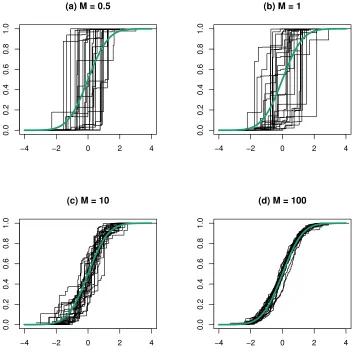
0 and variance 1. Figure 1.1 shows 25 draws from the DP G asαvaries from 0.5, 1, 10, and 100.
For eachα, the distribution function forG0over the interval[−4,4]is shown in bold. Whenα= 0.5,
few atoms contain the majority of the mass and the draws are clearly distinct (but centered around)
G0. This is true as well forα= 1, but the mass is more spread out across the atoms. Asα= 10,
draws from G are noticeably nearer toG0and whenα= 100, draws fromGare essentiallyG0. The
fact that the draws ofGare step functions demonstrates its discreteness.
The discreteness ofGhas its drawbacks, however. When dealing with continuous density
estima-tion, using a DP as the target distribution can be problematic. Instead, the DP is often used as a
Figure 1.1: Draws from a Dirichlet process.
−4 −2 0 2 4
0.0
0.2
0.4
0.6
0.8
1.0
(a) M = 0.5
−4 −2 0 2 4
0.0
0.2
0.4
0.6
0.8
1.0
(b) M = 1
−4 −2 0 2 4
0.0
0.2
0.4
0.6
0.8
1.0
(c) M = 10
−4 −2 0 2 4
0.0
0.2
0.4
0.6
0.8
1.0
(d) M = 100
Draws from a Dirichlet processG∼DP(G0, α)with base measureG0, which is normal with mean 0 and variance 1. The mass parameterαvaries between0.5and100. (a) 25 draws whenα= 0.5. The draws are distinct fromG0and consist mostly of a point that contains the majority of the mass. (b) 25 draws whenα= 1. Draws are still distinct fromG0but the mass is spread around to several points. (c) Draws withα= 10are starting to resembleG0. (d) Withα= 100, a draw fromGis nearly
G0itself.
yi|θi∼f(·;θi); (1.1)
θi|G∼G;
whereyiis a continuous random variable with densityfy(·)parameterized byθi. Here the density
of yi is given a known parametric form. Each observation has its own θi but having been drawn
from the discrete measureG, there is a positive probability of ties forθiamong observations. Thus,
some observations share the same θi. Integrating out the random probability measure yields an
infinite mixture of parametric distribution.
fG(y) =
Z
f(y;θ)dG(θ) (1.2)
=
∞
X
j=1
wjf(y; ˜θ), (1.3)
for some weightswj depending onG.
Contrast this to the parametric Bayesian model below:
yi|θ∼fy(·;θ); (1.4)
θ∼G0.
In the parametric version, the density is assumed to be of the formfy(·;θ). In the nonparametric
version with a DP mixture, the density is an infinite mixture offy(·;θ), which may assume arbitrary
shape. In this density estimation example, we achieve greater flexibility merely by placing a DP
prior in lieu of the parametric setup in which accuracy depends on correctly specifying the model
in equation (1.4). In the following section, we continue our examination of nonparametric Bayesian
priors focusing on function spaces.
Bayesian Additive Regression Trees
Consider an outcomeY and a vector of covariatesX. To estimateY givenX =x, we may assume
thatE(Y|X =x) =f(x)for some functionf(·). The functionf(·)can be parameterized byβ so
thatf(x;β) = xβ, as in linear regression (McCullagh, 1984). However, if we don’t want to make
the Bayesian paradigm, place a prior onf(·)itself. One such option is the Gaussian process prior
(Rasmussen, 2006). Note that we don’t have to place the probability model directly onf(·). Instead,
we can expandf(·)to be a sum of basis expansions (f(x) =Pβ
iφi(x)) and put priors on the basis
coefficients (M ¨uller et al., 2015). In the next chapter of this dissertation, we adhere to this latter
method using Bayesian Additive Regression Trees (BART) and write f(·)as a sum of Bayesian
regression trees (Chipman, George, and McCulloch, 2010).
BART is a machine learning algorithm used to estimate an unknown function and make predictions
of the outcome given covariates. To understand how BART works, it is necessary to understand
ter-minology and methodology for a single regression tree (Chipman, George, and McCulloch, 1998).
In the regression tree framework, the study population is split into subgroups based on a sequence
of rules. Within each subgroup subjects have a similar mean response. Trees consists of interior
nodes, splitting rules, and terminal nodes. Terminal nodes are the last node in a given sequence
of interior nodes and splitting rules at which point the outcomeY is summarized. An example of a
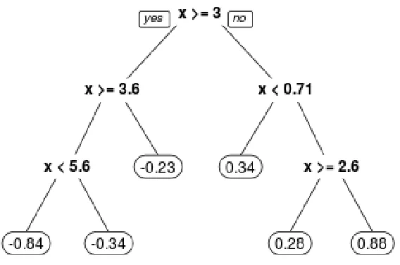
regression tree is shown in Figure 1.2. In this example, there is a single covariate predictive of a
countinuous outcome. A subject withx= 4would follow the leftmost path in the example figure, and
the mean outcome of all subjects following this path (i.e., with3.6≤x <5.6) is−0.84. Regression
trees are widely available in off-the-shelf statistical software. However, they yield non-smooth
esti-mates of the conditional distribution ofY givenX, which may not be desirable in some applications.
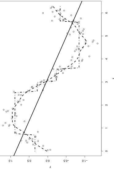
For an example of this, see Figure 1.3. We randomly choose points uniformly within the
univari-ate predictor spacex∈ [0,2π]. The outcomey is related toxthrough the relationy = sin(x) +
whereis a normal error term. We assume the relationship betweenyandxis unknown and that
the function relatingy toxis the target of inference. Since the functionsin(x)is non-linear, linear
regression is the incorrect approach (solid line). Using a regression tree (dotted-dashed line) is a
better fit than linear regression, but it still fails to capture the smoothness of the true function.
On the other hand, BART’s sum-of-trees structure is adept at capturing the smoothness (dashed
line in Figure 1.3). To implement BART, we setf(x) = P
ωi(x)whereωi(x)is a regression tree
and each ωi(x) is restricted to be small (few terminal nodes). The sum-of-trees is more flexible
and can better handle complex interactions and nonlinearities than a single tree. BART also has
relatively few tuning parameters, which makes it an attractive option when one doesn’t want to
generalized linear model setting where only a subset of the covariates are of scientific interest. The
nuisance component is modeled with BART and the covariates of interest are modeled
parametri-cally.
Figure 1.2: Example of a regression tree in a univariate covariate space.
Bayesian methods in causal inference
Literature involving Bayesian methods in causal inference has grown in recent years. These
in-clude implementations of marginal structural models (Roy, Lum, and Daniels, 2016; Saarela et al.,
2015) and the g-formula (Roy et al., 2017). In this dissertation, we aim to add to the literature by
developing nonparametric Bayesian methods with emphasis on causal methods. In Chapter 2, we
present a semiparametric regression model where only a small subset of covariates are of scientific
interest using BART to control for confounding from other covariates. We show how this model can
be used as a structural mean model, which has the advantage of avoiding g-estimation which is not
possible for the probit and logit link functions, two popular link functions with binary outcomes. In
Chapter 3, we present joint model for a continuous longitudinal outcome and the covariates using
an enriched Dirichlet process, an improvement of a standard DP when the dimension of covariates
is high. This offers improved prediction over competitor models and also serves as a functional
clustering algorithm. In Chapter 4, we use this joint model for causal inference using the parametric
Figure 1.3: Illustration of a BART fit with a univariate predictor space.
0
1
2
3
4
5
6
−1.0 −0.5
0.0 0.5
1.0
x
y
CHAPTER 2
B
AYESIAN SEMIPARAMETRIC REGRESSION AND STRUCTURAL MEAN MODELS WITHBART
Introduction
Semiparametric models, which include generalized estimating equations (GEE) and proportional
hazards models, are some of the most commonly used models in statistics (Tsiatis, 2006). While
the scope of semiparametrics is wide, the basic tenet is that we have a specific research
ques-tion that is of interest (e.g., the effect of a treatment on an outcome) but in order to answer that
question we must handle another part of the data that may not be of immediate scientific interest
(e.g., adjusting for confounders). This latter part is referred to as the nuisance. A fully parametric
model would need to model the nuisance parameters as well as the parameter of interest with a
parametric form, but a model can be semiparametric by leaving the part for the nuisance
param-eters unspecified. Ideally, the semiparametric model can answer the scientific question of interest
without inducing bias by the misspecification of the nuisance model.
The semiparametric framework is important in causal inference (Kennedy, 2016), which largely
avoids fully parametric models for the aforementioned reasons. One of the most popular causal
models, the marginal structural model, is semiparametric by leaving part of the conditional
dis-tribution of the outcome unspecified (Robins, Hernan, and Brumback, 2000). Marginal structural
models were developed for longitudinal settings to adjust for time-varying confounding. A related
but less used causal model, the structural mean model (SMM), is also semiparametric and was
also developed for scenarios with time-varying confounding (Robins, 1986; Robins, 1994). Both
marginal structural models and structural mean models can be used in the setting of an exposure
at a single time point and still parameterize a meaningful causal contrast (Robins, 2000). Solving for
the causal parameters in each of these models has been well documented in the literature (Hern ´an
and Robins, 2018; Hern ´an, Brumback, and Robins, 2000). In particular, solving for the parameters
of a SMM requires g-estimation, which amounts to solving estimating equations when the identity
or log link function is used, as is typical for continuous or count outcomes (Hern ´an and Robins,
easy solution exists for solving for the parameters of SMMs (Vansteelandt and Goetghebeur, 2003).
Methods for this case have been proposed but require specifying a second model, which may
in-troduce bias if specified incorrectly (Robins and Rotnitzky, 2004; Vansteelandt and Goetghebeur,
2003).
Recently, there have been Bayesian implementations of marginal structural models (Roy, Lum,
and Daniels, 2016; Saarela et al., 2015). However, no Bayesian implementation of SMMs exists,
though a fully parametric likelihood based model has been developed (Matsouaka and Tchetgen
Tchetgen, 2014). Our aim is to develop the first fully Bayesian SMM, yielding posterior distributions
for the causal parameters of interest while sidestepping the need for g-estimation and thus making
estimation more robust when the outcome is binary. In doing so, we also find that our method is
suitable for more general regression models, when causal assumptions might not be realistic or
of interest, and can be used as a robust and intuitive semiparametric regression model in place
of parametric regression. Our method can be easily implemented using our R packagesemibart,
which is available on the author’s website (https://www.github.com/zeldow/semibart).
The rest of the paper is organized as follows. Section 2 describes relevant background and a
literature review. In Section 3, we describe the types of semiparametric models we are fitting,
including SMMs and Bayesian semiparametric regression. Section 4 gives simulation results. In
Section 5 we complete a data analysis on the effect of initiating certain antiretroviral drugs on death
among adults with HIV infection who are newly initiating an antiretroviral regimen. In Section 6, we
discuss strengths and limitations of our method.
Background
Letybe an outcome and letXbe predictors ofy. Whenyis continuous, consider the regression
scenario yi = ω(xi) +i, with error terms assumed to be from from a distribution with mean
zero. For non-continuous outcomes, we consider the model E(y|X) = g(ω(X))for a given link
function g. The parametric linear regression which asserts thatω(xi;β) = P p
j=1βjxij with error termsi iid∼ N(0, σ2)is easily solved using Bayesian methods when prior distributions are placed
onβ and the regression error variance σ2(Gelman et al., 2014). For the remainder of this paper,
we focus on relaxing the assumption thatω(xi;β) =P p
j=1βjxij, which can yield biased estimates
Our approach in modeling the relationship between Y and X targets the conditional mean of Y
given X, which we denote asω(·). There is large statistical literature focused on modelingω(·)
flexibly; we review some of these with added emphasis on Bayesian methods. We can think ofω(·)
as a random function by placing a prior distribution on the function space. One possible prior is
the Gaussian process prior whose covariance structure can be specified such that the posterior
captures nonlinear structures (Rasmussen, 2006). Other options for modelingω(·)include the use
of basis functions (M ¨uller et al., 2015) like splines (Eilers and Marx, 1996) or wavelets and placing
prior distributions on the coefficients. Splines have been used extensively in Bayesian
nonpara-metric and semiparanonpara-metric regression. Biller (2000) presented a semiparanonpara-metric generalized linear
model where one variable is modeled using splines and the remaining variables were part of a
parametric linear model(Biller, 2000). Holmes and Mallick (2001) developed a flexible Bayesian
piecewise regression using linear splines (Holmes and Mallick, 2001). The approach in Denison
et al (1998) involved piecewise polynomials and was able to approximate nonlinearities (Denison,
Mallick, and Smith, 1998c). Biller and Fahrmeir (2001) introduced a varying-coefficient model with
B-splines with adaptive knot locations (Biller and Fahrmeir, 2001).
Two of the most commonly used semiparametric methods that predict an outcome Y given
co-variatesX are generalized additive models (GAM) (Hastie and Tibshirani, 1990) and multivariate
adaptive regression splines (MARS) (Friedman, 1991), both of which were developed as frequentist
procedures and are available in commonly used statistical software. GAM allows each predictor to
have its own functional form using splines. The downside of GAM is that any interactions between
covariates must be specified by the analyst, which can pose problems in high-dimensional problems
in which there may be many multi-way interactions. Bayesian versions of GAM based on P-splines
exist (Brezger and Lang, 2006) but do not have the widespread availability in statistical software
that the frequentist version has. MARS is a fully nonparametric procedure which can automatically
detect nonlinearities and interactions through basis functions also based on splines. A Bayesian
MARS algorithm has also been developed (Denison, Mallick, and Smith, 1998b) but also lacks
off-the-shelf software. A third option for nonparametric estimation ofY given X is Bayesian additive
regression trees (BART), which like MARS, is adept at capturing nonlinearities and interactions
between covariates, while being a fully Bayesian procedure (Chipman, George, and McCulloch,
Bayesian Additive Regression Trees
Bayesian additive regression trees (BART) is a machine learning algorithm designed to model an
outcome as a function of covariates and a normal, additive error term. LetY =ω(X) +whereY is
a continuous outcome,∼N(0, σ2), andω(·)is the unknown functional relating the predictorsX to
the outcomeY. For binaryY the probit link function is used, that is Pr(Y = 1|X) = Φ(ω(X)), where
Φ(·)is the distribution function of a standard normal random variable. While other link functions
for binary data (e.g., logit) are possible, using a probit link function simplifies Bayesian
compu-tations and is used in software implementing BART. BART estimates the function ω(·) through a
sum of regression trees, where a regression tree is a sequence of binary choices based on
predic-torsX which yield predictions of Y within clusters of observations with similar covariate patterns.
Classification and regression trees are typically frequentist procedures, but Bayesian versions of
regression trees have also been developed (Chipman, George, and McCulloch, 1998; Denison,
Mallick, and Smith, 1998a). The BART sum-of-trees model can be written asω(x) =Pm
i=1ωi(x),
where eachωi(x)is itself a tree. Typically, the number of treesmis chosen to be large and each
tree is restricted to have a small number of end nodes. This setup restricts the influence of any
single tree while allowing detection of nonlinearities and interactions that would be not possible
with one tree. An example of a BART fit to a nonlinear mean functiony = sin(x) + is shown in
Figure 1.3 over a univariate predictor spacexrestricted to[0,2π], along with comparision to the fit
of a single regression tree and linear regression.
The algorithm for BART utilizes Bayesian backfitting (Hastie, Tibshirani, et al., 2000). We review the
algorithm for the case of continuous outcomes; the case for binary outcomes is a simple extension
which utilizes the underlying normal latent variable formulation (Albert and Chib, 1993). Recall that
yi=Pm
j=1ωj(xi) +iwhereiis assumed zero-mean normal with unknown varianceσ
2. The
algo-rithm iterates between updating the error varianceσ2and updating the fit of the treesωj. The error
varianceσ2is updated by obtaining the residuals from the current fit and drawing the posterior from
an inverse chi-square distribution when the conjugate inverse-chi square prior is used. Second,
each treeωj is updated. For this step, we compute the residuals of the outcome by subtracting
off the fit of the otherm−1 trees. When updating tree ω1, the residualsy∗i = yi−
Pm
i=2ωj(xi) are calculated. The fit for ω1(·)is updated through a proposed change to the tree (grow, prune,
ω2(·), ω3(·), . . . , ωm(·)are all updated in the same fashion. More details are available in elsewhere
(Chipman, George, and McCulloch, 2010). In the next section, we propose a semiparametric
ex-tension of BART, which we call semi-BART, where a small subset of covariates are allowed to have
linear functional form and the rest are modeled with BART.
Semi-BART Model
Notation
Suppose we havenindependent observations. LetY denote the outcome, which we assume to be
either binary or continuous. Denote byLthe set of predictor variables. The outcome for individual
1≤i≤nwill be denoted asYi, with similar notation for covariatesLi.
Semiparametric Generalized Linear Model
Our model imposes linearity on just a small subset of covariates of interest, while remaining flexible
in modeling the rest of the covariates, whose exact functional form in relation to the outcome may be
considered a nuisance. The predictors are partitioned into two distinct subsets so thatL=L1∪L2
andL1∩L2 = ∅. Here, L1 represents nuisance covariates that we must control for but is not of
primary interest andL2represents covariates that do have scientific interest. For continuousY, we
writeYi =ω(L1) +h(L2;ψ) +i, whereh(·)is a linear function of its covariates inψ(as in linear
regression) butω(·)is a function with unspecified form. The errorsiare iid mean zero and normally
distributed with unknown varianceσ2. More generally, we writeg[E(Y|L
1,L2)] = ω(L1) +h(L2),
for a given link functiong. We estimateω(·)using BART. Note that this implies that ifL1=Land
L2 =∅, we have a nonparametric BART model. On the other hand ifL1=∅andL2=L,we have
a fully parametric regression model. While there is no restriction on the dimensionality ofL1and
L2, in the typical caseL1is large enough that BART is a reasonable choice of an algorithm andL2
contains only a few covariates that are of particular interest.
Special Case: Structural Mean Models
We now consider the special case of a causal inference setting with observational data. We
in-troduce further notation specific to this section. The exposure of interest is denoted A and can
observed under exposureA=a. For the special case of binaryA, each individual has two
coun-terfactual outcomes – Y1and Y0 – but we observe at most one of the two, corresponding to the
actual level of exposure received. That is,Y =AY1+ (1−A)Y0.LetXbe the set of confounders.
We can further subsetXintoX = (X1,X2), whereX2 is the subset of variables that modify the
causal effect ofAandX1 are the other covariates. From the notation in the previous subsection,
we can then think ofL2= (A,X2)as the variables of primary interest andL1=X1as the variables
that are not of interest but need to be controlled for.
Structural nested mean models are causal models developed by Robins to deal with time-varying
confounding for longitudinal exposures (Robins, 1994, 2000). In the case of point treatment,
struc-tural nested mean models are referred to as strucstruc-tural mean models (SMMs) and parameterize a
useful causal contrast even though time-varying confounding is not a concern (Vansteelandt and
Joffe, 2014; Vansteelandt and Goetghebeur, 2003). This contrast encodes the mean effect of
treat-ment among the treated given the covariates. The model can generally be written as:
g{E(Ya|X=x, A=a)} −g
E Y0|X=x, A=a =h∗(x, a;ψ∗), (2.1)
whereg is a known link function. Here we switch fromh(·;ψ)to h∗(·;ψ∗)to indicate thatψ∗ rep-resents a causal effect, but the two functions and parameters are otherwise identical. The goal of
this paper is to provide a Bayesian solution to (2.1). First, we impose some restrictions onh(·;ψ∗). We require that under no treatment or when there is no treatment effect the functionh∗(·;ψ∗)must equal 0. That is,h∗(x, a;ψ∗)satisfiesh∗(x, a; 0) =h∗(x,0;ψ∗) = 0. Some examples ofh∗(·;ψ∗)are
h∗(x, a;ψ∗) =ψaorh∗(x, a;ψ∗) = (ψ1+ψ2x)a, whenxis thought to be an effect modifier.
While expression (2.1) cannot be evaluated directly because of the unobserved counterfactuals,
two assumptions are needed to identify it with observed data (Vansteelandt and Joffe, 2014).
1. Consistency: IfA=a, thenYa=Y;
2. Ignorability: A⊥Y0|X.
The consistency assumption says that we actually get to see an individual’s counterfactual
corre-sponding to the exposure received. Ignorability ensures that there is no unmeasured confounding
assump-tions together with the parametric assumption ofh∗(·), the contrast on the left hand side of (2.1) is identified, and the SMM from (2.1) can be rewritten using observed variables as
g{E(Y|X, A)}=ω(L2) +h∗(L1;ψ∗), (2.2) where ω(L1) is unspecified and h∗(L2;ψ∗) is a linear function of X2 and A (Vansteelandt and Joffe, 2014). While we use the above assumptions for the remainder of this paper, the left hand
side of (2.1) can be nonparametrically identified with a third assumption, dropping the parametric
assumption ofh∗(·). That is,
3. Positivity: Pr(A=a|X=x)>0∀xsuch that Pr(X=x)>0.
The positivity assumption states that within all covariate levelsX=xthat have positive probability
of occurring, there is positive probability that an individual is treated. This assumption is violated in
situations where treatment is deterministic at specific levels ofX=x.
It should be noted that we have chosen a parametric form for all ofX2, including the main effects
of effect modifiers. In principal, one could includeX2in the nonparametric part and only model the
interactionX2×Aparametrically. For example, if a researcher posits the relationshiph∗(x, a;ψ∗) = (ψ1+ψ2x)a, the variable xin principle could be modeled nonparametrically. In simulations, we
have found that including the covariatesX2into the BART model as well generally leads to poorer
performance (bias, under coverage) of the causal effect posterior distributions. As a result, we
would opt for the linear modelh∗(x, a;ψ∗) = (ψ1+ψ2x)a+ψ3xin our example. Further, in practice if researchers are interested in effect modification byX2they might also be interested in interpreting
the main effect.
Hill, 2011 has previously modeled causal effects on the treated using BART. The methods
de-scribed in that paper correspond to our setting in equation (2.2) wheregis the identity link function
andψ∗ is a scalar describing only an effect of treatment with no effect modification. Our method extends this setup to settings with binary outcomes, continuous-valued treatment, or where
low-dimensional summaries of effect modification are of interest. In settings with continuous outcomes,
binary treatment, and no effect modification, the methods presented in Hill, 2011 may be preferred.
Computations
The algorithm for semi-BART follows the BART algorithm with an additional step. We briefly
re-viewed the algorithm in Section 2.2.1. Below, we describe the basics of our algorithm for
semi-BART. We are solving equation (2.2), whereω(L2)can be written as the sum-of-treesP
m
j=1ωj(L2). Each treeωj(L2)has a vector of parametersθj associated with it. The mean of thekthendnode of
thejthtree is assumed to be normally distributed with meanµjkand varianceσ2
jk.
Recall that when the outcome is continuous, we assume independent errors distributedN(0, σ2).
The algorithm for semi-BART for continuous outcomes is as follows. First, we initialize all values
including the error varianceσ2, the parametersψ∗, and the tree structureω(L1)for allmtrees. Next we begin our MCMC algorithm and iterate through the following steps. First update themtrees one
at a time. When updating thejthtree, subtract the fit of the remainingm−1trees at their current
parameter values as well as the fit of the linear parth∗(L2;ψ∗)at the current value ofψ∗ from the value ofyfor each individual. That is, we calculateyi∗=yi−ω−j(L1i)−h∗(L2i;ψ∗), whereω−j(L1i)
indicates the fit of them−1without thejthtree. A modification of thejthtree is now proposed. We
either grow the tree (add a split point to what was previously an endnode), prune the tree (collapse
two endnodes into one), change a splitting rule (for nonterminal nodes), or swap the rules between
two nodes. Once a modification is proposed, we accept or reject this modification with a
Metropolis-Hastings step (Chipman, George, and McCulloch, 1998). The parametersθjare then updated from
draws based on the conjugate priors (normal priors forµjkand inverse chi-squared forσ2jk).
Next we update ψ∗. To do this, we calculate the residuals after subtracting off the fit of all m
trees. That is, calculate y∗i = yi−ω(L1i). With a conjugate multivariate normal prior with mean
ψ0 and varianceσ2ψIonψ
∗ whereIis the identity matrix of appropriate dimension, updatingψ∗is
simply a draw from a multivariate normal distribution. The posterior forψis multivariate normal with
covarianceΣψ=
hLT 2L2
σ2 +
I
σ2 ψ
i−1
and meanΣψ
hL
2y∗
σ2 +
ψ0
σ2 ψ
i
(Gelman et al., 2014).
Finally, we update σ2. We calculate the residuals by conditioning on the fitted trees θi and the
parametric part ψ∗ and subtracting off the fit of all m trees and the linear part h∗(·). That is, calculatey∗i =yi−ω(L1i)−h(L2i;ψ∗). We use a conjugate inverse chi squared distribution forσ2
and draw from an updated inverse chi squared distribution. We then return to updating each of the
The algorithm for binary outcomes with a probit link uses the underlying latent continuous variable
formulation of (Albert and Chib, 1993) and is inserted into the algorithm in lieu of updating the
error variance σ2. Further details of the latent variable step as well as other steps pertaining to
BART such as choosing a variable for a split point or choosing the splitting rule can be found in
(Chipman, George, and McCulloch, 2010). The full implementation of our algorithm is available at
https://www.github.com/zeldow/semibart.
Simulations
We used simulation to assess performance of our model under both continuous and binary
out-comes. We generated five binary covariates (x1, . . . , x5) from independent Bernoulli random
vari-ables and twenty continuous covariates (x6, . . . , x25) from a multivariate normal distribution for a
total of 25 predictors. The binary covariatex1is considered to be the treatment variable. The
co-variatesx6, . . . , x10 were generated with non-zero correlation with each other but independent of
the rest, as were covariatesx11, . . . , x15, covariatesx16, . . . , x20, and covariatesx21, . . . , x25. Exact
distributions for covariate generation are given in the Appendix (Section A). Outcomes were
gener-ated with both linear and non-linear mean functions and were relgener-ated to only the first 10 covariates.
In the continuous case, outcomes were generated from a normal distribution with standard
devia-tions 0.1, 1, 2, and 3 (results in the main text are presented with a standard deviation of 1). In the
linear cases, outcomes were given meanµ`,1= 1+2x1+2x5+2x6−0.5x7−0.5x8−1.5x10when only
the effect ofx1was of interest, orµ`,2= 1 + 2x1+ 2x5+ 2x6−0.5x7−0.5x8−1.5x10−x1x6when
effect modification of x6 onx1 was also of interest. For nonlinear models, outcomes were given
meanµnl,1= 1 + 2x1+ 2x6+ sin(πx2x7)−2 exp(x3x5) + log |cos(π2x8)|
−1.8 cosx9+ 3x3|x7|1.5or
µnl,2= 1 + 2x1+ 2x6+ sin(πx2x7)−2 exp(x3x5) + log |cos(π2x8)|
−1.8 cosx9+ 3x3|x7|1.5−x1x6, for
no effect modification and effect modification, respectively. Our goal was to predict the treatment
effect ofx1and when appropriate, the effect modification of x6 onx1. For the linear case, linear
regression is the correctly specified model. In the non-linear cases, the treatment effect and the
effect modification are linear but the rest of the covariates have a nonlinear relationship with the
outcome. In addition to comparing semi-BART and linear regression, we also estimated effects
with doubly robust g-estimation with logistic regression for the treatment model and linear
regres-sion for the outcome model. Since the treatment is generated independently, the treatment model
the treatment effect using Hill’s estimate of the treatment effect on the treated using BART (Hill,
2011).
For binary outcomes, we generated 25 covariates in the same way, but outcomes were generated
from a Bernoulli distribution. For the linear case with no effect modification, outcomes were
gener-ated with probabilityp`,1= Φ(0.1+0.3x1+0.1x2+0.04x6−0.02x7+0.04x9−0.03x10), whereΦ(·)is the
distribution function for a standard normal variable. For the linear case with effect modification (of
x6onx1), outcomes were generated with probabilityp`,2= Φ(0.1 + 0.3x1+ 0.1x2+ 0.04x6−0.02x7+
0.04x9−0.03x10−0.1x1x6). In the nonlinear case, outcomes were generated with probabilitypnl,1=
Φ(0.1 + 0.3x1+ 0.04x6−sin(πx2x7) +101 exp(x7/3) +1[x9>2]cos(x8) +1[x9<1]cos(x10)−0.01x7x8x10)
when there was no effect modification andpnl,2= Φ(0.1+0.3x1+0.04x6−sin(πx2x7)+101 exp(x7/3)+
1x9>2cos(x8) +1x9<1cos(x10)−0.01x7x8x10−0.1x1x6)with effect modification betweenx6andx1.
Again, we are interested in extracting the treatment effect ofx1on the outcome, and if applicable,
the effect modification ofx6onx1. We estimate these effects from semi-BART and probit
regres-sion and compare results from the two models. For the linear case, probit regresregres-sion is the correctly
specified model.
For all scenarios, we generated 500 datasets each at sample sizes ofn= 250,1000,and5000. All
models are compared on mean bias, 95% coverage probability of the confidence or credible interval,
and mean squared error (MSE). For semi-BART, we used 10,000 total iterations the first 2,500 of
which were burn-in. For the BART part of the model we used 200 trees. The prior distribution on
the parameters of interest was independent mean zero normal with a standard deviation of 4, which
is a diffuse prior given that the outcome was scaled and centered to be between −1 2 and
1 2. For
Hill’s treatment on the treated with BART, we used all default values from the BayesTree package
in R (Chipman, George, and McCulloch, 2010).
Continuous Outcome - No Effect Modification
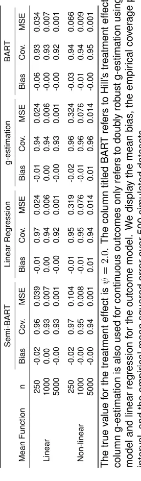
The results of our simulations for continuous outcomes with no effect modification is shown in
Table 2.1. Outcomes were generated with a standard deviation of 1. The true parameter for the
treatment effect isψ= 2.0. In the linear case (shown in the top half of the table and generated by
mean functionµ`,1), linear regression is the correctly specified model. As expected, it has lower
semi-BART and the pure semi-BART results are unbiased and are nearly as efficient as linear regression at
n= 5000(MSE = 0.001 for all). G-estimation, being comprised of linear models as well, is nearly
equivalent to linear regression in terms of bias, coverage, and MSE. The lower half of Table 2.1
shows the results when the mean function is largely non-linear, generated through mean function
µnl,1. In this scenario, semi-BART and BART have much lower MSE than linear regression at all
sample sizes. All methods are unbiased with good coverage. Note that at n = 250, the MSE
for BART is 0.066 while the MSE for semi-BART is 0.104. Results for these simulations using
outcomes drawn with standard deviations 0.1, 2, and 3 are displayed in Appendix B, Tables B.1,
B.2, and B.3, respectively. The results are similar to those in Table 2.1.
Continuous Outcome - Effect Modification
The results of our simulations with a continuous outcome and a continuous effect modifier for the
treatment effect are shown in Table 2.2. The true value for the treatment effect isψ1 = 2.0 and
the true value for the effect modification ofx6 on the treatment isψ2 =−1.0. In the top half of the
table denoting the linear case generated by mean function µ`,2, linear regression is the correctly
specified model. Atn = 250, linear regression has lower MSE forψ1 than semi-BART (0.126 vs.
0.153) and for ψ2 (0.025, 0.031). At n = 5000, the two methods have the same rounded MSE
(0.005 forψ1and 0.001 forψ2). All methods are unbiased with coverage around the nominal level.
In the non-linear case (generated by mean functionµnl,2, the bias forψ1 using linear regression is
slightly larger in absolute value than for semi-BART or g-estimation (-0.07 for linear regression and
-0.03 for the rest). In terms of MSE, semi-BART is much more efficient than linear regression for
both parameters and all sample sizes compared to linear regression and g-estimation with linear
models. Results for these simulations using outcomes drawn with standard deviations 0.1, 2, and 3
are displayed in Appendix B, Tables B.4, B.5, and B.6, respectively. The results are similar to those
in Table 2.2.
Binary Outcome - No Effect Modification
The simulation results with a binary outcome and no effect modification are shown in Table 2.3.
The true value for the treatment effect isψ= 0.3. In the linear case, outcomes are generated with
probabilityp`,1 and probit regression is the correctly specified model. In the non-linear case with
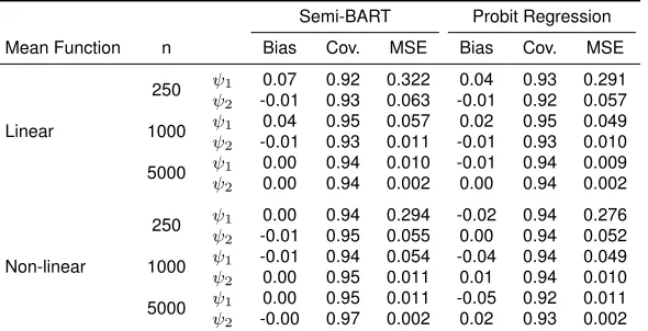
Table 2.2: Efficiency of Semi-BART for a continuous outcome with effect modification.
Semi-BART Linear Regression g-estimation
Mean Function n Bias Cov. MSE Bias Cov. MSE Bias Cov. MSE
Linear
250 ψ1 -0.01 0.96 0.153 0.02 0.96 0.126 0.01 0.93 0.141 ψ2 0.00 0.96 0.031 -0.01 0.95 0.025 -0.00 0.93 0.029
1000 ψ1 -0.00 0.96 0.029 -0.00 0.96 0.027 0.00 0.95 0.027 ψ2 0.00 0.97 0.006 0.00 0.96 0.005 0.00 0.95 0.005
5000 ψ1 0.01 0.95 0.005 0.00 0.96 0.005 0.00 0.96 0.005 ψ2 -0.00 0.96 0.001 -0.00 0.95 0.001 -0.00 0.96 0.001
Non-linear
250 ψ1 -0.03 0.98 0.450 -0.07 0.94 1.570 -0.03 0.94 1.991 ψ2 0.01 0.96 0.102 0.03 0.94 0.332 0.01 0.92 0.432
1000 ψ1 -0.00 0.95 0.039 -0.01 0.94 0.332 -0.01 0.96 0.362 ψ2 0.01 0.94 0.008 0.01 0.94 0.073 0.00 0.96 0.082
5000 ψ1 -0.00 0.95 0.006 0.01 0.96 0.068 0.02 0.96 0.075 ψ2 0.00 0.95 0.001 -0.00 0.94 0.015 -0.01 0.96 0.017
The true value for the treatment effect isψ1= 2.0and the true value pertaining to effect modification betweenx1andx6 isψ2 =−1.0. The column g-estimation is also used for continuous outcomes only refers to doubly robust g-estimation using logistic regression for the treatment model and linear regression for the outcome model
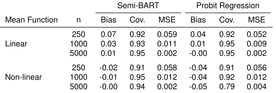
Table 2.3: Efficiency of Semi-BART for a binary outcome without effect modification.
Semi-BART Probit Regression
Mean Function n Bias Cov. MSE Bias Cov. MSE
Linear
250 0.07 0.92 0.059 0.04 0.92 0.052
1000 0.03 0.93 0.011 0.01 0.95 0.009 5000 0.01 0.95 0.002 -0.00 0.95 0.002
Non-linear
250 -0.02 0.91 0.058 -0.04 0.91 0.056 1000 -0.01 0.95 0.012 -0.04 0.92 0.012 5000 -0.00 0.94 0.002 -0.05 0.79 0.004
The true value for the treatment effect isψ= 0.3.
for semi-BART and 0.04 for probit regression). The bias gets smaller for both models as the sample
size increases. The MSE for probit regression is smaller than semi-BART at all sample sizes, but
the difference is not as pronounced as with continuous outcomes in Table 2.1. In the non-linear
case with outcomes generated with probability,pnl,1, there is slight initial bias for semi-BART (-0.02)
and probit regression (-0.04). However, the bias for probit regression is persistent at all sample
sizes whereas the bias vanishes in the semi-BART model. In terms of MSE, semi-BART and probit
regression are similar, except perhaps atn= 5000where the MSE with semi-BART is 0.002 versus
Table 2.4: Efficiency of Semi-BART for a binary outcome with effect modification.
Semi-BART Probit Regression
Mean Function n Bias Cov. MSE Bias Cov. MSE
Linear
250 ψ1 0.07 0.92 0.322 0.04 0.93 0.291 ψ2 -0.01 0.93 0.063 -0.01 0.92 0.057
1000 ψ1 0.04 0.95 0.057 0.02 0.95 0.049 ψ2 -0.01 0.93 0.011 -0.01 0.93 0.010
5000 ψ1 0.00 0.94 0.010 -0.01 0.94 0.009 ψ2 0.00 0.94 0.002 0.00 0.94 0.002
Non-linear
250 ψ1 0.00 0.94 0.294 -0.02 0.94 0.276 ψ2 -0.01 0.95 0.055 0.00 0.94 0.052
1000 ψ1 -0.01 0.94 0.054 -0.04 0.94 0.049 ψ2 0.00 0.95 0.011 0.01 0.94 0.010
5000 ψ1 0.00 0.95 0.011 -0.05 0.92 0.011 ψ2 -0.00 0.97 0.002 0.02 0.93 0.002
The true value for the treatment effect is ψ1 = 0.3 and the true value for the effect modification parameter isψ2=−0.1.
Binary Outcome - Effect Modification
Results for a binary outcome with a continuous effect modifier for the treatment effect are shown
in Table 2.4. The true value for the treatment effect is ψ1 = 0.3 and the true value for the effect
modification parameter isψ2=−0.1. In the linear case, outcomes were generated with probability
p`,2. Here, probit regression is more efficient than semi-BART at low sample sizes (the MSE for
both parameters is about 1.1 times higher at n = 250). There is some bias atn = 250, that of
semi-BART is higher than that of probit regression (0.07 verus 0.04 forψ1). However, atn= 5000,
the results from the two models are nearly identical, as the bias in semi-BART went to 0. For the
non-linear case, outcomes were generated with probability pnl,2. Here, probit regression shows
some persistent bias forψ1, which is not the case for semi-BART. Despite this, the MSEs for probit
regression and semi-BART are nearly identical, driven by the lower empirical variance of estimates
from probit regression.
Data Application
To illustrate our method we analyzed data from the Veterans Aging Cohort Study (VACS) from
2002 to 2009, which is a cohort of HIV-infected patients being treated at Veterans Affairs facilities
in the United States. Our study sample consisted of patients with HIV/Hepatitis C coinfection who
were newly initiating antiretrovirals (including at least one nucleoside reverse transcriptase inhibitor
NRTIs are known to cause mitochrondial toxicity. These mitochrondial toxic NRTIs (mtNRTIs)
in-clude didanosine, stavudine, zidovudine, and zalcitabine (Soriano et al., 2008). While these drugs
are no longer part of first line HIV treatment regimens, they are still used in resource-limited settings
or in salvage regimens (G ¨unthard et al., 2016).
Exposure to mtNRTIs may increase the risk of hepatic injury which in turn may increase the risk
of hepatic decompensation and death (Scourfield et al., 2011). The goal of this analysis was to
determine if initiating an antiretroviral regimen containing a mtNRTI increased the risk of death
ver-sus antiretroviral containing a NRTI that is not a mtNRI. VACS data contains a number of variables
confounding the relationship between mtNRTI use and death including subject demographics, year
of antiretroviral initiation, HIV characteristics such as CD4 count and HIV viral load, concomitant
medications, and laboratory measures relating to liver function.
One of the covariates included in our analysis is Fibrosis-4 (FIB-4), an index that measures hepatitic
fibrosis with higher values indicating larger injury. Specifically FIB-4 > 3.25 (no units) indicates
advanced hepatic fibrosis. FIB-4 can be calculated as:
[age (years)×AST (U/L)]/hplatelet count(109/L)×pALT (U/L)i
(Sterling et al., 2006). Here, AST stands for aspartate aminotransferase and ALT for alanine
amino-transferase. There is some concern in that mtNRTI use in subjects with high FIB-4 will result in
higher risk of liver decompensation and death than in subjects who have low FIB-4. Thus, we
consider FIB-4 as a possible effect modifier of the effect of mtNRTIs on death.
The outcome is a binary indicator of death within a two-year period after the subject initiated
an-tiretroviral therapy. While covariates were updated in the study, we only considered baseline values
for this analysis. There were some missing values among the predictors that were handled through
a single imputation. A previous analysis of this data used multiple imputation to handle missing
covariates but found that results were very similar across imputations. All continuous covariates
were centered at meaningful values. For example, age was centered around 50 years and year of
study entry was centered at 2005.
effect modification, and to this extent we fit a Bayesian SMM with a probit link. The estimand can
be written as
Φ−1{E(Ya|X=x, A=a)} −Φ−1
E Y0|X=x, A=a =ψa, (2.3)
whereY is the indicator of death, A represents whether mtNRTIs were part of the antiretroviral
regimen at baseline (A = 1if mtNRTI were included in the regimen), andXall other covariates,
including FIB-4. In the second and third analysis, we considered FIB-4 to be an effect modifier,
once as a continuous covariate and once as a binary indicator which equaled 1 whenever FIB-4
>3.25. This estimand can be written as
Φ−1{E(Ya|X=x, A=a)} −Φ−1
E Y0|X=x, A=a =ψ1a+ψ2ax1, (2.4)
wherex1corresponds to the appropriate FIB-4 variable.
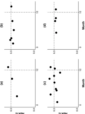
The analysis was conducted usingm= 200trees with 20,000 total iterations (5,000 burn-in). The
prior distribution on the ψ parameters were independent Normal(0,42). In the first analysis the
mean estimate of the posterior distribution forψwas 0.15 (95% credible interval (CI): -0.02, 0.33).
Notably the interval includes 0, but the direction of the point estimate indicates that subjects initiating
antiretroviral therapy with an mtNRTI had greater risk of death within 2 years than subjects initiating
therapy without an mtNRTI. We can interpret this coefficient in terms ofE Y0|X=x, A=aand
E(Ya|X=x, A=a)through the causal contrast in equation (2.3). Figure 2.1a shows the value of
E(Y1|X=x, A= 1)as a function ofE(Y0|X=x, A= 1)forψ= 0.15. As an example, suppose the
unknowable quantityE(Y0|X=x, A= 1) = 0.20. This means that subjects treated with a mtNRTI
(A= 1) with covariatesX=xwould have had a probability of death of20%within 2 years had they
been untreated (A= 0). However, givenψ = 0.15we see that ifE(Y0|X=x, A= 1) = 0.20then
E(Y1|X =x, A = 1) = 0.24, an increase of 4%. One can examine the change in probability for
other base probabilitiesE(Y0|X=x, A= 1)by examining the graph in Figure 2.1a. The trace plot
for this analysis is given as Figure A.1 in Section A.3 of the Appendix.
We conducted a second analysis with FIB-4 as a continuous effect modifier (centered around 3.25)
with the same settings as the previous one. This analysis corresponds to the contrast from
interaction between mtNRTI use and FIB-4 wasψ2= 0.07(0.02, 0.12). The results can be viewed
in Figure 2.1b. Again, for illustration, consider the special case whereE(Y0|X=x, A= 1) = 0.20.
When FIB-4 is 3.25, thenE(Y1|X=x, A= 1) = 0.25. However, at larger values such as a FIB-4
of 5.25, E(Y1|X = x, A = 1) = 0.30. The trace plot for this analysis is given as Figure A.2 in
Section A.3 of the Appendix.
Finally we did a third analysis with FIB-4 as a binary effect modifier (> 3.25vs. ≤ 3.25). Here
we found thatψ1 = 0.07(-0.12, 0.26) andψ2= 0.38(0.07, 0.69). These results can be viewed in
Figure 2.1c. Here, we see that ifE(Y0|X =x, A = 1) = 0.20, thenE(Y1|X =x, A = 1) = 0.22
for subjects with FIB-4≤3.25andE(Y1|X=x, A= 1) = 0.35for subjects with FIB-4>3.25. The
trace plot for this analysis is given as Figure A.3 in Section A.3 of the Appendix.
Discussion
We presented a new Bayesian semiparametric model, which can be implemented with an R
pack-agesemibartthat is available from the author’s GitHub page (https://github.com/zeldow/semibart).
Our model allows for flexible estimation of the nuisance parameters while being fully parametric
for covariates that are of immediate scientific interest, providing a viable and intuitive alternative to
fully parametric regression. Under some causal assumptions, this model can as be interpreted as
a SMM, which also provides the first fully Bayesian SMM. This is particularly useful in the case of
binary outcomes where g-estimation is not possible. Vansteelandt (2003) provided approaches for
estimating SMMs with binary outcomes in frequentist settings; our method is consistent with their
suggestions but incorporates the added flexibility of BART (Vansteelandt and Goetghebeur, 2003) .
In simulations we showed that semi-BART performs nearly as well as probit and linear regression
when the probit or linear model is correctly specified. On the other hand, when there is nonlinearity
in the mean functions or many interactions between covariates, using semi-BART provided
consid-erable benefits in our simulations in terms of efficiency (lower MSE for continuous outcomes) or bias
(lower bias for binary outcomes). G-estimation is possible for SMMs with continuous outcomes. In
our simulations with continuous outcomes, we used doubly robust g-estimation with linear models
for both the treatment and the response, which we chose for simplicity and because the model for
the treatment was correctly specified which would provide unbiased estimators. In practice, it may
the true data generating distribution. Another method we examined was Hill’s treatment effect on
the treated which we used in simulations with continuous outcomes and no effect modifier for
treat-ment (Hill, 2011). In this scenario, using Hill’s method is preferable because all covariates including
treatment can be modeled together using BART, whereas the semi-BART model utilizes the
treat-ment variable in a separate step from the other covariates. However, the modeling advantage of
semi-BART is that it provides a useful alternative to other Bayesian models when low-dimensional
summaries of effect modification are of interest. Furthermore, when in the settings of SMMs with
binary outcome, semi-BART is an alternative to other models, as g-estimation is not possible.
Some limitations of semi-BART are that it currently does not accommodate instrumental variables or
longitudinal treatment measures. Furthermore, its Bayesian implementation makes handling issues
such as censoring bias using inverse probability weights difficult (Robins, Hern ´an, and Wasserman,
2015). As seen in simulations, semi-BART performs best at higher sample sizes, though we found
reasonable results atn= 250with 25 covariates. Semi-BART is currently being extended to handle
Figure 2.1: Effect of mtNRTIs on death using semi-BART on cohort of individuals with HIV-HCV coinfection newly initiating HAART.
0.0 0.1 0.2 0.3 0.4 0.5
0.0 0.1 0.2 0.3 0.4 0.5 (a)
E(Y0| X, A=1)
E(
Y
1
| X, A=1) (0.20, 0.24)
0.0 0.1 0.2 0.3 0.4 0.5
0.0 0.1 0.2 0.3 0.4 0.5 (b)
E(Y0| X, A=1)
E(
Y
1
| X, A=1) (0.20, 0.25)
(0.20, 0.30)
FIB−4 = 3.25 FIB−4 = 4.25 FIB−4 = 5.25
0.0 0.1 0.2 0.3 0.4 0.5
0.0 0.1 0.2 0.3 0.4 0.5 (c)
E(Y0| X, A=1)
E(
Y
1
| X, A=1)
(0.20, 0.22) (0.20, 0.35)
FIB−4 <= 3.25 FIB−4 > 3.25
Results of data application using semi-BART on cohort of individuals with HIV-HCV coinfection newly initiating HAART. A = 1 indicates receipt of HAART with a mtNRTI andA = 0 indicates receipt of HAART without a mtNRTI. The x-axis shows possible mean values forE(Y0|X, A = 1)
which indicates the mean probability of death if the treatedA= 1had in fact been untreatedA= 0
given X. This quantity is unknown so we consider a spectrum of reasonable values. The y-axis
E(Y1|X, A = 1) gives the effect of treatment A on the quantity given by the x-axis. No causal effect of A would be indicated by a line with slope 1 through the origin. (a) In this analysis, we only consider that effect of mtNRTI (A) on death (Y) with no effect modifiers. The figure shows that ifE(Y0|X, A = 1) = 0.20thenE(Y1|X, A = 1) = 0.24, providing evidence that treatmentA is harmful. The magnitude of the causal effect of A onY is determine in part by the assumed value ofE(Y0|X, A= 1).(b) We consider the effect modification of mtNRTI on death by continuous FIB-4. The solid line indicates the causal effect curve when FIB-4 = 3.25 (the value we center FIB-4 around). At this value, assuming the base probability of death is 20%, that isE(Y0|X =x, A =
1) = 0.20, we find that treatment increases this risk to 25%. However, the mean risk of death for