EOQ Model for both Ameliorating and Deteriorating Items with
Exponentially Increasing Demand and Linear Time Dependent
Holding Cost
Yusuf I. GwandaTahaa Amin Ashiru Bala Bichi Muhammad Ado Lawan Deparment of Mathematics,
Kano University of Science and Technology-Wudil Abstract
An economic ordering quantity model for items that are both ameliorating and deteriorating with exponentially increasing demand and linear time dependent holding cost was developed. 1. Introduction
Demand for inventory items may sometimes sour high or nose dive suddenly or remain steady as dictated by the vicissitudes of life. A lot of inventory models were developed to explain such scenarios. The first model describing an exponentially decreasing demand for an inventory item was proposed by Hollier and Mak (1983) were they obtained optimal replenishment policies under both constant and variable replenishment intervals. Hariga and Bankerouf (1994) generalized Hollier and Mak (1983)’s model by taking into account both exponentially growing and decaying markets. Wee (1995, 1995) proposed a deterministic lot size model for deteriorating items where demand declines exponentially over a fixed time horizon. Later, Mishra et al (2013) studied an inventory model with non-instantaneous receipt and the exponential demand rate under trade credits. The paper determines optimal replenishment policies under conditions of non-instantaneous receipt and trade credits for two
optimal cycle time, optimal receipt period and total relevant cost. An inventory model for deteriorating items with exponential declining demand and time varying holding cost was studied by Dash et al. (2014).
The logarithmic demand for inventory models was studied by Pande et al. (2012). The study was an attempt to propose an inventory control model for fixed deterioration and logarithmic demand rate for the optimal stock of commodities to meet the future demand which may either arise at a constant rate or may vary with time. The analytical development is provided to obtain the optimal solution to minimize the total cost per time unit of an inventory control system. Numerical analysis has been presented to accredit the validity of the mentioned model. Effect of change in the values of different parameters on the decision variable and objectives function has been studied.
Singh et al. (2011) studied a Production Model with Selling Price Dependent Demand and Partial Backlogging under Inflation. Deterioration rate is taken as two parameter Weibull distribution. Shortages are allowed with backlogging and the backlogging rate is taken as exponential decreasing function of time.
Khanra et al. (2011) studied an EOQ Model for a Deteriorating Item with Time Dependent Quadratic Demand under Permissible Delay in Payment. Khanra et al. (2011) analyzed an EOQ model for deteriorating item considering time-dependent quadratic demand rate and permissible delay in payment. Among the various time-varying demand in EOQ models, the more realistic demand approach is to consider a quadratic time dependent demand rate because it represents both accelerated and retarded growth in demand. They therefore developed their mathematical models under two different circumstances:
Case II: The credit period is greater than the cycle time for settling the account.
Chung and Tsai (2001) studied an Inventory Systems for Deteriorating Items with Shortages and a Linear Trend in Demand-Taking Account of Time Value of money. They used a simple solution algorithm with a line search to obtain the optimal interval.
Mishra and Mishra (2008) studied Price determination for an EOQ model for deteriorating items under perfect competition. They used the concept of perfect competition as an important market structure. Under its effect, the price of a unit item of the EOQ model has been analyzed and computed by employing the approach of marginal revenue and marginal cost along with the profit optimization technique.
Moncer (1997) studied optimal inventory policies for perishable items with time-dependent demand. Moncer (1996) presents two computationally efficient solution methods that determine the optimal replenishment schedules for exponentially deteriorating items and perishable products with fixed lifetime. For both models, the inventoried items have general continuous-time-dependent demand.
Deepa and Khimya (2013) studied the stochastic inventory model for ameliorating items under supplier’s trade credit policy. Spectral theories are used to derive explicit expression for the transition probabilities of a four state continuous time markov chain representing the status of the systems. These probabilities are used to compute the exact form of the average cost expression. They used concepts from renewal reward processes to develop average cost objective function. Optimal solution is obtained using Newton Raphson method in R programming.
ameliorating items. Obtaining an instantaneous replenishment model for such items under cost minimization.
Valliathal (2013) studied an inflation effects on an EOQ model for weibull deteriorating/ameliorating items with ramp type of demand and shortages. Valliathal (2013) studied the replenishment policy, starting with shortages under two different types of backlogging rates, and their comparative study was also provided. He then used the computer software, MATLAB to find the optimal replenishment policies and obtain the inflation effects. Barik et al. (2013) studied An Inventory Model for Weibull Ameliorating, Deteriorating Items under the Influence of Inflation. They developed an economic order quantity for both ameliorating and deteriorating items for time varying demand rate under inflation.
Sharma and Vijay (2013) studied An EOQ Model for Deteriorating Items with Price Dependent Demand, Varying Holding Cost and Shortages under Trade Credit. They developed a deterministic inventory model for price dependent demand with time dependent deterioration, varying holding cost (linear and fully backlogged) and shortages.
Mallick et al. (2011) studied An EOQ model for both ameliorating and deteriorating items under the influence of inflation and time-value of money. They developed an economic order quantity model for both ameliorating and deteriorating items to find the optimal time cycle for adding or removing the inventories so that the total average cost will be minimum.
Sahoo et al. (2010) studied An Inventory Model for Constant Deteriorating Items with Price Dependent Demand and Time-varying Holding Cost. They developed a generalized EOQ model for deteriorating items where deterioration rate and holding cost are expressed as linearly increasing functions of time and demand rate is a function of selling price.
model is constructed for deteriorating items with instantaneous replenishment, exponential decay rate and a time varying linear demand without shortages under permissible delay in payments.
Himanshu and Ashutosh, (2014), studied an Optimum Inventory Policy for Exponentially Deteriorating Items considering multivariate consumption rate with partial backlogging. They developed a partial backlogging inventory model for exponential deteriorating items considering stock and price sensitive demand rate in fuzzy surroundings.
2 Assumptions and Notation
• The inventory system involves only one single item and one stocking point. • Amelioration occurs when the items are effectively in stock.
• Deterioration occurs when the items are effectively in stock. • The cycle length is T.
• The initial inventory level is .
• The unit cost of the item is a known constant C, and the replenishment cost is also a known constant per replenishment.
• The demand rate, increases exponentially with time. • The level of on-hand inventory at any time t is I(t).
• The ordering quantity per cycle which enters into inventory at t = 0 is . • The rate of amelioration α is a constant.
• The rate of deterioration β is a constant.
• The total number of deteriorated amount over the cycle T, when considered in terms of value (0, T) is given by .
• The total number of on-hand inventory within the cycle T is . • The inventory holding costCh =1+t2is linearly dependent on time
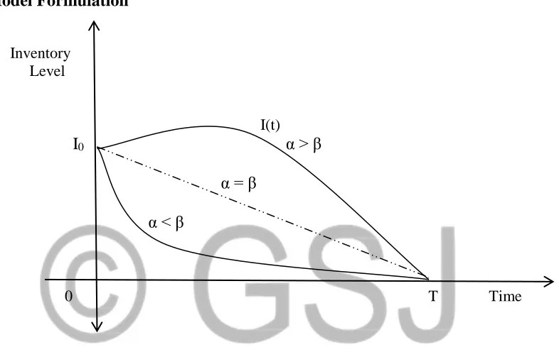
3. Model Formulation
Inventory Level
I(t) I0 α > β
α = β α < β
0 T Time
Figure 1: Inventory movement in an item that is both ameliorating and deteriorating with exponentially increasing demand and linear time dependent holding cost.
From Figure 1, I(t) be the on-hand inventory at time t ≥ 0, then at time t + ∆t, the inventory level in the interval (0 , T) is given by:
at
te t t I t
I t t
I( + )= ( )+( −) ( ) −
(1)
Divide by ∆t and taking limit as ∆t → 0, we have:
ate t I t
I dt
d
− −
=( ) ( ) )
ate t I t
I dt
d − − =−
) ( ) ( )
( (2)
The solution of equation (2) is given by;
t at
Ke a
e t
I( ) ( )
−
+ + − −
= (3)
Now applying the boundary condition at t = 0 and I(t) = I0, I0 is obtained as;
and K is obtained as;
(4)
Substituting equation (4) into equation (3) gives;
t t
at
e
I
e
a
a
e
( )0 ) (
1
−
−
+
+
−
+
+
−
−
=
(5)Apply the boundary conditions, , equation (5) becomes
T T
aT
e
I
e
a
a
e
( )0 )
(
1
0
+
+
−
+
−+
−−
−
=
is thus obtained as follows;
+ − + =
a I
+
−
−
+
−
=
− +a
a
e
I
T a1
) ( 0Substitute the value of I0 into equation (5) to get;
t T a t at e a a e e a a e t
I ( )
) ( ) ( 1 1 ) ( − + − − + − − + − + + − + + − − = t t T a t at e a e a e e a a
e ( ) ( )
) ( )
( 1
1
− − + − − + − − + − + + − + + − − =
a T t at
e e
a− + −
= 1 ( −+) +(−)
(6)
4 Total Amount of On-Hand Inventory during the Complete Cycle:
= TT I t dt
I
0 ( )
− + −= T − + + −
at t T a dt e e a 0 ) ( ) (
1
e dt a dt e a
e a T T t T at
− − + + − = − + − 0 0 ) ( ) ( 1 − + − − − − − + − = − + − a a e a e ae(a )T ( )T 1 1 aT 1
(
)
( ) ( )( 1)
) (
1 − ( ) − − −
+ − −
= aT a− + T aT
e e
e a a
a
(7)
5 Total Demand within (0, T):
RT =
TeatI t dt0 ( )
e dt
a dt e
a
ea T T a t T at
Integrating the above equation we get; − + − − − + − + − = − + + − a e a a e a
e a T a T aT
2 1 1 1 2 ) ( ) (
(
)
(
1)
) ( 2 1 1 ) )( ( 2 ) ( ) ( − + − − − − + + −
= − + a+ − T aT
T a e a a e a a e (8)
6 The Ameliorated Amount within (0, T):
T
T I
A =
(
)
( ) ( )( 1)
) ( ) ( − − − − + − −
= aT a− + T aT
e e
e a a
a
(9)
7 Deteriorated Amount within (0, T):
T
T I
D =
(
)
( ) ( )( 1)
) ( ) ( − − − − + − − +
− T aT
a aT e e e a a
a
(10)
Inventory Holding Cost in a Cycle:
+= T
h t t I t dt
C
0 ( 1 2) ( )
)
(
=
TI t dt+
TtI t dt0 2 0
1 ( ) ( )
(
)
(
)
a TTotal Variable Cost: T CD T CA T t C T C T
TVC = + h( )− T + T
) ( 0
(
)
(
)
(
)
− − − − + − − − + + − − + − − + − + − − − + − − + − − − − + − − + = + − − + − + − ) 1 )( ( ) ( ) ( ) ( ) ( ) ( ) ( ) 1 ( ) ( _ ) 1 ) (( ) ( ) 1 )( ( ) ( ) ( 1 ) ( 2 2 2 2 2 2 ) ( 2 ) ( 2 ) ( 1 0 aT T a aT aT T a T a aT T a aT e e e a a a C a a a a e aT a a e T a e e e e a a a C T To obtain the value of T which minimizes the total variable cost per unit time, we differentiate the above equation with respect to T
(
)
(
)
(
)
(
(
)
)
(
)
(
)
(
)
(
)
− + − + − − + − − + − − − + − − + − − − − − + − − − + − − + − − + − − + + − − − − + − − − + − − + − − = + − + − + − ) ( 1 ) ( ) )( 1 ( ) )( ( ) ( ) ( ) ( ) ( ) 1 ( ) ( ) 1 ) 2 2 (( ) 2 2 ( ) ( 1 ) 1 ( ) ( ) 1 ) (( ) 1 ( ) )( ( 1 ) ( 2 2 2 2 2 2 2 2 2 2 ) 2 2 ( 2 2 2 ) ( 1 0 2 T a aT aT a aT T a aT e T a a e a aT a a C a a T a a a e aT T a a a e T a T a a e aT e T a e aT a a a C TFor optimal cycle period T which minimizes the total variable cost per unit time,
Therefore;
(
)
(
)
(
)
(
(
)
)
(
)
(
)
(
)
(
)
− + − + − − + − − + − − − + − − + − − − − − + − − − + − − + − − + − − + + − − − − + − − − + − − + − − = + − + − + − ) ( 1 ) ( ) )( 1 ( ) )( ( ) ( ) ( ) ( ) ( ) 1 ( ) ( ) 1 ) 2 2 (( ) 2 2 ( ) ( 1 ) 1 ( ) ( ) 1 ) (( ) 1 ( ) )( ( 1 0 ) ( 2 2 2 2 2 2 2 2 2 ) 2 2 ( 2 2 2 ) ( 1 0 2 T a aT aT a aT T a aT e T a a e a aT a a C a a a a a e aT T a a a e T a T a a e aT e T a e aT a a a C TMultiplying through by T2a2(−)2(a− +) we obtain;
10 Economic Order Quantity:
(
)
0) (
1 1
I e
a
EOQ a T − =
+ −
= −+
(13)
11 Numerical Examples
We use equation (12) to obtain the numerical examples below.
Table 1: Input parameter values for the five numerical examples;
a α β C
6 0.23 0.01 200 7000 20 6,000
10 0.4 0.2 200 100,000 2 2,000
13 0.6 0.3 200 50,000 10 1,500
15 0.5 0.3 200 100,000 6 2,500
20 0.8 0.6 150 60,000 20 4,000
Table 2: Output parameter values for the five numerical examples showing the optimal solution obtained;
T* TVC(T)* EOQ*
0.4575 (167 days) 19159 2.26
0.5178 (189 days) 224390 16.21
0.3479 (127 days) 169178 6.46
0.3507 (128 days) 331714 12.06
0.2384 (81 days) 294196 5.61
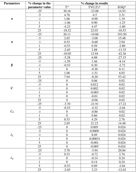
12 Sensitivity Analysis
Table 3: Sensitivity analysis of the second example from Table 3.11.1
Parameters % change in the parameter value
% change in results
T* TVC(T)* EOQ*
a
-25 30.16 -23.08 14.93
-5 4.76 -4.5 2.31
-1 1.06 -0.90 1.19
1 -1.06 0.90 -1.23
5 -4.23 4.47 -1.60
25 -18.52 22.03 -10.53
α
-25 20.11 -19.06 193.50
-5 2.65 -3.08 15.48
-1 0.53 -0.60 2.94
1 -0.53 0.59 -2.80
5 -2.65 2.88 -13.33
25 -10.05 12.94 -42.36
β
-25 -5.28 6.88 -27.15
-5 -1.59 1.46 -8.14
-1 -0.53 0.30 -2.72
1 0 -0.30 0.11
5 1.06 -1.51 6.03
25 7.94 -8.20 53.42
C
-25 0 0.06 0.02
-5 0 0.012 0.02
-1 0 0.002 0.02
1 0 -0.003 0.02
5 0 -0.01 0.02
25 0 -0.06 0.02
-25 -3.70 -21.91 -17.22
-5 -0.53 -4.32 -2.64
-1 0 -0.86 0.02
1 0 0.86 0.02
5 0.53 4.29 2.76
25 2.65 21.23 14.48
-25 0 0.005 0.024
-5 0 0.0009 0.024
-1 0 8.69 0.024
1 0 -0.00031 0.024
5 0 -0.001 0.024
25 0 -0.005 0.024
-25 3.70 -3.94 20.84
-5 0.53 -0.72 2.76
-1 0 -0.14 0.24
1 0 0.14 0.24
5 -0.53 0.69 -2.64
13 Discussion of Results
We use equation 12 to obtain the numerical examples as Table 1 shows the input parameters while Table 2 shows the output values. We then discuss the effect of changes in the values of the parameters on decision variables as contained in Table 3 above. The Table shows that all the decision variables are sensitive to changes in all the parameters. We also notice the following from the table:
• As T* increases, β and increases.
• As TVC(T)* increases, a, α, and increases. • As EOQ* increases, β and increases.
• As T* decreases, a, α and decreases.
• As TVC(T)* decreases, β, C and decreases. • As EOQ* decreases, a, α and decreases.
REFERENCES
1. Moncer H., (1997), Optimal Inventory Policies for Perishable Items with Time-Dependent Demand, International journal of production economics, 50, 35 – 41.
2. Chung K.J. and Tsai S.F., (2001), an Inventory Systems for Deteriorating Items with Shortages and a Linear Trend in Demand-Taking Account of Time Value, Computer Operations Research, 28, 915 – 934.
3. Mishra S.S. and Mishra P.P, (2008), Price Determination for an EOQ Model for Deteriorating Items under Perfect Competition, Computers and Mathematics with Applications, 56, 1082 – 1101.
4. Sahoo N.K., Sahoo C.K. and Sahoo S.K., (2010), An Inventory Model for Constant Deteriorating Items with Price Dependent Demand and Time-varying Holding Cost, International Journal of Computer Science & Communication,1(1), 267 – 271.
5. Singh S., Dube R. and Singh R., (2011), Production Model with Selling Price Dependent Demand and Partial Backlogging under Inflation, International Journal of Mathematical Modelling & Computation, 01, 01 – 07.
6. Khanra S., Ghosh S.K. and Chaudhuri K.S., (2011), an EOQ Model for a Deteriorating Item with Time Dependent Quadratic Demand under Permissible Delay in Payment, Applied Mathematics and Computation, 208, 1 – 9.
8. Chandra (2011), An EOQ Model for Items with Exponential Distribution Deterioration and Linear Trend Deamd Under Permissible Dely in Payments, International Journal of Soft Computing,6(3), 46-53.
9. Mishra S., Raju L.K., Misra U.K.,Misra G., (2012), Optimal Control of an Inventory System with Variable Demand & Ameliorating / Deteriorating Items, Asian Journal of Current Engineering and Maths, 154 – 157, ISSN NO. 2277 – 4920.
10. Deepa K. H., and Khimya S.T., (2013), Stochastic Inventory Model for Ameliorating Items under Supplier’s Trade Credit Policy, International journal of Engineering and Management sciences, 4(2), 203 – 211.
11. Valliathal M., (2013), A Study of Inflation Effects on an EOQ Model for Weibull Deteriorating/Ameliorating Items with Ramp Type of Demand and Shortages, Yugoslav Journal of Operations Research, 23(3), 441 – 455.
12. Barik S., Mishra S., Paikray S.K. and Misra U.K., (2013), An Inventory Model for Weibull Ameliorating, Deteriorating Items under the Influence of Inflation, International Journal of Engineering Research and Applications, 3, 1430 – 1436.
13. Sharma S.C. and Vijay V., (2013), An EOQ Model for Deteriorating Items with Price Dependent Demand, Varying Holding Cost and Shortages under Trade Credit, International Journal of Science and Research, ISSN (Online): 2319-7064.