Efficient Learning Machines

Shelve in Mathematical Sciences User level: Intermediate–Advanced

Effi cient Learning Machines

Machine learning techniques provide cost-effective alternatives to traditional methods for extracting underlying relationships between information and data and for predicting future events by processing existing information to train models. Effi cient Learning Machines explores the major topics of machine learning, including knowledge discovery, classifi cations, genetic algorithms, neural networking, kernel methods, and biologically-inspired techniques.

Mariette Awad and Rahul Khanna’s synthetic approach weaves together the theoretical exposition, design principles, and practical applications of effi cient machine learning. Their experiential emphasis, expressed in their close analysis of sample algorithms throughout the book, aims to equip engineers, students of engineering, and system designers to design and create new and more effi cient machine learning systems. Readers of Effi cient Learning Machines will learn how to recognize and analyze the problems that machine learning technology can solve for them, how to implement and deploy standard solutions to sample problems, and how to design new systems and solutions.

Advances in computing performance, storage, memory, unstructured information retrieval, and cloud computing have coevolved with a new generation of machine learning paradigms and big data analytics, which the authors present in the conceptual context of their traditional precursors. Awad and Khanna explore current developments in the deep learning techniques of deep neural networks, hierarchical temporal memory, and cortical algorithms.

Nature suggests sophisticated learning techniques that deploy simple rules to generate highly intelligent and organized behaviors with adaptive, evolutionary, and distributed properties. The authors examine the most popular biologically-inspired algorithms, together with a sample application to distributed datacenter management. They also discuss machine learning techniques for addressing problems of multi-objective optimization in which solutions in real-world systems are constrained and evaluated based on how well they perform with respect to multiple objectives in aggregate. Two chapters on support vector machines and their extensions focus on recent improvements to the classifi cation and regression techniques at the core of machine learning.

Effi cient Learning Machines systematically guides readers to an understanding and practical mastery of the following techniques:

• The machine learning techniques most commonly used to solve complex real-world problems • Recent improvements to classifi cation and regression techniques

• The application of bio-inspired techniques to real-life problems

• New deep learning techniques that exploit advances in computing performance and storage • Machine learning techniques for solving multi-objective optimization problems with

nondominated methods that minimize distance to the Pareto optimality

Awad

Khanna

For your convenience Apress has placed some of the front

matter material after the index. Please use the Bookmarks

Contents at a Glance

About the Authors ����������������������������������������������������������������������������������������������������

xv

About the Technical Reviewers �����������������������������������������������������������������������������

xvii

Acknowledgments ��������������������������������������������������������������������������������������������������

xix

Chapter 1: Machine Learning

■

��������������������������������������������������������������������������������

1

Chapter 2: Machine Learning and Knowledge Discovery

■

������������������������������������

19

Chapter 3: Support Vector Machines for Classification

■

���������������������������������������

39

Chapter 4: Support Vector Regression

■

����������������������������������������������������������������

67

Chapter 5: Hidden Markov Model

■

_{������������������������������������������������������������������������}

₈₁

Chapter 6: Bioinspired Computing: Swarm Intelligence

■

_{������������������������������������}

₁₀₅

Chapter 7: Deep Neural Networks

■

_{���������������������������������������������������������������������}

₁₂₇

Chapter 8: Cortical Algorithms

■

_{��������������������������������������������������������������������������}

₁₄₉

Chapter 9: Deep Learning

■

_{����������������������������������������������������������������������������������}

₁₆₇

Chapter 10: Multiobjective Optimization

■

_{�����������������������������������������������������������}

₁₈₅

Chapter 11: Machine Learning in Action: Examples

■

_{������������������������������������������}

₂₀₉

Machine Learning

Nature is a self-made machine, more perfectly automated than any automated machine.

To create something in the image of nature is to create a machine, and it was by learning

the inner working of nature that man became a builder of machines.

—Eric Hoffer,

Reflections on the Human Condition

Machine learning (ML) is a branch of artificial intelligence that systematically applies algorithms to synthesize the underlying relationships among data and information. For example, ML systems can be trained on automatic speech recognition systems (such as iPhone’s Siri) to convert acoustic information in a sequence of speech data into semantic structure expressed in the form of a string of words.

ML is already finding widespread uses in web search, ad placement, credit scoring, stock market prediction, gene sequence analysis, behavior analysis, smart coupons, drug development, weather

forecasting, big data analytics, and many more applications. ML will play a decisive role in the development of a host of user-centric innovations.

ML owes its burgeoning adoption to its ability to characterize underlying relationships within large arrays of data in ways that solve problems in big data analytics, behavioral pattern recognition, and information evolution. ML systems can moreover be trained to categorize the changing conditions of a process so as to model variations in operating behavior. As bodies of knowledge evolve under the influence of new ideas and technologies, ML systems can identify disruptions to the existing models and redesign and retrain themselves to adapt to and coevolve with the new knowledge.

The computational characteristic of ML is to generalize the training experience (or examples) and output a hypothesis that estimates the target function. The generalization attribute of ML allows the system to perform well on unseen data instances by accurately predicting the future data. Unlike other optimization problems, ML does not have a well-defined function that can be optimized. Instead, training errors serve as a catalyst to test learning errors. The process of generalization requires classifiers that input discrete or continuous feature vectors and output a class.

The learning process plays a crucial role in generalizing the problem by acting on its historical experience. Experience exists in the form of training datasets, which aid in achieving accurate results on new and unseen tasks. The training datasets encompass an existing problem domain that the learner uses to build a general model about that domain. This enables the model to generate largely accurate predictions in new cases.

Key Terminology

To facilitate the reader’s understanding of the concept of ML, this section defines and discusses some key multidisciplinary conceptual terms in relation to ML.

• classifier. A method that receives a new input as an unlabeled instance of an observation or feature and identifies a category or class to which it belongs. Many commonly used classifiers employ statistical inference (probability measure) to categorize the best label for a given instance.

• confusion matrix (aka error matrix). A matrix that visualizes the performance of the classification algorithm using the data in the matrix. It compares the predicted classification against the actual classification in the form of false positive, true positive, false negative and true negative information. A confusion matrix for a two-class classifier system (Kohavi and Provost, 1998) follows:

Accuracy (AC)= +

+ + +

TP TN

TP TN FN FP (1-1)

Precision (P)= + TP

TP FP (1-2)

Recall R true positive rate

(

,

)

= + TP

TP FN (1-3)

F Measure- =

(

+

)

× × × + b

b 2

2 1 P R

P R , (1-4)

where b has a value from 0 to infinity (∞) and is used to control the weight assigned to P and R.

• cost. The measurement of performance (or accuracy) of a model that predicts (or evaluates) the outcome for an established result; in other words, that quantifies the deviation between predicted and actual values (or class labels). An optimization function attempts to minimize the cost function.

• cross-validation. A verification technique that evaluates the generalization ability of a model for an independent dataset. It defines a dataset that is used for testing the trained model during the training phase for overfitting. Cross-validation can also be used to evaluate the performance of various prediction functions. In k-fold cross-validation,

the training dataset is arbitrarily partitioned into k mutually exclusive subsamples (or folds) of equal sizes. The model is trained k times (or folds), where each iteration uses one of the k subsamples for testing (cross-validating), and the remaining k-1 subsamples are applied toward training the model. The k results of cross-validation are averaged to estimate the accuracy as a single estimation.

• data mining. The process of knowledge discovery (q.v.) or pattern detection in a large dataset. The methods involved in data mining aid in extracting the accurate data and transforming it to a known structure for further evaluation.

• dataset. A collection of data that conform to a schema with no ordering

requirements. In a typical dataset, each column represents a feature and each row represents a member of the dataset.

• dimension. A set of attributes that defines a property. The primary functions of dimension are filtering, classification, and grouping.

• induction algorithm. An algorithm that uses the training dataset to generate a model that generalizes beyond the training dataset.

• instance. An object characterized by feature vectors from which the model is either trained for generalization or used for prediction.

• model. A structure that summarizes a dataset for description or prediction. Each model can be tuned to the specific requirements of an application. Applications in big data have large datasets with many predictors and features that are too complex for a simple parametric model to extract useful information. The learning process synthesizes the parameters and the structures of a model from a given dataset. Models may be generally categorized as either parametric (described by a finite set of parameters, such that future predictions are independent of the new dataset) or nonparametric (described by an infinite set of parameters, such that the data distribution cannot be expressed in terms of a finite set of parameters). Nonparametric models are simple and flexible, and make fewer assumptions, but they require larger datasets to derive accurate conclusions.

• online analytical processing (OLAP). An approach for resolving multidimensional analytical queries. Such queries index into the data with two or more attributes (or dimensions). OLAP encompasses a broad class of business intelligence data and is usually synonymous with multidimensional OLAP (MOLAP). OLAP engines facilitate the exploration of multidimensional data interactively from several perspectives, thereby allowing for complex analytical and ad hoc queries with a rapid execution time. OLAP commonly uses intermediate data structures to store precalculated results on multidimensional data, allowing fast computation. Relational OLAP

(ROLAP) uses relational databases of the base data and the dimension tables. • schema. A high-level specification of a dataset’s attributes and properties. • supervised learning. Learning techniques that extract associations between

independent attributes and a designated dependent attribute (the label). Supervised learning uses a training dataset to develop a prediction model by consuming input data and output values. The model can then make predictions of the output values for a new dataset. The performance of models developed using supervised learning depends upon the size and variance of the training dataset to achieve better generalization and greater predictive power for new datasets. Most induction algorithms fall into the supervised learning category.

• unsupervised learning. Learning techniques that group instances without a prespecified dependent attribute. This technique generally involves learning structured patterns in the data by rejecting pure unstructured noise. Clustering and dimensionality reduction algorithms are usually unsupervised.

Developing a Learning Machine

Machine learning aids in the development of programs that improve their performance for a given task through experience and training. Many big data applications leverage ML to operate at highest efficiency. The sheer volume, diversity, and speed of data flow have made it impracticable to exploit the natural capability of human beings to analyze data in real time. The surge in social networking and the wide use of Internet-based applications have resulted not only in greater volume of data, but also increased complexity of data. To preserve data resolution and avoid data loss, these streams of data need to be analyzed in real time.

The heterogeneity of the big data stream and the massive computing power we possess today present us with abundant opportunities to foster learning methodologies that can identify best practices for a given business problem. The sophistication of modern computing machines can handle large data volumes, greater complexity, and terabytes of storage. Additionally, intelligent program-flows that run on these machines can process and combine many such complex data streams to develop predictive models and extract intrinsic patterns in otherwise noisy data. When you need to predict or forecast a target value, supervised learning is the appropriate choice. The next step is to decide, depending on the target value, between clustering (in the case of discrete target value) and regression (in the case of numerical target value).

You start the development of ML by identifying all the metrics that are critical to a decision process. The processes of ML synthesize models for optimizing the metrics. Because the metrics are essential to developing the solution for a given decision process, they must be selected carefully during conceptual stages.

It is also important to judge whether ML is the suitable approach for solving a given problem. By its nature, ML cannot deliver perfect accuracy. For solutions requiring highly accurate results in a bounded time period, ML may not be the preferred approach. In general, the following conditions are favorable to the application of ML: (a) very high accuracy is not desired; (b) large volumes of data contain undiscovered patterns or information to be synthesized; (c) the problem itself is not very well understood owing to lack of knowledge or historical information as a basis for developing suitable algorithms; and (d) the problem needs to adapt to changing environmental conditions.

The process of developing ML algorithms may be decomposed into the following steps:

1. Collect the data. Select the subset of all available data attributes that might be useful in solving the problem. Selecting all the available data may be unnecessary or counterproductive. Depending upon the problem, data can either be retrieved through a data-stream API (such as a CPU performance counters) or synthesized by combining multiple data streams. In some cases, the input data streams, whether raw or synthetic, may be statistically preprocessed to improve usage or reduce bandwidth.

2. Preprocess the Data. Present the data in a manner that is understood by the consumer of the data. Preprocessing consists of the following three steps:

i. Formatting. The data needs to be presented in a useable format. Using an industry-standard format enable plugging the solution with multiple vendors that in turn can mix and match algorithms and data sources such as XML, HTML, and SOAP.

ii. Cleaning. The data needs to be cleaned by removing, substituting, or fixing corrupt or missing data. In some cases, data needs to be normalized, discretized, averaged, smoothened, or differentiated for efficient usage. In other cases, data may need to be transmitted as integers, double precisions, or strings.

3. Transform the data. Transform the data specific to the algorithm and the knowledge of the problem. Transformation can be in the form of feature scaling, decomposition, or aggregation. Features can be decomposed to extract the useful components embedded in the data or aggregated to combine multiple instances into a single feature.

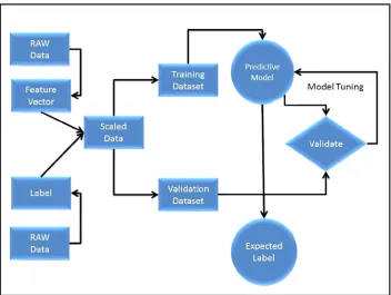
4. Train the algorithm. Select the training and testing datasets from the transformed data. An algorithm is trained on the training dataset and evaluated against the test set. The transformed training dataset is fed to the algorithm for extraction of knowledge or information. This trained knowledge or information is stored as a model to be used for cross-validation and actual usage. Unsupervised learning, having no target value, does not require the training step.

5. Test the algorithm. Evaluate the algorithm to test its effectiveness and performance. This step enables quick determination whether any learnable structures can be identified in the data. A trained model exposed to test dataset is measured against predictions made on that test dataset which are indicative of the performance of the model. If the performance of the model needs improvement, repeat the previous steps by changing the data streams, sampling rates, transformations, linearizing models, outliers’ removal methodology, and biasing schemes.

6. Apply reinforcement learning. Most control theoretic applications require a good feedback mechanism for stable operations. In many cases, the feedback data are sparse, delayed, or unspecific. In such cases, supervised learning may not be practical and may be substituted with reinforcement learning (RL). In contrast to supervised learning, RL employs dynamic performance rebalancing to learn from the consequences of interactions with the environment, without explicit training.

7. Execute. Apply the validated model to perform an actual task of prediction. If new data are encountered, the model is retrained by applying the previous steps. The process of training may coexist with the real task of predicting future behavior.

Machine Learning Algorithms

Based on underlying mappings between input data and anticipated output presented during the learning phase of ML, ML algorithms may be classified into the following six categories:

• Supervised learning is a learning mechanism that infers the underlying relationship between the observed data (also called input data) and a target variable

• Unsupervised learning algorithms are designed to discover hidden structures in unlabeled datasets, in which the desired output is unknown. This mechanism has found many uses in the areas of data compression, outlier detection, classification, human learning, and so on. The general approach to learning involves training through probabilistic data models. Two popular examples of unsupervised learning are clustering and dimensionality reduction. In general, an unsupervised learning dataset is composed of inputs x x x1, 2, 3xn, but it contains neither target outputs

(as in supervised learning) nor rewards from its environment. The goal of ML in this case is to hypothesize representations of the input data for efficient decision making, forecasting, and information filtering and clustering. For example, unsupervised training can aid in the development of phase-based models in which each phase, synthesized through an unsupervised learning process, represents a unique condition for opportunistic tuning of the process. Furthermore, each phase can act as a state and can be subjected to forecasting for proactive resource allocation or distribution. Unsupervised learning algorithms centered on a probabilistic distribution model generally use maximum likelihood estimation (MLE), maximum a posteriori (MAP), or Bayes methods. Other algorithms that are not based on probability distribution models may employ statistical measurements, quantization error, variance preserving, entropy gaps, and so on.

• Semi-supervised learning uses a combination of a small number of labeled and a large number of unlabeled datasets to generate a model function or classifier. Because the labeling process of acquired data requires intensive skilled human labor inputs, it is expensive and impracticable. In contrast, unlabeled data are relatively inexpensive and readily available. Semi-supervised ML methodology operates somewhere between the guidelines of unsupervised learning (unlabeled training data) and supervised learning (labeled training data) and can produce considerable improvement in learning accuracy. Semi-supervised learning has recently gained greater prominence, owing to the availability of large quantities of unlabeled data for diverse applications to web data, messaging data, stock data, retail data, biological data, images, and so on. This learning methodology can deliver value of practical and theoretical significance, especially in areas related to human learning, such as speech, vision, and handwriting, which involve a small amount of direct instruction and a large amount of unlabeled experience.

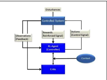
• Reinforcement learning (RL)methodology involves exploration of an adaptive sequence of actions or behaviors by an intelligent agent (RL-agent) in a given environment with a motivation to maximize the cumulative reward (Figure 1-2). The intelligent agent’s action triggers an observable change in the state of the environment. The learning technique synthesizes an adaptation model by training itself for a given set of experimental actions and observed responses to the state of the environment. In general, this methodology can be viewed as a control-theoretic trial-and-error learning paradigm with rewards and punishments associated with a sequence of actions. The RL-agent changes its policy based on the collective experience and consequent rewards. RL seeks past actions it explored that resulted in rewards. To build an exhaustive database or model of all the possible action-reward projections, many unproven actions need to be tried. These untested actions may have to be attempted multiple times before ascertaining their strength. Therefore, you have to strike a balance between exploration of new possible actions and likelihood of failure resulting from those actions. Critical elements of RL include the following:

The

• policy is a key component of an RL-agent that maps the control-actions to the perceived state of the environment.

The

• critic represents an estimated value function that criticizes the actions that are made according to existing policy. Alternatively, the critic evaluates the performance of the current state in response to an action taken according to current policy. The critic-agent shapes the policy by making continuous and ongoing corrections.

The

• reward function estimates the instantaneous desirability of the perceived state of the environment for an attempted control-action.

• Transductive learning (aka transductive inference) attempts to predict exclusive model functions on specific test cases by using additional observations on the training dataset in relation to the new cases (Vapnik 1998). A local model is established by fitting new individual observations (the training data) into a single point in space—this, in contrast to the global model, in which new data have to fit into the existing model without postulating any specific information related to the location of that data point in space. Although the new data may fit into the global model to a certain extent (with some error), thereby creating a global model that would represent the entire problem, space is a challenge and may not be necessary in all cases. In general, if you experience discontinuities during the model development for a given problem space, you can synthesize multiple models at the discontinuous boundaries. In this case, newly observed data are the processed through the model that fulfill the boundary conditions in which the model is valid. • Inductive inference estimates the model function based on the relation of data

to the entire hypothesis space, and uses this model to forecast output values for examples beyond the training set. These functions can be defined using one of the many representation schemes, including linear weighted polynomials, logical rules, and probabilistic descriptions, such as Bayesian networks. Many statistical learning methods start with initial solutions for the hypothesis space and then evolve them iteratively to reduce error. Many popular algorithms fall into this category, including SVMs (Vapnik 1998), neural network (NN) models (Carpenter and Grossberg 1991), and neuro-fuzzy algorithms (Jang 1993). In certain cases, one may apply a lazy learning

Popular Machine Learning Algorithms

This section describes in turn the top 10 most influential data mining algorithms identified by the IEEE International Conference on Data Mining (ICDM) in December 2006: C4.5, k-means, SVMs, Apriori, estimation maximization (EM), PageRank, AdaBoost, k–nearest neighbors (k-NN), naive Bayes, and classification and regression trees (CARTs) (Wu et al. 2008).

C4.5

C4.5 classifiers are one of the most frequently used categories of algorithms in data mining. A C4.5 classifier inputs a collection of cases wherein each case is a sample preclassified to one of the existing classes. Each case is described by its n-dimensional vector, representing attributes or features of the sample. The output of a C4.5 classifier can accurately predict the class of a previously unseen case. C4.5 classification algorithms generate classifiers that are expressed as decision trees by synthesizing a model based on a tree structure. Each node in the tree structure characterizes a feature, with corresponding branches representing possible values connecting features and leaves representing the class that terminates a series of nodes and branches. The class of an instance can be determined by tracing the path of nodes and branches to the terminating leaf.

Given a set S of instances, C4.5 uses a divide-and-conquer method to grow an initial tree, as follows: If all the samples in the list

• S belong to the same class, or if the list S is small, then

create a leaf node for the decision tree and label it with the most frequent class.

Otherwise, the algorithm selects an attribute-based test that branches

• S into multiple

subbranches (partitions) (S1, S2, …), each representing the outcome of the test. The tests are placed at the root of the tree, and each path from the root to the leaf becomes a rule script that labels a class at the leaf. This procedure applies to each subbranch recursively.

Each partition of the current branch represents a child node, and the test separating •

S represents the branch of the tree.

This process continues until every leaf contains instances from only one class or further partition is not possible. C4.5 uses tests that select attributes with the highest normalized information gain, enabling disambiguation of the classification of cases that may belong to two or more classes.

k

-Means

The k-means algorithm is a simple iterative clustering algorithm (Lloyd 1957) that partitions N data points into K disjoint subsets S_j so as to minimize the sum-of-squares criterion. Because the sum of squares is the squared Euclidean distance, this is intuitively the “nearest” mean,

_J=

-Î =

å

å

|x_n | ,

n S j

K

j

j 1

2

m (1-5)

where

x_n= vector representing the nth _{data point}

The algorithm consists of a simple two-step re-estimation process:

1. Assignment: Data points are assigned to the cluster whose centroid is closest to that point.

2. Update: Each cluster centroid is recalculated to the center (mean) of all data points assigned to it.

These two steps are alternated until a stopping criterion is met, such that there is no further change in the assignment of data points. Every iteration requires N × K comparisons, representing the time complexity of one iteration.

Support Vector Machines

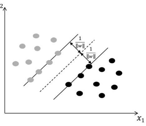
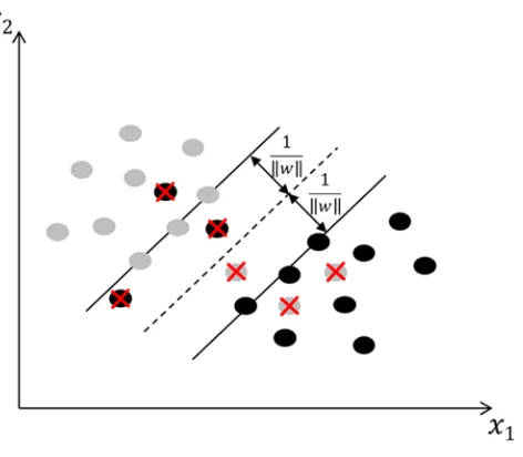
Support vector machines (SVMs) are supervised learning methods that analyze data and recognize patterns. SVMs are primarily used for classification, regression analysis, and novelty detection. Given a set of training data in a two-class learning task, an SVM training algorithm constructs a model or classification function that assigns new observations to one of the two classes on either side of a hyperplane, making it a nonprobabilistic binary linear classifier (Figure 1-3). An SVM model maps the observations as points in space, such that they are classified into a separate partition that is divided by the largest distance to the nearest observation data point of any class (the functional margin). New observations are then predicted to belong to a class based on which side of the partition they fall. Support vectors are the data points nearest to the hyperplane that divides the classes. Further details of support vector machines are given in Chapter 4.

Apriori

Apriori is a data mining approach that discovers frequent itemsets by using candidate generation (Agrawal and Srikant 1994) from a transactional database and highlighting association rules (general trends) in the database. It assumes that any subset of a frequently occurring pattern must be frequent. Apriori performs breadth-first search to scan frequent 1-itemsets (that is, itemsets of size 1) by accumulating the count for each item that satisfies the minimum support requirement. The set of frequent 1-itemsets is used to find the set of frequent 2-itemsets, and so on. This process iterates until no more frequent k-itemsets can be found. The Apriori method that identifies all the frequent itemsets can be summarized in the following three steps:

1. Generate candidates for frequent k + 1-itemsets (of size k + 1) from the frequent

k-itemsets (of size k).

2. Scan the database to identify candidates for frequent k + 1-itemsets, and calculate the support of each of those candidates.

3. Add those itemsets that satisfy the minimum support requirement to frequent itemsets of size k + 1.

Thanks in part to the simplicity of the algorithm, it is widely used in data mining applications. Various improvements have been proposed, notably, the frequent pattern growth (FP-growth) extension, which eliminates candidate generation. Han et al. (Han, Pei, and Yin 2000) propose a frequent pattern tree (FP-tree) structure, which stores and compresses essential information to interpret frequent patterns and uses FP-growth for mining the comprehensive set of frequent patterns by pattern fragment growth. This Apriori technique enhancement constructs a large database that contains all the essential information and compresses it into a highly condensed data structure. In the subsequent step, it assembles a conditional-pattern base which represents a set of counted patterns that co-occur relative to each item. Starting at the frequent header table, it traverses the FP-tree by following each frequent item and stores the prefix paths of those items to produce a conditional pattern base. Finally, it constructs a conditional FP-tree for each of the frequent items of the conditional pattern base. Each node in the tree represents an item and its count. Nodes sharing the same label but residing on different subtrees are conjoined by a node–link pointer. The position of a node in the tree structure represents the order of the frequency of an item, such that a node closer to the root may be shared by more transactions in a transactional database.

Estimation Maximization

The estimation–maximization (EM) algorithm facilitates parameter estimation in probabilistic models with incomplete data. EM is an iterative scheme that estimates the MLE or MAP of parameters in statistical models, in the presence of hidden or latent variables. The EM algorithm iteratively alternates between the steps of performing an expectation (E), which creates a function that estimates the probability distribution over possible completions of the missing (unobserved) data, using the current estimate for the parameters, and performing a maximization (M), which re-estimates the parameters, using the current completions performed during the E step. These parameter estimates are iteratively employed to estimate the distribution of the hidden variables in the subsequent E step. In general, EM involves running an iterative algorithm with the following attributes: (a) observed data, X; (b) latent (or missing) data, Z; (c) unknown parameter, q; and (d) a likelihood function, L(q; X, Z) = P(X, Z|q). The EM algorithm iteratively calculates the MLE of the marginal likelihood using a two-step method:

1. Estimation (E): Calculate the expected value of the log likelihood function, with respect to the conditional distribution of Z, given X under the current estimate of the parameters q(t), such that

2. Maximization (M): Find the parameter that maximizes this quantity:

q(t+ =1) arg max ( | ( )).q Qq q t (1-7)

PageRank

PageRank is a link analysis search algorithm that ranks the elements of hyperlinked documents on the World Wide Web for the purpose of measuring their importance, relative to other links. Developed by Larry Page and Sergey Bin, PageRank produces static rankings that are independent of the search queries. PageRank simulates the concept of prestige in a social network. A hyperlink to a page counts as a vote of support. Additionally, PageRank interprets a hyperlink from source page to target page in such a manner that the page with the higher rank improves the rank of the linked page (the source or target). Therefore, backlinks from highly ranked pages are more significant than those from average pages. Mathematically simple, PageRank can be calculated as

_{r P} r Q

Q

Q Bp

( ) ( )

| |, =

Î

å

(1-8)

where

r(P) = rank of the page P

B_p= the set of all pages linking to page P

|Q| = number of links from page Q r(Q) = rank of the page Q

AdaBoost (Adaptive Boosting)

AdaBoost is an ensemble method used for constructing strong classifiers as linear combinations of simple, weak classifiers (or rules of thumb) (Freund and Schapire 1997). As in any ensemble method, AdaBoost employs multiple learners to solve a problem with better generalization ability and more accurate prediction. The strong classifier can be evaluated as a linear combination of weak classifiers, such that

H x t h xt t

T

( )= × ( ), =

å

b

1 where

H(x) = strong classifier

h_t(x) = weak classifier (feature)

The Adaboost algorithm may be summarized as follows:

Input:

Data-Set I=

{

(

x y1, 1

) (

, x y2, 2

)

,

(

x y3, 3

)

, ,

(

x y_m, _m

)

}

,

Base learning algorithm L Number of learning rounds T

Process:

1 1

i

D

=_m // Initialize weight distribution

FOR (t = 1 to T) DO // Run the loop for t = T iterations

h_t = L(I, D_t) // Train a weak learner h_tfrom I using D_t

Î =t

å

t

-i

t i i i

D

h x y

b_t t t = -Î Î æ è ç ö ø ÷ 1 2 1

ln // calculate the weight of h_t

t

i _t

i

t

y h x

D

D

_Z e t i t i

+

- × ×

= ×

1

(b ( )) _{// Update the distribution,}

// Z_tis the normalization factor

END Output:

H x sign t th x

t T ( )= æ ( ) è ç ö_ø÷ =

å

b 1

// Strong classifier

The AdaBoost algorithm is adaptive, inasmuch as it uses multiple iterations to produce a strong learner that is well correlated with the true classifier. As shown above, it iterates by adding weak learners that are slightly correlated with the true classifier. As part of the adaptation process, the weighting vector adjusts itself to improve upon misclassification in previous rounds. The resulting classifier has a greater accuracy than the weak learners’ classifiers. AdaBoost is fast, simple to implement, and flexible insofar as it can be combined with any classifier.

k

-Nearest Neighbors

The k-nearest neighbors (k-NN) classification methodology identifies a group of k objects in the training set that are closest to the test object and assigns a label based on the most dominant class in this neighborhood. The three fundamental elements of this approach are

an existing set of labeled objects •

a distance metric to estimate distance between objects •

the number of nearest neighbors (

• k)

To classify an unlabeled object, the distances between it and labeled objects are calculated and its

k-nearest neighbors are identified. The class labels of these nearest neighbors serve as a reference for classifying the unlabeled object. The k-NN algorithm computes the similarity distance between a training set, (x, y) ÎI, and the test object, x zˆ =( ˆ, ˆ)x y, to determine its nearest-neighbor list, I_z. x represents the training object, and y represents the corresponding training class. xˆ and yˆ represent the test object and its class, respectively. The algorithm may be summarized as follows:

Input:

Training object (x, y) ÎI and test object x zˆ =( ˆ, ˆ)x y Process:

Compute distance x dˆ =( ˆ, )x x between z and every object (x, y) ÎI. Select IzÍI, the set of k closest training objects to z.

Output (Majority Class):

ˆ arg ( )

( , )

y vmax F v yi

x yi i IZ

= =

∈

∑

F(.) = 1 if argument (.) is TRUE and 0 otherwise, v is the class label.

Naive Bayes

Naive Bayes is a simple probabilistic classifier that applies Bayes’ theorem with strong (naive) assumption of independence, such that the presence of an individual feature of a class is unrelated to the presence of another feature.

Assume that input features x x₁, ₂x_nare conditionally independent of each other, given the class label Y, such that

P x x x Y_n P x Y

i n

i

( ,_{1 2} | )= ( | ) =1

P

(1-9)

For a two-class classification (i = 0,1), we define P(i|x) as the probability that measurement vector x={ ,x x1 2xn}belongs to class i. Moreover, we define a classification score

P x

P x

f x P

f x P

P P j n j j n j j n ( | ) ( | ) ( | ) ( ) ( | ) ( ) ( ) ( ) 1 0 1 1 0 0 1 0 1 1 1 = = = = =

Π

Π

Π

Π

f x f x j j ( | ) ( | ) 1 0 (1-10)

_ln ( | )

( | ) ln ( ) ( ) ln

( | ) ( | ), P x P x P P f x f x j n j j 1 0 1 0 1 0 1 = + =

∑

(1-11)

where P(i|x) is proportional to f(x|i)P(i) and f(x|i) is the conditional distribution of x for class i objects. The naive Bayes model is surprisingly effective and immensely appealing, owing to its simplicity and robustness. Because this algorithm does not require application of complex iterative parameter estimation schemes to large datasets, it is very useful and relatively easy to construct and use. It is a popular algorithm in areas related to text classification and spam filtering.

Classification and Regression Trees

A classification and regression tree (CART) is a nonparametric decision tree that uses a binary recursive partitioning scheme by splitting two child nodes repeatedly, starting with the root node, which contains the complete learning sample (Breiman et al. 1984). The tree-growing process involves splitting among all the possible splits at each node, such that the resulting child nodes are the “purest.” Once a CART has generated a “maximal tree,” it examines the smaller trees obtained by pruning away the branches of the maximal tree to determine which contribute least to the overall performance of the tree on training data. The CART mechanism is intended to yield a sequence of nested pruned trees. The right-sized, or “honest,” tree is identified by evaluating the predictive performance of every tree in the pruning sequence.

Challenging Problems in Data Mining Research

Scaling Up for High-Dimensional Data and High-Speed Data Streams

Designing classifiers that can handle very high-dimensional features extracted through high-speed data streams is challenging. To ensure a decisive advantage, data mining in such cases should be a continuous and online process. But, technical challenges prevent us from computing models over large amounts streaming data in the presence of environment drift and concept drift. Today, we try to solve this problem with incremental mining and offline model updating to maintain accurate modeling of the current data stream. Information technology challenges are being addressed by developing in-memory databases, high-density memories, and large storage capacities, all supported by high-performance computing infrastructure.

Mining Sequence Data and Time Series Data

Efficient classification, clustering, and forecasting of sequenced and time series data remain an open challenge today. Time series data are often contaminated by noise, which can have a detrimental effect on short-term and long-term prediction. Although noise may be filtered, using signal-processing techniques or smoothening methods, lags in the filtered data may result. In a closed-loop environment, this can reduce the accuracy of prediction, because we may end up overcompensating or underprovisioning the process itself. In certain cases, lags can be corrected by differential predictors, but these may require a great deal of tuning the model itself. Noise-canceling filters placed close to the data I/O block can be tuned to identify and clean the noisy data before they are mined.

Mining Complex Knowledge from Complex Data

Complex data can exist in many forms and may require special techniques to extract the information useful for making real-world decisions. For example, information may exist in a graphical form, requiring methods for discovering graphs and structured patterns in large data. Another complexity may exist in the form of non—independent-and-identically-distributed (non-iid) data objects that cannot be mined as an independent single object. They may share relational structures with other data objects that should be identified.

State-of-the-art data mining methods for unstructured data lack the ability to incorporate domain information and knowledge interface for the purpose of relating the results of data mining to real-world scenarios.

Distributed Data Mining and Mining Multi-Agent Data

In a distributed data sensing environment, it can be challenging to discover distributed patterns and correlate the data streamed through different probes. The goal is to minimize the amount of data exchange and reduce the required communication bandwidth. Game-theoretic methodologies may be deployed to tackle this challenge.

Data Mining Process-Related Problems

Autonomous data mining and cleaning operations can improve the efficiency of data mining dramatically. Although we can process models and discover patterns at a fast rate, major costs are incurred by

Security, Privacy, and Data Integrity

Ensuring users’ privacy while their data are being mined is critical. Assurance of the knowledge integrity of collected input data and synthesized individual patterns is no less essential.

Dealing with Nonstatic, Unbalanced, and Cost-Sensitive Data

Data is dynamic and changing continually in different domains. Historical trials in data sampling and model construction may be suboptimal. As you retrain a current model based on new training data, you may experience a learning drift, owing to different selection biases. Such biases need to be corrected dynamically for accurate prediction.

Summary

This chapter discussed the essentials of ML through key terminology, types of ML, and the top 10 data mining and ML algorithms. Owing to the explosion of data on the World Wide Web, ML has found widespread use in web search, advertising placement, credit scoring, stock market prediction, gene sequence analysis, behavior analysis, smart coupons, drug development, weather forecasting, big data analytics, and many more such applications. New uses for ML are being explored every day. Big data analytics and graph analytics have become essential components of cloud-based business development. The new field of data analytics and the applications of ML have also accelerated the development of specialized hardware and accelerators to improve algorithmic performance, big data storage, and data retrieval performance.

References

Agrawal, Rakesh, and Ramakrishnan Srikant. “Fast Algorithms for Mining Association Rules in Large Databases.” In Proceedings of the 20th International Conference on Very Large Data Bases (VLDB ’94), September 12–15, 1994, Santiago de Chile, Chile, edited by Jorge B. Bocca, Matthias Jarke, and Carlo Zaniolo. San Francisco: Morgan Kaufmann (1994): 487–499.

Breiman, Leo, Jerome H. Friedman, Richard A. Olshen, and Charles J. Stone. Classification and Regression Trees. Belmont, CA: Wadsworth, 1984.

Carpenter, Gail A., and Stephen Grossberg. Pattern Recognition by Self-Organizing Neural Networks. Massachusetts: Cambridge, MA: Massachusetts Institute of Technology Press, 1991.

Freund, Yoav, and Robert E. Schapire. “A Decision-Theoretic Generalization of On-Line Learning and an Application to Boosting.” Journal of Computer and System Sciences 55, no. 1 (1997): 119–139.

Han, Jiawel, Jian Pei, and Yiwen Yin. “Mining Frequent Patterns without Candidate Generation.”

In SIGMOD/PODS ’00: ACM international Conference on Management of Data and Symposium on Principles of Database Systems, Dallas, TX, USA, May 15–18, 2000, edited by Weidong Chen, Jeffrey Naughton, Philip A. Bernstein. New York: ACM (2000): 1–12.

Jang, J.-S. R. “ANFIS: Adaptive-Network-Based Fuzzy Inference System.” IEEE Transactions on Systems, Man and Cybernetics 23, no. 3 (1993): 665–685.

Lloyd, Stuart P. “Least Squares Quantization in PCM,” in special issue on quantization, IEEE Transactions on Information Theory, IT-28, no. 2(1982): 129–137.

Samuel, Arthur L. “Some Studies in Machine Learning Using the Game of Checkers,” IBM Journal of Research and Development 44:1.2 (1959): 210–229.

Turing, Alan M. “Computing machinery and intelligence.” Mind (1950): 433–460. Vapnik, Vladimir N. Statistical Learning Theory. New York: Wiley, 1998.

Wu, Xindong, Vipin Kumar, Ross Quinlan, Joydeep Ghosh, Qiang Yang, Hiroshi Motoda,

Machine Learning and Knowledge

Discovery

When you know a thing, to hold that you know it; and when you do not know a thing,

to allow that you do not know it—this is knowledge.

—Confucius,

The Analects

The field of data mining has made significant advances in recent years. Because of its ability to solve complex problems, data mining has been applied in diverse fields related to engineering, biological science, social media, medicine, and business intelligence. The primary objective for most of the applications is to characterize patterns in a complex stream of data. These patterns are then coupled with knowledge discovery and decision making. In the Internet age, information gathering and dynamic analysis of spatiotemporal data are key to innovation and developing better products and processes. When datasets are large and complex, it becomes difficult to process and analyze patterns using traditional statistical methods. Big data are data collected in volumes so large, and forms so complex and unstructured, that they cannot be handled using standard database management systems, such as DBMS and RDBMS. The emerging challenges associated with big data include dealing not only with increased volume, but also the wide variety and complexity of the data streams that need to be extracted, transformed, analyzed, stored, and visualized. Big data analysis uses inferential statistics to draw conclusions related to dependencies, behaviors, and predictions from large sets of data with low information density that are subject to random variations. Such systems are expected to model knowledge discovery in a format that produces reasonable answers when applied across a wide range of situations. The characteristics of big data are as follows:

• Volume: A great quantity of data is generated. Detecting relevance and value within this large volume is challenging.

• Variety: The range of data types and sources is wide.

• Velocity: The speed of data generation is fast. Reacting in a timely manner can be demanding.

• Variability: Data flows can be highly inconsistent and difficult to manage, owing to seasonal and event-driven peaks.

Modern technological advancements have enabled the industry to make inroads into big data and big data analytics. Affordable open source software infrastructure, faster processors, cheaper storage, virtualization, high throughput connectivity, and development of unstructured data management tools, in conjunction with cloud computing, have opened the door to high-quality information retrieval and faster analytics, enabling businesses to reduce costs and time required to develop newer products with customized offerings.

Big data and powerful analytics can be integrated to deliver valuable services, such as these:

• Failure root cause detection: The cost of unplanned shutdowns resulting from unexpected failures can run into billions of dollars. Root cause analysis (RCA) identifies the factors determinative of the location, magnitude, timing, and nature of past failures and learns to associate actions, conditions, and behaviors that can prevent the recurrence of such failures. RCA transforms a reactive approach to failure mitigation into a proactive approach of solving problems before they occur and avoids unnecessary escalation.

• Dynamic coupon system: A dynamic coupon system allows discount coupons to be delivered in a very selective manner, corresponding to factors that maximize the strategic benefits to the product or service provider. Factors that regulate the delivery of the coupon to selected recipients are modeled on existing locality, assessed interest in a specific product, historical spending patterns, dynamic pricing, chronological visits to shopping locations, product browsing patterns, and redemption of past coupons. Each of these factors is weighted and reanalyzed as a function of competitive pressures, transforming behaviors, seasonal effects, external factors, and dynamics of product maturity. A coupon is delivered in real time, according to the recipient’s profile, context, and location. The speed, precision, and accuracy of coupon delivery to large numbers of mobile recipients are important considerations.

• Shopping behavior analysis: A manufacturer of a product is particularly interested in the understanding the heat-map patterns of its competitors’ products on the store floor. For example, a manufacturer of large-screen TVs would want to ascertain buyers’ interest in features offered by other TV manufacturers. This can only be analyzed by evaluating potential buyers’ movements and time spent in proximity to the competitors’ products on the floor. Such reports can be delivered to the manufacturer on an individual basis, in real time, or collectively, at regular intervals. The reports may prompt manufacturers to deliver dynamic coupons to influence potential buyers who are still in the decision-making stage as well as help the manufacturer improve, remove, retain, or augment features, as gauged by buyers’ interest in the competitors’ products.

• Workload resource tuning and selectionin datacenter: In a cloud service management environment, service-level agreements (SLAs) define the expectation of quality of service (QoS) for managing performance loss in a given service-hosting environment composed of a pool of computing resources. Typically, the complexity of resource interdependencies in a server system results in suboptimal behavior, leading to performance loss. A well-behaved model can anticipate demand patterns and proactively react to dynamic stresses in a timely and optimized manner. Dynamic characterization methods can synthesize a self-correcting workload fingerprint codebook that facilitates phase prediction to achieve continuous tuning through proactive workload allocation and load balancing. In other words, the codebook characterizes certain features, which are continually reevaluated to remodel workload behavior to accommodate deviation from an anticipated output. It is possible, however, that the most current model in the codebook may not have been subjected to newer or unidentified patterns. A new workload is hosted on a compute node (among thousands of potential nodes) in a manner that not only reduces the thermal hot spots, but also improves performance by lowering the resource bottleneck. The velocity of the analysis that results in optimal hosting of the workload in real time is critical to the success of workload load allocation and balancing.

Knowledge Discovery

Knowledge extraction gathers information from structured and unstructured sources to construct a knowledge database for identifying meaningful and useful patterns from underlying large and semantically fuzzy datasets. Fuzzy datasets are sets whose elements have a degree of membership. Degree of membership

is defined by a membership function that is valued between 0 and 1.

The extracted knowledge is reused, in conjunction with source data, to produce an enumeration of patterns that are added back to the knowledge base. The process of knowledge discovery involves programmatic exploration of large volumes of data for patterns that can be enumerated as knowledge. The knowledge acquired is presented as models to which specific queries can be made, as necessary. Knowledge discovery joins the concepts of computer science and machine learning (such as databases and algorithms) with those of statistics to solve user-oriented queries and issues. Knowledge can be described in different forms, such as classes of actors, attribute association models, and dependencies. Knowledge discovery in big data uses core machine algorithms that are designed for classification, clustering, dimensionality reduction, and collaborative filtering as well as scalable distributed systems. This chapter discusses the classes of machine learning algorithms that are useful when the dataset to be processed is very large for a single machine.

Classification

Clustering

Clustering is a process of knowledge discovery that groups items from a given collection, based on similar attributes (or characteristics). Members of the same cluster share similar characteristics, relative to those belonging to different clusters. Generally, clustering involves an iterative algorithm of trial and error that operates on an assumption of similarity (or dissimilarity) and that stops when a termination criterion is satisfied. The challenge is to find a function that measures the degree of similarity between two items (or data points) as a numerical value. The parameters for clustering—such as the clustering algorithm, the distance function, the density threshold, and the number of clusters—depend on the applications and the individual dataset.

Dimensionality Reduction

Dimensionality reduction is the process of reducing random variables through feature selection and feature extraction. Dimensionality reduction allows shorter training times and enhanced generalization and reduces overfitting. Feature selection is the process of synthesizing a subset of the original variables for model construction by eliminating redundant or irrelevant features. Feature extraction, in contrast, is the process of transforming the high-dimensional space to a space of fewer dimensions by combining attributes.

Collaborative Filtering

Collaborative filtering (CF) is the process of filtering for information or patterns, using collaborative methods between multiple data sources. CF explores an area of interest by gathering preferences from many users with similar interests and making recommendations based on those preferences. CF algorithms are expected to make satisfactory recommendations in a short period of time, despite very sparse data, increasing numbers of users and items, synonymy, data noise, and privacy issues.

Machine learning performs predictive analysis, based on established properties learned from the training data (models). Machine learning assists in exploring useful knowledge or previously unknown knowledge by matching new information with historical information that exists in the form of patterns. These patterns are used to filter out new information or patterns. Once this new information is validated against a set of linked behavioral patterns, it is integrated into the existing knowledge database. The new information may also correct existing models by acting as additional training data. The following sections look at various machine learning algorithms employed in knowledge discovery, in relation to clustering, classification, dimensionality reduction, and collaborative filtering.

Machine Learning: Classification Algorithms

Logistic Regression

Logistic regression is a probabilistic statistical classification model that predicts the probability of the occurrence of an event. Logistic regression models the relationship between a categorical dependent variable X and a dichotomous categorical outcome or feature Y. The logistic function can be expressed as

P Y X e

e

X X

( | )= .

+

+

+

b b

b b 0 1

0 1

The logistic function may be rewritten and transformed as the inverse of the logistic function—called

logit or log-odds—which is the key to generating the coefficients of the logistic regression,

logit P( ( | )) ln ( | )

( | ) .

Y X P Y X

P Y X X

= -æ è

ç ö

ø

÷ = +

1 b0 b1

(2-2) As depicted in Figure 2-1, the logistic function can receive a range of input values (b₀ +b₁X) between negative infinity and positive infinity, and the output (P(Y |X) is constrained to values between 0 and 1.

Figure 2-1. The logistic function

The logit transform of P(Y |X) provides a dynamic range for linear regression and can be converted back into odds. The logistic regression method fits a regression curve, using the regression coefficients b0 and b₁, as shown in Equation 2-1, where the output response is a binary (dichotomous) variable, and X is numerical. Because the logistic function curve is nonlinear, the logit transform (see Equation 2-2) is used to perform linear regression, in which P(Y |X) is the probability of success (Y) for a given value of X. Using the generalized linear model, an estimated logistic regression equation can be formulated as

logit( (P Y |X X X, , Xn)) kXk.

k n

= = +

=

å

1 1 2 3 0

1

 b b

_(2-3)

The coefficients b₀ and bk (k = 1, 2, ..., n) are estimated, using maximum likelihood estimation (MLE) to model the probability that the dependent variable Y will take on a value of 1 for given values of

X_k (k = 1, 2, ..., n).

Random Forest

Random forest (Breiman 2001) is an ensemble learning approach for classification, in which “weak learners” collaborate to form “strong learners,” using a large collection of decorrelated decision trees (the random forest). Instead of developing a solution based on the output of a single deep tree, however, random forest aggregates the output from a number of shallow trees, forming an additional layer to bagging. Bagging

constructs n predictors, using independent successive trees, by bootstrapping samples of the dataset. The

n predictors are combined to solve a classification or estimation problem through averaging. Although individual classifiers are weak learners, all the classifiers combined form a strong learner. Whereas single decision trees experience high variance and high bias, random forest averages multiple decision trees to improve estimation performance. A decision tree, in ensemble terms, represents a weak classifier. The term

forest denotes the use of a number of decision trees to make a classification decision. The random forest algorithm can be summarized as follows:

1. To construct B trees, select n bootstrap samples from the original dataset.

2. For each bootstrap sample, grow a classification or regression tree.

3. At each node of the tree:

– m predictor variables (or subset of features) are selected at random from all the predictor variables (random subspace).

– The predictor variable that provides the best split performs the binary split on that node.

– The next node randomly selects another set of m variables from all predictor variables and performs the preceding step.

4. Given a new dataset to be classified, take the majority vote of all the B subtrees.

By averaging across the ensemble of trees, you can reduce the variance of the final estimation. Random forest offers good accuracy and runs efficiently on large datasets. It is an effective method for estimating missing data and maintains accuracy, even if a large portion of the data is missing. Additionally, random forest can estimate the relative importance of a variable for classification.

Hidden Markov Model

A hidden Markov model (HMM) is a doubly stochastic process, in which the system being modeled is a Markov process with unobserved (hidden) states. Although the underlying stochastic process is hidden and not directly observable, it can be seen through another set of stochastic processes that produces the sequence of observed symbols. In traditional Markov models, states are visible to an observer, and state transitions are parameterized, using transition probabilities. Each state has a probability distribution over output emissions (observed variables). HMM-based approaches correlate the system observations and state transitions to predict the most probable state sequence. The states of the HMM can only be inferred from the observed emissions—hence, the use of the term hidden. The sequence of output emissions generated by an HMM is used to estimate the sequence of states. HMMs are generative models, in which the joint distribution of observations and hidden states is modeled. To define a hidden Markov model, the following attributes have to be specified (see Figure 2-2):

Set of states: {

• S₁,S₂...,S_n}

Sequence of states:

• Q = q₁,q₂,...,q_t

Markov chain property:

Set of observations:

• O = {o₁,o₂,o₃,...,o_M}

Transition probability matrix:

• P={ },p_ij p_ij=P(q_t+1=S q_j| _t=S_i)

Emission probability matrix:

• B={ ( )},b kj b kj( )=P(xt=o qk| t =Sj) Initial probability matrix:

• p={ },p_i p_i=P(q₁=S_i)

HMM:

• M = (A,B,p)

Figure 2-2. Attributes of an HMM

The three fundamental problems addressed by HMMs can be summarized as follows:

• Model evaluation: Evaluate the likelihood of a sequence of observations for a given HMM (M = (A,B,p)).

• Path decoding: Evaluate the optimal sequence of model states (Q) (hidden states) for a given sequence of observations and HMM model M = (A,B,p).

• Model training: Determine the set of model parameters that best accounts for the observed signal.

HMMs are especially known for their application in temporal pattern recognition, such as speech, handwriting, gesture recognition, part-of-speech tagging, musical score following, partial discharges, and bioinformatics. For further details on the HMM, see Chapter 5.

Multilayer Perceptron

A multilayer perceptron (MLP) is a feedforward network of simple neurons that maps sets of input data onto a set of outputs. An MLP comprises multiple layers of nodes fully connected by directed graph, in which each node (except input nodes) is a neuron with a nonlinear activation function.