balance model from sparse noisy data
Fei Lu1, Nils Weitzel2,3, and Adam H. Monahan4
1Department of Mathematics, Johns Hopkins University, Baltimore, Maryland, USA 2Institut für Umweltphysik, Ruprecht-Karls-Universität Heidelberg, Heidelberg, Germany
3Institut für Geowissenschaften und Meteorologie, Rheinische Friedrich-Wilhelms-Universität Bonn, Bonn, Germany 4School of Earth and Ocean Sciences, University of Victoria, Victoria, British Columbia, Canada
Correspondence:Fei Lu ([email protected])
Received: 8 April 2019 – Discussion started: 23 April 2019
Revised: 8 July 2019 – Accepted: 18 July 2019 – Published: 14 August 2019
Abstract. While nonlinear stochastic partial differential equations arise naturally in spatiotemporal modeling, infer-ence for such systems often faces two major challenges: sparse noisy data and ill-posedness of the inverse problem of parameter estimation. To overcome the challenges, we in-troduce a strongly regularized posterior by normalizing the likelihood and by imposing physical constraints through pri-ors of the parameters and states.
We investigate joint parameter-state estimation by the regularized posterior in a physically motivated nonlinear stochastic energy balance model (SEBM) for paleoclimate reconstruction. The high-dimensional posterior is sampled by a particle Gibbs sampler that combines a Markov chain Monte Carlo (MCMC) method with an optimal particle fil-ter exploiting the structure of the SEBM. In tests using ei-ther Gaussian or uniform priors based on the physical range of parameters, the regularized posteriors overcome the ill-posedness and lead to samples within physical ranges, quan-tifying the uncertainty in estimation. Due to the ill-posedness and the regularization, the posterior of parameters presents a relatively large uncertainty, and consequently, the maximum of the posterior, which is the minimizer in a variational ap-proach, can have a large variation. In contrast, the posterior of states generally concentrates near the truth, substantially filtering out observation noise and reducing uncertainty in the unconstrained SEBM.
1 Introduction
e.g., the last deglaciation and the Holocene by combining indirect observations, so-called proxy data, with physically motivated stochastic models.
The SEBM models surface air temperature, explicitly tak-ing into account sinks, sources, and horizontal transport of energy in the atmosphere, with an additive stochastic forcing incorporated to account for unresolved processes and scales. The model takes the form of a nonlinear SPDE with unknown parameters to be inferred from data. These unknown parame-ters are associated with processes in the energy budget (e.g., radiative transfer, air–sea energy exchange) that are repre-sented in a simplified manner in the SEBM, and may change with a changing climate. The parameters must fall in a pre-scribed range such that the SEBM is physically meaningful. Specifically, they must be in sufficiently close balance for the stationary temperature of the SEBM to be within a physically realistic range. As we will show, the parametric terms aris-ing from this physically based model are strongly correlated, leading to a Fisher information matrix that is ill-conditioned. Therefore, the parameter estimation is an ill-posed inverse problem, and the maximum likelihood estimators of individ-ual parameters have large variations and often fall out of the physical range.
To overcome the ill-posedness in parameter estimation, we introduce a new strongly regularized posterior by normaliz-ing the likelihood and by imposnormaliz-ing the physical constraints through priors on the parameters and the states, based on physical constraints and the climatological distribution. In the regularized posterior, the prior has the same weight as the normalized likelihood to enforce the support of the posterior to be in the physical range. Such a regularized posterior is a natural extension of the regularized cost function in a varia-tional approach: the maximum of the posterior (MAP) is the same as the minimizer of the regularized cost function, but the posterior quantifies the uncertainty in the estimator.
The regularized posterior of the states and parameters is high-dimensional and non-Gaussian. It is represented by its samples, which provide an empirical approximation of the distribution and allow efficient computation of quantities of interest such as posterior means. The samples are drawn us-ing a particle Gibbs sampler with ancestor samplus-ing (PGAS, Lindsten et al., 2014), a special sampler in the family of
par-eters and states within the physical ranges, quantifying the uncertainty in their estimation. Due to the regularization, the posterior of the parameters is supported on a relatively large range. Consequently, the MAP of the parameters has a large variation, and it is important to use the posterior to assess the uncertainty. In contrast, the posterior of the states gen-erally concentrates near the truth, substantially filtering out the observational noise and reducing the uncertainty in state reconstruction.
Tests also show that the regularized posterior is robust to spatial sparsity of observations, with sparser observations leading to larger uncertainties. However, due to the need for regularization to overcome ill-posedness, the uncertainty in the posterior of the parameters can not be eliminated by in-creasing the number of observations in time. Therefore, we suggest alternative approaches, such as re-parametrization of the nonlinear function according to the climatological distri-bution or nonparametric Bayesian inference (see, e.g., Müller and Mitra, 2013; Ghosal and Van der Vaart, 2017), to avoid ill-posedness.
The rest of the paper is organized as follows. Section 2 introduces the SEBM and its discretization, and formulates a state-space model. We also outline in this section the Bayesian approach to the joint parameter-state estimation and the particle MCMC samplers. Section 3 analyzes the ill-posedness of the parameter estimation problem and in-troduces the regularized posterior. The regularized posterior is sampled by PGAS and numerical results are presented in Sect. 4. Discussions and conclusions are presented in Sects. 5 and 6. Technical details of the estimation procedure are de-scribed in Appendix A.
2 State-space model formulation
diffusion with diffusivity ν, while sources and sinks of at-mospheric internal energy are represented by the nonlinear functiongθ(u):
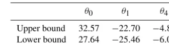
gθ(u)=θ0+θ1u+θ4u4, (2) with the unknown parametersθ. Upper and lower bounds of these three parameters, shown in Table 1, are derived from the energy balance model in Fanning and Weaver (1996), adjusted to current estimates of the Earth’s global energy budget from Trenberth et al. (2009) using appropriate sim-plifications. The equilibrium solution of the SEBM for the average values of the parameters approximates the current global mean temperature closely, and the magnitude of sinks and sources approximates the respective magnitudes in Tren-berth et al. (2009) well. The physical ranges of the param-eters are very conservative and cover current estimates of the global mean temperature during the Quaternary (Snyder, 2016). The state variable and the parameters in the model have been nondimensionalized so that the equilibrium solu-tion of Eq. (1) withf=0 is approximately equal to 1 and 1 time unit represents a year.
The nonlinear functiongθ(u)aggregates parametrizations from Fanning and Weaver (1996) for incoming short-wave radiation, outgoing long-wave radiation, radiative air–surface flux, sensible air–surface heat flux, and the latent heat flux into the atmosphere according to their polynomial order. The quartic nonlinearity of the function gθ(u) arises from the
Stefan–Boltzmann dependence of long-wave radiative fluxes on atmospheric temperature, while a linear feedback is in-cluded to represent state dependence of, e.g., surface energy fluxes and albedo. Inclusion of quadratic and cubic nonlin-earities in gθ(u) (to account for nonlinearities in the feed-backs just noted) was found to exacerbate the ill-posedness of the model without qualitatively changing the character of the model dynamics within the parameter range appropriate for the study of Quaternary climate variability (e.g., without ad-mitting multiple deterministic equilibria associated with the ice–albedo feedback). In reality, the diffusivityνand the pa-rametersθj,j=(0,1,4)will depend on latitude, longitude,
and time. We will neglect this complexity in our idealized analysis.
The stochastic termf (t, ξ ), which models the net effect of unresolved or oversimplified processes in the energy budget, is a centered Gaussian field that is white in time and colored
Ef (t, ξ )f (s, η)=δ(t−s)C(|ξ−η|), (3) with the covariance kernelC(r)being the Matérn covariance kernel given by
Cα(r)=σf2 21−α
0(α) √
2αr ρ
α Kα
√ 2αr
ρ
, (4)
where0is the gamma function,ρis a scaling factor, andKα
is the modified Bessel function of the second kind. We fo-cus on the estimation of the parametersθ and assume thatν
and the parameters off are known. Estimatingνin energy balance models with data assimilation methods is studied in Annan et al. (2005), whereas estimation of parameters offin the context of linear SPDEs is covered for example in Lind-gren et al. (2011).
In a paleoclimate context, temperature observations are sparse (in space and time) and derived from climatic prox-ies, such as pollen assemblages, isotopic compositions, and tree rings, which are indirect measures of the climate state. To simplify our analysis, we neglect the potentially nonlinear transformations associated with the proxies and focus on the effect of observational sparseness. This is a common strategy in the testing of climate field reconstruction methods (e.g., Werner et al., 2013). As such, we take the data to be noisy observations of the solution atdolocations:
yi(t )=Hi(u(t ))+i(t )=u(t, ξi)+i(t ), (5)
fori=1, . . ., do, where eachξi∈ [−π, π] × [−π/2, π/2]is
a location of observation,His the observation operator, and
i(t )∼N(0, σ2)are independent identically distributed (iid) Gaussian noise. The data are sparse in the sense that only a small number of the spatial locations are observed.
2.2 State-space model representation
variance Rdescribed in more detail in Eq. (A19). Here the subscriptnis a time index. Therefore, the transition proba-bility densitypθ(un+1|un), the probability density ofUn+1 conditional onUnandθ, is
pθ(un+1|un)=det(2πR)−1/2
exp
−(un+1−µθ(un))
TR−1(u
n+1−µθ(un))
2
. (7)
2.2.2 The observation model
In discrete form, we assume that the locations of observa-tion are the nodes of the finite elements. Then the obser-vation function in Eq. (5) is simply Hi(Un)=Un,ki, with
ki ∈ {1, . . ., d}denoting the index of the node under
obser-vation, for i=1, . . ., d0, and we can write the observation model as
Yn=HUn+n, yn∈Rdo, (8) whereH∈Rdo×dbis called the observation matrix and{
n}is a sequence of iid Gaussian noise with distributionN(0,Q), where Q=Diag{σi2}. Equivalently, the probability of ob-servingyngiven stateUnis
p(yn|Un)=det(2πQ)−1/2 exp
−(yn−HUn)
TQ−1(y
n−HUn) 2
. (9)
2.3 Bayesian inference for SSM
Given observations y1:N:=(y1, . . ., yN), our goal is to jointly estimate the state U1:N:=(U1, . . ., UN)and the pa-rameter vector θ:=(θ0, θ1, θ4) in the state-space model Eqs. (6)–(9). The Bayesian approach estimates the joint dis-tribution of (U1:N, θ ) conditional on the observations by
drawing samples to form an empirical approximation of the high-dimensional posterior. The empirical posterior ef-ficiently quantifies the uncertainty in the estimation. There-fore, the Bayesian approach has been widely used (see the review of Kantas et al., 2009, and the references therein).
parameterθ, which can be explicitly derived from the obser-vation model Eq. (8):
pθ(y1:N|u1:N)=p(y1:N|u1:N)=
Y
n
p(yn|un), (11) withp(yn|un)given in Eq. (9). Finally, the probability den-sity function of the stateU1:N given parameterθcan be
de-rived from the state model Eq. (6):
pθ(u1:N)=pθ(u1)
N−1 Y
n=1
pθ(un+1|un), (12)
withpθ(un+1|un)specified by Eq. (7).
2.4 Sampling the posterior by particle MCMC methods In practice, we are interested in the expectation of quantities of interest or the probability of certain events. These com-putations involve integrations of the posterior that can nei-ther be computed analytically nor by numerical quadrature methods due to the curse of dimensionality: the posterior is a high-dimensional non-Gaussian distribution involving vari-ables with a dimension at the scale of thousands to millions. Monte Carlo methods generate samples to approximate the posterior by the empirical distribution, so that quantities of interest can be computed efficiently.
MCMC methods are popular Monte Carlo methods (see, e.g., Liu, 2001) that generate samples along a Markov chain with the posterior as the invariant measure. For joint distribu-tions of parameters and states, a standard MCMC method is Gibbs sampling which consists of alternatively updating the state variableU1:Nconditional onθandy1:Nby sampling p(u1:N|θ, y1:N)=
pθ(u1:N)pθ(y1:N|u1:N) pθ(y1:N)
(13) and then updating the parameter θ conditional on U1:N= u1:Nby sampling the marginal posterior ofθ:
p(θ|u1:N, y1:N)=p(θ|u1:N)=p(θ )pθ(u1:N). (14)
Due to the high dimensionality ofU1:N, a major difficulty
in sampling p(u1:N|θ, y1:N) is the design of efficient
pro-posal densities that can effectively explore the support of
(2010) provide a framework for systematically combin-ing SMC methods with MCMC methods, exploitcombin-ing the strengths of both techniques. In the particle MCMC sam-plers, SMC algorithms provide high-dimensional proposal distributions, and Markov transitions guide the SMC ensem-ble to sufficiently explore the target distribution. The transi-tion is realized by a conditransi-tional SMC technique, in which a reference trajectory from the previous step is kept throughout the current step of SMC sampling.
In this study, we sample the posterior by PGAS (Lind-sten et al., 2014), a particle MCMC method that enhances the mixing of the Markov chain by sampling the ancestor of the reference trajectory. For the SMC, we use an optimal particle filter, which takes advantage of the linear Gaussian observation model and the Gaussian transition density of the state variables in our current SEBM. More generally, when the observation model is nonlinear and the transition density is non-Gaussian, the optimal particle filter can be replaced by implicit particle filters (Chorin and Tu, 2009; Morzfeld et al., 2012) or local particle filters (Penny and Miyoshi, 2016; Poterjoy, 2016; Farchi and Bocquet, 2018); we refer the reader to Carrassi et al. (2018), Law et al. (2015), and Vetra-Carvalho et al. (2018) for other data assimilation tech-niques. The details of the algorithm are provided in Sect. A3.
3 Ill-posedness and regularized posteriors
In this section, we first demonstrate and then analyze the fail-ure of standard Bayesian inference of the parameters with the posteriors in Eq. (10). The standard Bayesian inference of the parameters fails in the sense that the posterior Eq. (10) tends to have a large probability mass at non-physical pa-rameter values. In the process of approximating the posterior by samples, the values of these samples often either hit the (upper or lower) bounds in Table 1 when we use a uniform prior or exceed these bounds when we use a Gaussian prior. As we shall show next, the standard Bayesian inverse prob-lem isnumerically ill-posedbecause the Fisher information matrix is ill-conditioned, which makes the inference numeri-cally unreliable. Following the idea of regularization in vari-ational approaches, we propose using regularized posteriors in the Bayesian inference. This approach unifies the Bayesian and variational approaches: the MAP is the minimizer of the regularized cost function in the variational approach, but the
discretization.
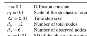
ν=0.1 Diffusion constant
σf=0.1 Scale of the stochastic forcing 1t=0.01 Time step size
db=12 Number of total nodes do=6 Number of observed nodes σ=0.01 SD of the observation noise
Bayesian approach quantifies the uncertainty of the estimator by the posterior.
3.1 Model settings and tests
Based on the physical upper and lower bounds in Table 1, we consider two priors for the parameters: a uniform distribu-tion on these intervals and a Gaussian distribudistribu-tion centered at the median and with 3 standard deviations in the interval, as listed in Table 2.
Throughout this study, we shall consider a relatively small numerical mesh for the SPDE with only 12 nodes for the finite elements. Such a small mesh provides a toy model that can neatly represent the spatial structure on the sphere while allowing for systematic assessments of statistical prop-erties of the Bayesian inference with moderate computa-tional costs. Numerical tests show that the above FEM semi-backward Euler scheme is stable for a time step size
1t=0.01 and a stochastic forcing with scaleσf=0.1 (see Sect. A1 for more details about the discretization). A typical realization of the solution is shown in Fig. 1 (panels a and b), where we present the solution on the sphere at a fixed time with the 12-node finite-element mesh, as well as the trajecto-ries of all 12 nodes.
The standard deviation of the observation noise is set to σ=0.01, i.e., 1 order of magnitude smaller than the stochastic forcing and 2 orders of magnitude smaller than the climatological mean.
Figure 1.A typical realization of the solution to the SEBM.(a)The solution at time stepn=10 on the sphere with the 12-node finite-element mesh.(b)The trajectories of all 12 nodes over 100 time steps.(c)Histogram estimates of the climatological probability distribution of all nodes of the true states (salmon) and the observations (blue).
1 and vary mostly in the interval[0.92,1.05]. We shall use a Gaussian approximation based on the climatological distri-bution of the partial noisy observations as a prior to constrain the state variables.
We summarize the settings of numerical tests in Table 3. 3.2 Ill-posedness of the standard Bayesian inference of
parameters
By the Bernstein–von Mises theorem (see, e.g., Van der Vaart, 2000, chap. 10), the posterior distribution of the pa-rameters conditional on the true state data approaches the likelihood distribution as the data size increases. That is,
p(θ|u1:N)in Eq. (14) becomes close to the likelihood
dis-tribution p(u1:N|θ )(which can be viewed as a distribution
of θ) as the data size increases. Therefore, if the likelihood distribution is numerically degenerate (in the sense that some components are undetermined), then the Bayesian posterior will also become close to degenerate, so that the Bayesian in-ference for parameter estimation will be ill-posed. In the fol-lowing, we show that for this model the likelihood is degen-erate even if the full states are observed with zero observa-tion noise and that the maximum likelihood estimators have large nonphysical fluctuations (particularly when the states are noisy). As a consequence, the standard Bayesian param-eter inference fails by yielding nonphysical samples.
We show first that the likelihood distribution is numeri-cally degenerate because the Fisher information matrix is ill-conditioned. Following the transition density Eq. (7), the log likelihood of the state{u1:N}is
l(θ, u1:N)=c−
1 2
N X
n=1
(un+1−µθ(un))TR−1
(un+1−µθ(un)), (15)
wherecis a constant independent of(θ, u1:N). Sinceµθ(·)is
linear inθ(cf. Eq. A19), the likelihood function is quadratic
inθand the corresponding scaled Fisher information matrix is
FN=
1
N N X
n=1
Gθ,k(un)TR−1Gθ,l(un) !
k,l=0,1,4
, (16)
where the vectors Gθ,k(un)∈Rdb are defined in
Eq. (A20). As N→ ∞, the Fisher information matrix converges, by ergodicity of the system, to its expectation
1t σf−2E[(Aun)◦kATTCTCAT(Aun)◦l]
k,l=0,1,4, where the matrices A, AT andC, arising in the spatial–temporal
discretization, are defined in Sect. A1. Intuitively, ne-glecting these matrices and viewing the vector un as
a scalar, this expectation matrix could be reduced to
(1t σf−2E[uknuln])k,l=0,1,4, which is ill-conditioned because un has a distribution concentrated near 1 with a standard deviation at the scale of 10−2(see Fig. 1).
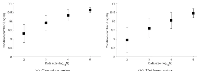
Figure 2 shows the means and standard deviations of the condition numbers (the ratio between the maximum and the minimum singular values) of the Fisher information matrices from 100 independent simulations. Each of these simulations generates a long trajectory of length 105using a parameter drawn randomly from the prior and computes the Fisher in-formation matrices using the true trajectory of all 12 nodes, for subsamples of lengthsN ranging from 102 to 105. For both the Gaussian and uniform priors, the condition numbers are on the scale of 108–1011and therefore the Fisher infor-mation matrix is ill-conditioned. In particular, the condition number increases as the data size increased, due to the ill-posedness of the inverse problem of parameter estimation.
The ill-conditioned Fisher information matrix leads to highly variable maximum likelihood es-timators (MLEs), computed from FNθ=bN with bN= 1
N
PN
n=1Gθ,k(un)TR−1(un+1−M−1t1M0un)
Figure 2.The mean and standard deviation of the condition numbers of the Fisher information matrices, computed using true trajectories, out of 100 simulations of length ranging fromN=102to 105. The condition numbers are at the scale of 108–1011, indicating that the Fisher information matrix is ill-conditioned.
The ill-posedness is particularly problematic when{u1:N}
is observed with noise, as the ill-conditioned Fisher informa-tion matrix amplifies the noise in observainforma-tions and leads to nonphysical estimators. Figure 3 shows the means and stan-dard deviations of errors of MLEs computed from true and noisy trajectories in 100 independent simulations. In each of these simulations, the “noisy” trajectory is obtained by adding a white noise with standard deviation σ=0.01 to
a “true” trajectory generated from the system with a true pa-rameter randomly drawn from the prior. For both Gaussian and uniform priors, the standard deviations and means of the errors of the MLE from the noisy trajectories are 1 order of magnitude larger than those from true trajectories. In partic-ular, the variations are large when the data size is small. For example, whenN=100, the standard deviation of the MLE forθ0from noisy observations is on the order of 103, 2 orders of magnitude larger than its physical range in Table 2.
The standard deviations decrease as the data size increases, at the expected rate of 1/
√
N. However, the errors are too large to be practically reduced by increasing the size of the data: for example, a data sizeN=1010 is needed to reduce the standard deviation ofθ4to less than 0.1 (which is about 10 % the size of the physical range[−6.00,−4.80]as spec-ified in Table 2). In summary, the ill-posedness leads to pa-rameter estimators with large variations that are far outside the physical ranges of the parameters.
3.3 Regularized posteriors
To overcome the ill-posedness of the parameter estimation problem, we introduce strongly regularized posteriors by normalizing the likelihood function. In addition, to prevent unphysical values of the states, we further regularize the state variables in the likelihood by an uninformative climatologi-cal prior. That is, consider theregularized posterior:
pN(θ, u1:N|y1:N)=
1
Zp(θ ) pc(u
1:N)pθ(u1:N)pθ(y1:N|u1:N)
pθ(y1:N)
1/N
, (17)
where Z:=Rp(θ )hpc(u1:N)pθ(u1:N)pθ(y1:N|u1:N)
pθ(y1:N)
i1/N
dθdu1:N
is a normalizing constant andpc(u1:N) is the prior of the
states estimated from a Gaussian fit to climatological statis-tics of the observations, neglecting correlations. That is, we setpc(u1:N)as
pc(u1:N):= N Y
n=1 1 2π σdb
c
exp
−|un−uc| 2 2σ2
c
, (18)
withσc=2 p
σ2
o−σ2, whereuc and σo are the mean and
standard deviation of the observations over all states. Here the multiplicative factor 2 aims for a larger band to avoid an overly narrow prior for the states.
This prior can be viewed as a joint distribution of the state variables assuming all components are independent identi-cally Gaussian distributed with mean uc and variance σc2. Clearly, it uses the minimum amount of information about the state variables, and we expect it can be improved by tak-ing into consideration spatial correlations or additional field knowledge in practice.
The regularized posterior can be viewed as an extension of the regularized cost function in the variational approach. In fact, the negative logarithm of the regularized posterior is the same (up to a multiplicative factor N1 and an additive constant logZ− 1
Nlogpθ(y1:N)) as the cost function in
vari-ational approaches with regularization. More precisely, we have
−logpN(θ, u1:N|y1:N)=
1
NCy1:N(θ, u1:N)
+logZ− 1
N logpθ(y1:N), (19)
whereCy1:N(θ, u1:N)is the cost function with regularization:
Cy1:N(θ, u1:N)= −
N X
n=1 log
p(un|un−1, θ )p(yn|un)
Figure 3.The standard deviations and means of the errors of the MLEs, computed from true and noisy trajectories, out of 100 independent simulations with true parameters sampled from the Gaussian and uniform priors. In all cases, the deviations and biases (i.e., means of errors) are large. In particular, in the case of noisy observations, the deviations are on orders ranging from 10 to 1000, far beyond the physical ranges of the parameters in Table 1. Though the deviations decrease as data size increases, an impractically large data size is needed to reduce them to a physical range. Also, the means of errors are larger than the size of physical ranges of the parameters, with values that decay slowly as data size increases.
When the prior is Gaussian, the regularization corresponds to Tikhonov regularization. Therefore, the regularized posterior extends the regularized cost function to a probability distri-bution, with the MAP being the minimizer of the regularized cost function.
The regularized posterior normalizes the likelihood by an exponent 1/N. This normalization allows for a larger weight (more trust) on the prior, which can then suffi-ciently regularize the singularity in the likelihood and there-fore reduces the probability of nonphysical samples. In-tuitively, it avoids the shrinking of the likelihood as the data size increases. When the system is ergodic, the sum
1
N PN
n=1log
pθ(un|un−1)p(yn|un)
converges to the spatial average E[logpθ(Un|Un−1)p(yn|Un)] with respect to the
invariant measure asNincreases. While being effective, this factor may not be optimal (O’Leary, 2001), and we leave the exploration of optimal regularization factors to future work.
In the sampling of the regularized posterior, we update the state variable U1:N conditional onθ andy1:N by
sam-plingpc(u1:N)pθ(u1:N|θ, y1:N)(withpθ(u1:N|θ, y1:N)
spec-ified in Eq. 13) using SMC methods. Compared to the stan-dard PMCMC algorithm outlined in Sect. 2.4, the only dif-ference occurs when we update the parameterθ conditional on the estimated statesu1:N. Instead of Eq. (14), we draw a
sample ofθfrom the regularized posterior
pN(θ|u1:N, y1:N) ∝ p(θ )[pθ(u1:N)]1/N. (21)
4 Bayesian inference with regularized posteriors The regularized posteriors are approximated by the empirical distribution of samples drawn using particle MCMC
meth-ods, specifically PGAS (see Sect. A3) in combination with SMC using optimal importance sampling (see Sect. A2). In the following section, we first diagnose the Markov chain and choose a reasonable chain length for subsequent analyses. We then present the results of parameter estimation and state estimation.
In all the tests presented in this study, we use onlyM=5 particles for the SMC, as we can be confident of the Markov chain produced by the particle MCMC methods converging to the target distribution based on theoretical results (see An-drieu et al., 2010; Lindsten et al., 2014). In general, the more particles are used, the better the SMC algorithm (and hence the particle MCMC methods) will perform, at the price of increased computational cost.
4.1 Diagnosis of the Markov chain Monte Carlo algorithm
To ensure that the Markov chain generated by PGAS is well-mixed and to find a length for the chain such that the poste-rior is acceptably approximated, we shall assess the Markov chain by three criteria: the update rate of states; the corre-lation length of the Markov chain; and the convergence of the marginal posteriors of the parameters. These empirical criteria are convenient and, as we discuss below, have found to be effective in our study. We refer to Cowles and Carlin (1996) for a detailed review of various criteria for diagnos-ing MCMC.
The update rate of states is computed at each time of the state trajectoryu1:Nalong the Markov chain. That is, at each
Figure 4.The update rate of the states at different times along the trajectory. The high update rate at timet=1 is due to the initialization of the particles near the equilibrium and the ancestor sampling. The high update rate at the end time is due to the nature of the SMC filter. Note that the uniform prior has update rates close to 1 at all times.
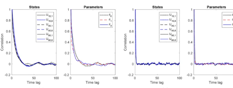
Figure 5. The empirical autocorrelation functions (ACFs) of the Markov chain of parameters(θ0, θ1, θ4)and states Un,k at timesn=
{1040,90}and nodesk= {1,8}, computed from a Markov chain with length 10 000. The ACFs fall within a threshold of 0.1 around zero within a time lag of about 25 for the Gaussian prior, and a time lag of about 5 for the uniform prior.
The update rate measures the mixing of the Markov chain. In general, an update rate above 0.5 is preferred, but a high rate close to 1 is not necessarily the best. Figure 4 shows the up-date rates of typical simulations for both the Gaussian prior and the uniform prior. For both priors, the update rates are above 0.5, indicating a fast mixing of the chain. The rates tend to increase with time (except for the first time step) to a value close to 1 at the end of the trajectory. This phenomenon agrees with the particle depletion nature of the SMC filter: when tracing back in time to sample the ancestors, there are fewer particles and therefore the update rate is lower. The high update rate at the timet=1 step is due to our initial-ization of the particles near the equilibrium, which increases the possibility of ancestor updates in PGAS. We also note that the uniform prior has update rates close to 1 at all times, much higher than the rates of the Gaussian prior. Higher up-date rates occur for the uniform prior because the deviations of parameter samples from the previous values are larger, re-sulting in an increased probability of updating the reference trajectory in the conditional SMC.
Table 4.The settings of the particle MCMC using SMC with opti-mal importance densities.
M=5 Number particles in SMC L=104 Length of the Markov chain
N=100 Number of time steps of observations.
We test the correlation length of the Markov chain by find-ing the smallest lag at which the empirical autocorrelation functions (ACFs) of the states and the parameters are close to zero.
Figure 6.The empirical marginal distributions of the samples from the posterior as the length of the Markov chain increases. Note that the marginal posteriors converge rapidly as the length of the chain increases. In particular, a chain with length 1000 provides a reasonable approximation to the posterior, capturing the shape and spread of the distribution.
The relatively small decorrelation length of the Markov chain indicates that we can accurately approximate the pos-terior by a chain of a relatively short length. This result is demonstrated in Fig. 6, where we plot the empirical marginal posteriors of the parameters, using Markov chains of three different lengths:L=1000,5000, and 10 000. The marginal posteriors withL=1000 are reasonably close to those with
L=104, and those with L=5000 are almost identical to those with L=104. In particular, the marginal posteriors withL=103capture the shape and spread of the distribu-tions for L=104. Therefore, a Markov chain with length
L=104provides a reasonably accurate approximation of the posterior. Hence, we use Markov chains with lengthL=104 in all simulations from here on. This choice of chain length may be longer than necessary, but allows for confidence that the results are robust.
In summary, based on the above diagnosis of the Markov chain generated by PMCMC, to run many simulations for statistical analysis of the algorithm within a limited compu-tation cost, we use chains with length L=104to approxi-mate the posterior. For the SMC algorithm, we use only five particles. The number of observations in time isN=100. 4.2 Parameter estimation
One of the main goals in Bayesian inference is to quantify the uncertainty in the parameter-state estimation by the pos-terior. We access the parameter estimation by examining the samples of the posterior in a typical simulation, for which we consider the scatter plots and marginal distributions, the MAP, and the posterior mean. We also examine the statistics of the MAP and the posterior mean in 100 independent sim-ulations. In each simulation, the parameters are drawn from the prior distribution ofθ. Then, a realization of the SEBM is
simulated. Finally, observations are created by applying the observation model to the SEBM realization.
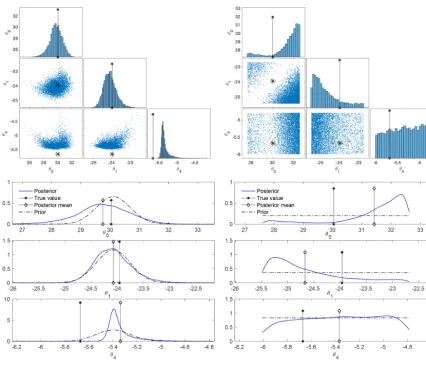
The empirical marginal posteriors of the parametersθ=
(θ0, θ1, θ4)in two typical simulations, for the Gaussian and uniform priors, are shown in Fig. 7. The top row presents scatter plots of samples along with the true values of the pa-rameters (asterisks) and the bottom row presents the marginal posteriors for each parameter in comparison with the priors.
In the case of the Gaussian prior, the scatter plots show a posterior that is far from Gaussian, with clear nonlinear de-pendence betweenθ0and the other parameters. The marginal posteriors ofθ0andθ1 are close to their priors, with larger tails (to the left forθ0and to the right forθ1). The marginal distribution ofθ4 concentrates near the center of the prior with a larger tail to the right. The posterior has the most prob-ability mass near the true values ofθ0andθ1, which are in the high-probability region of the prior. However, it has no probability mass near the true value ofθ4– which is of a low probability in the prior.
In the case of the uniform prior, the scatter plots show a concentration of probability near the boundaries of the phys-ical range. The marginal posteriors ofθ0andθ1clearly devi-ate from the priors, concentrating near the parameter bounds (the upper bound forθ0and the lower bound for θ1 in this realization); the marginal posterior ofθ4is close to the prior, with slightly more probability mass for large values.
Figure 7.Posteriors of the parameters in a typical simulation, with both the Gaussian and the uniform prior. The true values of the parameters, as well as the data trajectory, are the same for both priors. The top row displays scatter plots of the samples (blue dots), with the true values of the parameters shown by asterisks. The bottom row displays the marginal posteriors (blue lines) of each component of the parameters and the priors (black dash-dot lines), with the posterior mean marked by diamonds and the true values marked by asterisks. The posterior correlations areρ01=0.20,ρ04= −0.19, andρ14=0.57 in the case of the Gaussian prior andρ01= −0.23,ρ04= −0.01, andρ14= −0.05 in the case of the uniform prior.
The non-Gaussianity of the posterior (including the con-centration near the boundaries), its insensitivity to changes in the true parameter, and its limited reduction of uncertainty from the prior (Figs. 7–8) are due to the degeneracy of the likelihood distribution and to the strong regularization. Re-call that the degenerate likelihood leads to MLEs with large variations and biases, with the standard deviation of the es-timators ofθ0andθ1being about 10 times larger than those ofθ4(see Fig. 3). As a result, when regularized by the Gaus-sian prior, the componentsθ0andθ1, which are more under-determined by the likelihood, are constrained mainly by the Gaussian prior, and therefore their marginal posteriors are close to their marginal priors. In contrast, the componentθ4 is forced to concentrate around the center of the prior but with a large tail. While dramatically reducing the large uncertainty ofθ0andθ1in the ill-conditioned likelihood, the regularized
posterior still exhibits a slightly larger uncertainty than the prior for these two components.
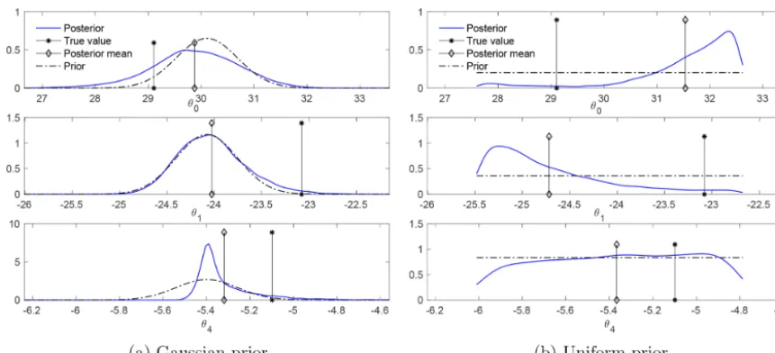
varia-Figure 8.The marginal posteriors with a different set of true values for the parameters. The marginal posteriors change little from those in Fig. 7.
tions, but the correlations betweenθ4andθ0as well asθ1are weakened (Fig. 7).
In practice, one is often interested in a point estimate of parameters. Commonly used point estimators are the MAP and the posterior mean. Figures 7–8 show that both the MAP and the posterior mean can be far away from the truth for Gaussian as well as uniform priors. In particular, in the case of the uniform prior, the MAP values are further away from the truth than the posterior mean. In the case of the Gaussian prior, the MAP values do not present a clear advantage or disadvantage over the posterior mean.
Table 5a shows the means and standard deviations of the errors of the posterior mean and MAP from 100 independent simulations. In each simulation and for each prior, we drew a parameter sample from the prior and generated a trajec-tory of observations, and then estimated jointly the parame-ters and states. The table shows that both posterior mean and MAP estimates are generally biased, consistent with the bi-ases in Figs. 7 and 8. More specifically, in the case of the Gaussian prior, the MAP has slightly smaller biases than the posterior mean, but the two have almost the same variances. Both are negatively biased for θ0and slightly positively bi-ased forθ1andθ4. In the case of the uniform prior, the MAP features biases and standard deviations which are about 50 % larger than those of the posterior mean. Both estimators ex-hibit large positive biases in θ0, large negative biases inθ1, and small positive biases inθ4.
4.3 State estimates
The state estimation aims both to filter out the noise from the observed nodes and to estimate the states of unobserved nodes. We access the state estimation by examining the en-semble of the posterior trajectories in a typical simulation, for
which we consider the marginal distributions and the cover-age probability of 90 % credible intervals. We also examine the statistics of these quantities in 100 independent simula-tions.
We present the ensemble of posterior trajectories at an ob-served node in Fig. 9 and at an unobob-served node in Fig. 10. In each of these figures, we present the ensemble mean with a 1-standard-deviation band, in comparison with the true jectories, superimposed on the ensembles of all sample tra-jectories at these nodes. We also present histograms of sam-ples at three instants of time:t=20,t=60, andt=100.
Figure 9 shows that the trajectory of the observed node is well estimated by the ensemble mean, with a relative error of 0.7 %. Recall that the observation noise leads to a rela-tive error of about 1 %, so the posterior filters out 30 % of the noise. Also note that the ensemble quantifies the uncer-tainty of the estimation, with the true trajectory being mostly enclosed within a 1-standard-deviation band around the en-semble mean. Further, the histograms of samples at the three time instants show that the ensemble generally concentrates near the truth. In the Gaussian prior case, the peak of the his-togram decreases as time increases, partially due to the de-generacy of SMC when we trace back the particles in time. In the uniform prior case, the ensembles are less concentrated than those in the Gaussian case, due to the wide spread of the parameter samples (Fig. 7).
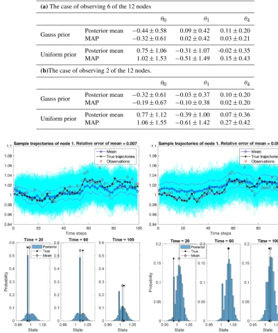
(b)The case of observing 2 of the 12 nodes.
θ0 θ1 θ4
Gauss prior Posterior mean −0.32±0.61 −0.03±0.37 0.10±0.20 MAP −0.19±0.67 −0.10±0.38 0.02±0.20
Uniform prior Posterior mean 0.77±1.12 −0.39±1.00 0.07±0.36 MAP 1.06±1.55 −0.61±1.42 0.27±0.42
Figure 9.The ensemble of sample trajectories of the state at an observed node. Top row: the sample trajectories (in cyan) concentrate around the true trajectory (in black dash-asterisk). The true trajectory is well-estimated by the ensemble mean (in blue dash-diamond) and is mostly enclosed by the 1-standard-deviation band (in magenta dash-dot lines). The relative error of the ensemble mean along the trajectory is 0.7 % and 0.8 %, filtering out 30 % and 20 % of the observation noise, respectively. Bottom row: histograms of samples at three instants of time: t=20,t=60, andt=100. The histograms show that the samples concentrate around the true states.
in the case of Gaussian priors, the peaks of the histogram are close to the true states, even when the histograms form a multi-modal distribution due to the degeneracy of SMC.
We find that the posterior is able to filter out the noise in the observed nodes and reduce the uncertainty in the
pos-Figure 10.The ensemble of sample trajectories of the state at an unobserved node. The ensembles exhibit a large uncertainty in both cases of priors, but the posterior means achieve relative errors of 0.8 % and 3.3 % in the cases of Gaussian and uniform priors, respectively. The 1-standard-deviation band covers the true trajectory at most times. Bottom row: the histogram of samples at three time instants, showing that the samples concentrate around the true states. Particularly, in the case of the Gaussian prior, the peaks of the histogram are close to the true states, even when the histograms form a multi-mode distribution.
terior samples spreads more widely and only slightly reduces the uncertainty.
The coverage probability (CP), the proportion of the states whose 90 % credible intervals contain the true values, is 95 % in the Gaussian prior case and 92 % for the uniform prior in the above simulation. The target probability is 90 %, as in this case 90 % of the true values would be covered by 90 % credible intervals. The values indicate statistically meaningful uncertainty estimates, for example larger uncer-tainty ranges at nodes with higher mean errors. The slight over-dispersiveness, i.e., higher CPs than the target probabil-ities, might be a result of the large uncertainty in the param-eter estimates.
Table 6 shows the means and standard deviations of the relative errors and CPs in state estimation by the posterior mean in 100 independent simulations, averaging over ob-served and unobob-served notes. The relative errors at each time
t are computed by averaging the error of the ensemble mean (relative to the true value) over all the nodes. The relative er-ror of the trajectory is the average over all times along the trajectory. The relative errors are 1.14 % and 2.39 %, respec-tively, for the cases of Gaussian and uniform priors. These numbers are a result of averaging over the observed and
un-observed nodes. Note that the relative errors are similar at different timest=(20,60,100), indicating that the MCMC is able to ameliorate the degeneracy of the SMC to faithfully sample the posterior of the states.
Trajectory t=20 t=60 t=100 CP
Gaussian prior (%) 1.43±0.44 1.38±0.53 1.43±0.51 1.33±0.54 92±6 Uniform prior (%) 2.46±1.28 2.47±1.35 2.49±1.33 2.47±1.34 75±25
5 Discussion
5.1 Observing fewer nodes
We tested the consequences of having sparser observations in space, e.g., observing only 2 out of the 12 nodes. In the Gaussian prior case, in a typical simulation with the same true parameters and observation data as in Sect. 4.2, the rela-tive error in state estimation increases slightly, from 0.7 % to 0.8 % for the observed node and from 0.8 % to 1.1 % for the unobserved node. As a result, the overall error increases. The parameter estimates show small but noticeable changes (see Fig. 11): the posteriors of the parameters have slightly wider support and the posterior means and MAPs exhibit slightly larger errors than those in Sect. 4.2.
We also ran 100 independent simulations to investigate sampling variability in the state and parameter estimates. Table 6b reports the means and standard deviations of the relative errors of the posterior mean trajectory, and CPs for state estimation in these simulations. The Gaussian prior case shows small increases in both the means and the standard de-viations of errors, as well as slightly lower and less robust CPs. This confirms the results quoted above for a typical sim-ulation. The uniform prior case shows almost negligible error and CP increases. Table 5b reports the means and standard deviations of the posterior means and MAP for parameter es-timation in these simulations. Small changes in comparison to the results in Table 5a are found. These small changes are due to the strong regularization that has been introduced to overcome the degeneracy of the likelihood.
5.2 Observing a longer trajectory
When the length N of the trajectory of observation in-creases, the exponent of the regularized posterior Eq. (19), viewed as a function of θ only, tends to its expectation with respect to the ergodic measure of the system, i.e.,
1
NCy1:N(θ, u1:N)
N→∞
−−−−→E[Cy1:N(θ, u1:N)]almost surely. As
a result, the marginal posterior tends to be stable as N
in-creases. This result indicates that an increase in data size has a limited effect on the regularized posterior of parame-ters. This fact is verified by numerical tests withN=1000, in which the marginal posteriors only have a slightly wider support than those in Fig. 7 withN=100.
In general, the number of observations needed for the pos-terior to reach a steady state depends on the dimension of the parameters and the speed of convergence to the ergodic measure of the system. Here we have only three parameters and the SEBM converges to its stationary measure exponen-tially (in fewer than 10 time steps); therefore, N=100 is large enough to make the posterior be close to the steady state.
Figure 11.The case of observing 2 out of the 12 nodes: marginal posteriors ofθ. With the same true parameters and the same observation dataset as in Fig. 7, the marginal posteriors have slightly wider supports.
2016; Lu et al., 2015; Jiang and Harlim, 2018). In a paleo-climate reconstruction context, the number of observations will generally be determined by available observations and the length of the reconstruction period rather than by compu-tational considerations. We leave these further developments of efficient sampling methods for long trajectories as a direc-tion of future research.
5.3 Estimates of the nonlinear function
One goal of parameter estimation is to identify the nonlinear functiongθ (specified in Eq. 2) in the SEBM. The posterior
of the parameters also quantifies the uncertainty in the iden-tification of gθ. Figure 12 shows the nonlinear functiongθ
associated with the true parameters and with the MAPs and posterior means presented in Fig. 7, superposed on an ensem-ble of the nonlinear function evaluated with all the samples. Note that in the Gaussian prior case, the true and estimated functionsgθare close even thoughθ4is estimated with large biases by either the posterior mean or by the MAP. In the uni-form prior case, the posterior mean has a smaller error than the MAP and leads to a better estimate of the nonlinear func-tion. In either case, the large band of the ensemble represents a large uncertainty in the estimates.
For the Gaussian prior, neither the posterior distribution of the equilibrium stateue(for whichgθ(ue)=0) nor of the feedback strength dgθ/du(ue)is substantially changed from the corresponding priors. Both experience only a small re-duction of uncertainty. In contrast, the posterior distributions are narrower than the priors for the uniform prior case – al-though the posterior means and MAPs are both biased.
5.4 Implications for paleoclimate reconstructions
Our analysis shows that assessing the well-posedness of the inverse problem of parameter estimation is a necessary first step for paleoclimate reconstructions making use of physi-cally motivated parametric models. When the problem is ill-posed, a straightforward Bayesian inference will lead to bi-ased and unphysical parameter estimates. We overcome this issue by using regularized posteriors, resulting in parameter estimates in the physically reasonable range with quantified uncertainty. However, it should be kept in mind that this ap-proach relies strongly on high-quality prior distributions.
The ill-posedness of the parameter estimation problem for the model we have considered is of particular interest be-cause the form of the nonlinear functiongθ(u)is not
arbi-trary but is motivated by the physics of the energy budget of the atmosphere. The fact that wide ranges of the parameters
θi are consistent with the “observations” even in this highly
idealized setting indicates that surface temperature observa-tions themselves may not be sufficient to constrain physi-cally important parameters such as albedo, graybody ther-mal emissivity, or air–sea exchange coefficients separately. While state-space modeling approaches allow reconstruction of past surface climate states, it may be the case that the asso-ciated climate forcing may not contain sufficient information to extract the relative contributions of the individual physical processes that produced it. Further research will be neces-sary to understand whether the contribution of, e.g., a single process like graybody thermal emissivity can be reliably es-timated from the observations if regularized posteriors are used to constrain the other parameters ofgθ(u).
con-Figure 12.Top row: the true nonlinear functiongθand its estimators using the posterior mean and MAP, superposed on the ensemble of all estimators using the samples. Bottom row: the distribution of the equilibrium stateue(i.e., the zero of the nonlinear functiongθ(·)) and the distribution of dgθ
du(ue), withθbeing samples of the prior and of the posterior.
cern regarding the parametric form ofg, re-parametrization or nonparametric Bayesian inference can be used to esti-mate the form of the nonlinear functiongbut avoid the ill-posedness of the parameter estimation problem. This is an option if the interest is in the posterior of the climate state and not in the individual contributions of energy sink and source processes.
State-of-the-art observation operators in paleoclimatol-ogy are often nonlinear and contain non-Gaussian elements (Haslett et al., 2006; Tolwinski-Ward et al., 2011). A lo-cally linearized observation model with data coming from the interpolation of proxy data can be used in the modeling framework we have considered, along with the assumption of Gaussian observation noise. Alternatively, it is also pos-sible to first compute offline point-wise reconstructions by inverting the full observation operator, potentially interpo-lating the results in time, and using a Gaussian approxima-tion of the point-wise posterior distribuapproxima-tions as observaapproxima-tions in the SEBM (e.g., Parnell et al., 2016). We anticipate that such simplified observation operators will limit the accuracy of the parameter estimation but that the regularized poste-rior would still be able to distinguish the most likely states and quantify the uncertainty in the estimation. Directly us-ing nonlinear, non-Gaussian observation operators requires a more sophisticated particle filter as optimal filtering is no
longer possible. Such approaches will increase the computa-tional cost and face difficulties in avoiding filter degeneracy.
6 Conclusions and future work
We have investigated the joint state-parameter estimation of a nonlinear stochastic energy balance model (SEBM) mo-tivated by the problem of spatial–temporal paleoclimate re-construction from sparse and noisy data, for which parame-ter estimation is an ill-posed inverse problem. We introduced strongly regularized posteriors to overcome the ill-posedness by restricting the parameters and states to physical ranges and by normalizing the likelihood function. We considered both a uniform prior and a more informative Gaussian prior based on the physical ranges of the parameters. We sam-pled the regularized high-dimensional posteriors by a parti-cle Gibbs with ancestor sampling (PGAS) sampler that com-bines Markov chain Monte Carlo (MCMC) with an optimal particle filter to exploit the forward structure of the SEBM.
leading to slightly larger uncertainties due to less informa-tion. However, due to the need for regularization to over-come ill-posedness, the uncertainty in the posterior of the parameters cannot be eliminated by increasing the number of observations in time. Therefore, we suggest alternative ap-proaches, such as re-parametrization of the nonlinear func-tion according to the climatological distribufunc-tion or nonpara-metric Bayesian inference (see, e.g., Müller and Mitra, 2013; Ghosal and Van der Vaart, 2017), to avoid ill-posedness.
This work shows that it is necessary to assess the well-posedness of the inverse problem of parameter estimation when reconstructing paleoclimate fields with physically mo-tivated parametric stochastic models. In our case, the natural physical formulation of the SEBM is ill-posed. While climate states can be reconstructed, values of individual parameters are not strongly constrained by the observations. Regularized posteriors are a way to overcome the ill-posedness but retain a specific parametric form of the nonlinear function repre-senting the climate forcings.
u(t, ξ )by
udb(t, ξ )=
db
X
i=1
bui(t )φi(ξ ). (A1)
The coefficientsbui are determined by the following weak Galerkin projection of the SEBM Eq. (1):
hudb(t,·), φi = hu0, φi −ν
t Z
0
h∇udb(s,·),∇φids
+
t Z
0
hgθ(udb(s,·)), φids+
t Z
0
hf (s,·), φi, (A2)
whereφis a continuously differentiable compactly supported test function and the integralR0thf (s,·), φiis an Itô integral. For convenience, we write this Galerkin approximate sys-tem in vector notation. Denote
U (t )=
bu1(t ), . . .,budb(t )
T
, (A3)
8(ξ )= φ1(ξ ), . . ., φdb(ξ )
T
, (A4)
udb(t, ξ )=UT(t )8(x)=8T(x)U (t ). (A5) Takingφ=φj,j =1, . . ., dbin Eq. (A2) and using the sym-metry of the inner product, we obtain a stochastic integral equation for the coefficientU (t )∈Rdb:
h8, 8TiU (t )= h8, 8TiU (0)−νh∇8,∇8Ti
t Z
0
U (s)ds+
t Z
0
hgθ(UnT8), 8ids+ t Z
0
hf (s,·), 8i. (A6)
To simplify notation, we denote the mass and stiffness matri-ces by
M0= h8, 8Ti, M1=νh∇8,∇8Ti, (A7) which are symmetric, tri-diagonal, positive definite matrices inRdb×db, and we denote the nonlinear term as
Gθ(U (t )):= hgθ(UT(t )8), 8i. (A8)
The mesh on the sphere and the matricesM0 and M1 are computed with R package INLA (Lindgren and Rue, 2015; Bakka et al., 2018).
A1.2 Representation of the nonlinear term
The parametric nonlinear functional Gθ(U (t )) is
approxi-mated using the finite elements. We approximate each spatial integration over an element triangle inhgθ(UnT8), 8iby the volume of the triangular pyramid whose height is the value of the nonlinear function at the center of the element triangle Tk, i.e.,
Z
gθ(u(t, ξ ))φl(ξ )dξ≈ X
Tk⊂supp(φl)
Area(Tk)
3 gθ
X
i
Ui(t )φi(ξkc) !
, (A10)
whereξkc is the center of the triangleTk. In the discretized
system, we assume that this approximation has a negligible error and take it as our nonlinear functional. In vector nota-tion, it reads
Gθ(U (t ))=ATgθ(AU (t )), (A11)
withAT =
Area(Tk)
3
∈Rdb×de withd
e denoting the num-ber of triangle elements and the matrix A= φi(ξkc)
∈
Rde×db, such that the function gθ(AU (t )) is interpreted as
an element-wise evaluation. For the nonlinear functiongθin
Eq. (2), we can write the above nonlinear term as
Gθ(U (t ))= X
k=0,1,4
θkAT(AU (t ))◦k, (A12)
where◦kdenotes the entry-wise product of the array. A1.3 Representation of the stochastic forcing
Following Lindgren et al. (2011), the stochastic forcing
f (t, ξ )is approximated by its linear finite-element trunca-tion,
f (t, ξ )=
db
X
i=1
(ρ−2M0+M1) F (t ) = σfh8, W (t,·)i, (A15) where the random vector h8, W (t,·)i :=
hφ1, W (t,·)i, . . .,hφdb, W (t,·)i
is Gaussian with mean 0 and covarianceM0. Solving Eq. (A15) yields
F (t ) ∼N0, σf2Mρ−1M0M−ρ1
, (A16)
whereMρ:=(ρ−2M0+M1).
A1.4 Semi-backward Euler time integration
Equation (A9) is integrated in time by a semi-backward Euler scheme:
M1tUn+1=M0Un+1t Gθ(Un)+
√
1tM0Fn, (A17)
whereUnis the approximation ofU (tn)withtn=n1t, and
{Fn} is a sequence of iid random vectors with distribution
N 0, σf2M−ρ1M0M−ρ1, with the matrixM1t denoting
M1t:=M0+1tM1. (A18)
A1.5 Efficient generation of the Gaussian field
It follows from Eq. (A15) thatM0Fnis Gaussian with mean
zero and covariance M0M−ρ1M0M−ρ1M0. Note that while Mρ is a sparse matrix, its inverse matrix M−ρ1 is not. To
efficiently use the sparseness of Mρ, following Lindgren
et al. (2011), we approximateM0byMb0:=diag(hφi,1i)and
compute the noise M0Fn byC−1N(0, Id), whereCis the
Cholesky factorization of the inverse of the covariance ma-trix (called the precision mama-trix)Mb
−1 0 MκMb
−1 0 MκMb
−1 0 .The precision matrix is a sparse representation of the inverse of the covariance. Therefore, the matrixCis also sparse and the noise sequence can be efficiently generated.
In summary, we can write the discretized SEBM in the form
Un+1=µθ(Un)+Wn, (A19)
where the deterministic functionµθ(·)is given by µθ(Un)=M−1t1M0Un+
X
k=0,1,4
θkGθ,k(Un), (A20)
b 1:N 1:N
m=1
n U1:n 1:N
withPM
m=1wmn =1. These weighted samples are drawn
se-quentially by importance sampling based on the recurrent formation
p(u1:n|y1:n)=p(u1:n−1|y1:n−1)
p (yn|un) p(un|un−1)
p(yn|y1:n−1)
. (A23)
More precisely, suppose that at time n, we have weighted samples {U1m:n−1, wmn−1}M
m=1. One first draws a sampleUnm
from an easy-to-sample importance densityq(un|yn, Unm−1) that approximates the “incremental density” which is pro-portional top (yn|un) p(un|Unm−1)for eachm=1, . . ., Mand computes incremental weights
αnm=p(U
m
n |Unm−1)p(yn|Unm) q(Um
n|yn, Unm−1)
, (A24)
which account for the discrepancy between the two densities. One then assigns normalized weights{wnm ∝wnm−1αnm}M
m=1 to the concatenated sample trajectories{U1m:n}M
m=1.
A clear drawback of the above procedure is that all but one of the weights {wnm} will become close to zero as the number of iterations increases, due to the multiplica-tion and normalizamultiplica-tion operamultiplica-tions. To avoid this, one re-places the unevenly weighted samples{(Unm−1, wnm−1)}with uniformly weighted samples from the approximate density b
pθ(un−1|y1:N−1). This is the well-known resampling tech-nique. In summary, the above operations are carried out as follows:
i. draw random indices{Amn−1}M
m=1 according to the dis-crete probability distribution F(·|w1n:−M1) on the set {1, . . ., M}, which is defined as
F(An−1=k|w1n:−M1)=wnk−1,fork=1, . . ., M; (A25)
ii. for eachm, draw a sampleUnm from q(un|yn, U Amn−1 n−1 ) and setU1m:n:=(UA
m n−1
Doucet and Johansen, 2011) and is summarized in Algo-rithm 1.
A2.1 Optimal importance sampling
Note that the conditional transition density of the states
pθ(un+1|un) in Eq. (7) is Gaussian and the observation model in Eq. (8) is linear and Gaussian. These facts allow for a Gaussian optimal importance density q(un|yn, Unm−1)
that is proportional to p (yn|un) p(un|Unm−1) for each m= 1, . . ., M:
q(un|yn, Unm−1)∼N(µmn,6), (A27)
with the meanµmn and the covariance6given by
µmn =µ(Unm−1)+RHTQ−1(yn−Hµ(Unm−1)), (A28)
6=R−RHTQ+HRHT
−1
HR. (A29)
A2.2 Drawbacks of SMC
While the resampling technique preventswnmfrom being de-generate at each current timen, SMC algorithms suffer from the degeneracy (or particle depletion) problem: the marginal distributionp(ub n|(y1:N))becomes concentrated on a single
particle asN−nincreases because each resampling step re-duces the number of distinct particles ofun. As a result, the estimate of the joint density p(u1:N|y1:N)of the trajectory
deteriorates as timeN increases. A3 Particle Gibbs and PGAS
The framework of particle MCMC introduced in Andrieu et al. (2010) is a systematic combination of SMC and MCMC methods, exploiting the strengths of both techniques. Among the various particle MCMC methods, we focus on the parti-cle Gibbs sampler (PG) that uses a novel conditional SMC update (Andrieu et al., 2010), as well as its variant, the parti-cle Gibbs with ancestor sampling(PGAS) sampler (Lindsten et al., 2014), because they are best fit for sampling our joint parameter and state posterior.
The PG and PGAS samplers use a conditional SMC up-date step to realize the transition between two steps of the Markov chain while ensuring that the target distribution will be the stationary distribution of the Markov chain. The basic procedure of a PG sampler is as follows.
That is, in the SMC algorithm, the Mth particle is required to move along the reference trajectory by settingUnM=Un(l). Draw other samples from the importance density, and normalize the weights and resample all the particles as usual. This leads to weighted samples{U1m:N, wNm}M
m=1withU
M
1:N= U1:N(l); and
c. drawU1:N(l+1)from the above weighted samples.
– Return the Markov chain{θ (l), U1:N(l)}Ll=1.
The conditional SMC algorithm is the core of PG sam-plers. It retains the reference path throughout the resam-pling steps by deterministically settingU1M:N=U1:N(l) and
AMn =Mfor allnwhile sampling the remainingM−1 par-ticles according to a standard SMC algorithm. The reference path interacts with the other paths by contributing a weight
wMn . This is the key to ensuring that the PG Markov chain converges to the target distribution. A potential risk of the PG sampler is that it yields a poorly mixed Markov chain, because the reference trajectory tends to dominate the SMC ensemble trajectories.
The PGAS sampler increases the mixing of the chain by connecting the reference path to the history of other parti-cles by assigning an ancestor to the reference particle at each time. This is accomplished by drawing a sample for the an-cestor indexAMn−1of the reference particle, which is referred to asancestor sampling. The distribution of the indexAMn−1
is determined by the likelihood of connectingUn(l) to the particles{Unm−1}M
m=1, in other words, according to weights eα
m
n−1|n=w m
n−1pθ (l+1)(Un(l)|U
m
n−1)p(yn|Un(l)),
e wnm−1|n=
eα m n−1 PM
k=1eα k n−1
. (A30)
The above weight eαnm−1|n can be seen as a posterior probability, where the importance weight wnm−1 is the prior probability of the particle Unm−1 and the product
pθ (l+1)(Un(l)|Unm−1)p(yn|Un(l))is the likelihood thatUn(l) originates fromUnm−1conditional on observationyn. In short,
the PGAS sampler assigns the reference particleUn(l)an
an-cestorAMn−1 that is drawn from the distribution F(AMn−1=
k| e
wn1:−M1|n)= e wnk−1|n.
Disclaimer. Any opinions, findings, and conclusions or recommen-dations expressed in this material are those of the author(s) and do not necessarily reflect the views of the National Science Founda-tion.
Acknowledgements. The authors thank Colin Grudzien and the other reviewer for helpful comments. This research started in a working group supported by the Statistical and Applied Mathematical Sciences Institute (SAMSI). Fei Lu thanks Pe-ter Jan van Leeuwen, Kayo Ide, Mauro Maggioni, Xuemin Tu, and Wenjun Ma for helpful discussions. Fei Lu is supported by the Na-tional Science Foundation under grant DMS-1821211. Nils Weitzel thanks Andreas Hense and Douglas Nychka for inspiring discus-sions. Nils Weitzel was supported by the German Federal Ministry of Education and Research (BMBF) through the Palmod project (FKZ: 01LP1509D). Nils Weitzel thanks the German Research Foundation (code RE3994-2/1) for funding. Adam H. Monahan ac-knowledges support from the Natural Sciences and Engineering Re-search Council of Canada (NSERC), and thanks SAMSI for hosting him in the autumn of 2017.
Financial support. This research has been supported by the Na-tional Science Foundation, USA (grant no. DMS-1821211), the German Federal Ministry of Education and Research (BMBF) (grant no. FKZ: 01LP1509D), the German Research Foundation (grant no. RE3994-2/1), and the Natural Sciences and Engineering Research Council of Canada (NSERC).
Review statement. This paper was edited by Stefano Pierini and re-viewed by Colin Grudzien and one anonymous referee.
References
Alberty, J., Carstensen, C., and Funken, S. A.: Remarks around 50 lines of Matlab: short finite element implementation, Numer. Al-gorithms, 20, 117–137, 1999.
Andrieu, C., Doucet, A., and Holenstein, R.: Particle Markov chain Monte Carlo methods, J. R. Stat. Soc. B, 72, 269–342, 2010. Annan, J., Hargreaves, J., Edwards, N., and Marsh, R.: Parameter
estimation in an intermediate complexity Earth System Model using an ensemble Kalman filter, Ocean Model., 8, 135–154, 2005.
Markov Models (Springer Series in Statistics), Springer-Verlag, New York, NY, USA, 2005.
Carrassi, A., Bocquet, M., Bertino, L., and Evensen, G.: Data assimilation in the geosciences: An overview of methods, issues, and perspectives, WIRES Clim. Change, 9, e535, https://doi.org/10.1002/wcc.535, 2018.
Chekroun, M. D. and Kondrashov, D.: Data-adaptive harmonic spectra and multilayer Stuart-Landau models, Chaos, 27, 093110, https://doi.org/10.1063/1.4989400, 2017.
Chorin, A. J. and Tu, X.: Implicit sampling for particle filters, P. Natl. Acad. Sci. USA, 106, 17249–17254, 2009.
Chorin, A. J. and Lu, F.: Discrete approach to stochastic parametrization and dimension reduction in nonlinear dynamics, P. Natl. Acad. Sci. USA, 112, 9804–9809, 2015.
Chorin, A. J., Lu, F., Miller, R. M., Morzfeld, M., and Tu, X.: Sam-pling, feasibility, and priors in data assimilation, Discrete Contin. Dyn. Syst. A, 36, 4227–4246, 2016.
Cowles, M. K. and Carlin, B. P.: Markov chain Monte Carlo con-vergence diagnostics: a comparative review, J. Am. Stat. Assoc., 91, 883–904, 1996.
Cui, T., Marzouk, Y. M., and Willcox, K. E.: Data-driven model reduction for the Bayesian solution of inverse problems, Int. J. Numer. Methods Fluids, 102, 966–990, 2015.
Doucet, A. and Johansen, A. M.: A tutorial on particle filtering and smoothing: fifteen years later, in: Oxford Handbook of Nonlinear Filtering, 656–704, 2011.
Fang, M. and Li, X.: Paleoclimate Data Assimilation: Its Motiva-tion, Progress and Prospects, Sci. China Earth Sci., 59, 1817– 1826, https://doi.org/10.1007/s11430-015-5432-6, 2016. Fanning, A. F. and Weaver, A. J.: An atmospheric energy-moisture
balance model: Climatology, interpentadal climate change, and coupling to an ocean general circulation model, J. Geophys. Res.-Atmos., 101, 15111–15128, 1996.
Farchi, A. and Bocquet, M.: Review article: Comparison of local particle filters and new implementations, Nonlin. Processes Geo-phys., 25, 765–807, https://doi.org/10.5194/npg-25-765-2018, 2018.
Ghosal, S. and Van der Vaart, A.: Fundamentals of nonparametric Bayesian inference, vol. 44, Cambridge University Press, 2017. Goosse, H., Crespin, E., de Montety, A., Mann, M. E., Renssen,
H., and Timmermann, A.: Reconstructing Surface Tempera-ture Changes over the Past 600 Years Using Climate Model Simulations with Data Assimilation, J. Geophys. Res., 115, https://doi.org/10.1029/2009JD012737, 2010.