Mathematical and Software Engineering, Vol. 3, No. 1 (2017), 156-163 Varεpsilon Ltd, varepsilon.com
Optimization of CCIR Pathloss Model Using
Terrain Roughness Parameter
Nathaniel Chimaobi Nnadi
*, Ifeanyi Chima Nnadi, and
Charles Chukwuemeka Nnadi
*Corresponding Author: [email protected]
Department of Electrical/Electronic Engineering, Imo State Polytechnic, Umuagwo, Owerri, Nigeria
Abstract
In this paper, optimizing CCIR pathloss model using terrain roughness parameter is presented. The study is based on field measurement of received signal strength and elevation profile data obtained in a suburban area of Uyo for 800 MHz GSM network. Particularly, in this paper, the mean elevation and the standard deviation of elevation are used separately to minimize the error using least square method. The results show that the untuned CCIR model has a RMSE of 28.8 dB and prediction accuracy of 77.4 %. On the other hand, both the pathloss predicted by the mean elevation tuned CCIR model and the pathloss predicted by the standard deviation of elevation tuned CCIR model have the same RME of 3.9 dB and prediction accuracy of 97.6 %. The terrain roughness correction factors are the same value (that is, = Š= 28.50882771). The RMSE of 3.9dB shows that the terrain roughness parameter-based tuning approach can effectively be used to minimize the prediction error of the CCIR model within the acceptable value which is about 7dB to 10 dB for suburban and rural areas.
Keywords: Pathloss Model, Least Square Error method, Terrain Roughness, Propagation Model Optimization, Elevation Profile, Pathloss Model Optimization
1. Introduction
Empirical pathloss models are usually used to predict the expected pathloss that wireless signals will experience in a given area [1-5]. Accordingly, appropriate pathloss model is usually used required during wireless network planning stage. In practice, pathloss prediction performance of different pathloss models is first evaluated and the model with the best prediction performance is selected and further optimized to improve on its pathloss prediction efficiency.
very simple but in some cases it fails to reduce the prediction error to a value that is within the acceptable range. Above all, if the RMSE for a pathloss prediction model is above 6 dB, then its prediction is considered unacceptable. In view of this limitation, other approaches to pathloss model tuning is required.
In this paper, two terrain parameter-based tuning approaches are presented, one based on the mean terrain elevation and the second based on the standard deviation of the terrain. The prediction performance of the two approaches are compared to that of the RMSE-based tuning approach.
2. Theoretical Background
2.1. CCIR Pathloss Model
In order to account for varying degrees of urbanization, the CCIR (Comit´e Inter-national des Radio-Communication, now ITU-R) developed an empirical model for the pathloss as follows [14-17]:
() = + ∗ log() − (1) where A and B are defined in the Okumura-Hata model with (ℎ) being the medium or small city value.
= 69.55 + 26.16 ∗ log(#) − 13.82 ∗ log(ℎ&) − (ℎ) (2) = 44.9 − 6.55 ∗ log(ℎ&) (3) (ℎ) = (1.1 ∗ log(#) − 0.7+ ∗ ℎ − (1.56 ∗ log(#) − 0.8+ (4)
Eq 4 is for small city, medium city, open area, rural area and suburban area. The parameter E accounts for the degree of urbanization and is given by
E = 30 − 25log() (5) Where PB is the % of area covered by buildings
where E = 0 when the area is covered by approximately 16% buildings.
For Urban Area PB ≥ 16% and hence , E is set to 0 for urban area. For Sub-Urban Area PB < 16% (typical PB =8%) .
For Rural Area PB < 16% (typical PB =3%) .
Where
• f is the centre frequency f in MHz
• d is the link distance in km
• (ℎ) is an antenna height-gain correction factor that depends upon the environment
• 150 MHz≤ f≤ 1000MHz
• 30m ≤ℎ& ≤ 200m
• 1m≤ ℎ≤ 10 m
• 1 km ≤ d ≤ 20km
2.2. The Terrain Roughness-Based Pathloss Model Tuning
Approaches
literatures, the standard deviation of the terrain elevation profile is used to denote the terrain roughness index. In this paper, two terrain parameters are used, namely, the mean elevation and the standard deviation of the elevation. Each of the two terrain parameters are used to optimize the pathloss prediction of CCIR model. Let the mean elevation be denoted as M and the mean elevation-based terrain roughness correction factor be denoted as C. where,
C. = K.(M) (6)
K. is the tuning coefficient for the mean elevation-based terrain roughness correction factor
Let the standard deviation of elevation be denoted as Š and the standard deviation of elevation-based terrain roughness correction factor be denoted as Š where,
CŠ = KŠ (Š ) (7)
KŠ is the tuning coefficient for the standard deviation of elevation-based terrain roughness correction factor.
2.3. Field Data Collection and Processing
Samsung I9500 Galaxy S4 mobile phone was used to measure the Received Signal Strength (RSS) from the GSM network. Particularly, the Samsung I9500 Galaxy S4 has CellMapper and MyGPS Coordinates Android applications installed. The CellMapper enables the mobile phone to read and display advanced GSM/CDMA/UMTS/LTE current and neighboring cells’ low level data and can also record and export the data as CSV file. Among the data captured by CellMapper are the current and neighboring cells Received Signal Strength (RSS) in dB, the current cells CID, LAC. MyGPS Coordinates is an android application that gives the latitude and longitude of the current location of the mobile phone in both decimal format and sexagesimal (degrees/minutes/seconds) format. The RSS along with the longitude and latitude are reads at each measurement point. In addition, the GSM base station was located and its longitude and latitude are recorded. After the measurements, haversine formula was used along with the longitude and latitude of each of the measurement points and the longitude and latitude of the mast location to determine the distance between the mast and each of the measurement points [18,19]. The Received Signal Strength (RSS) is converted to the measured pathloss (PLm) by using the link budget formula:
(01) = PBTS + GBTS + GMS – LFC – LAB – LCF – RSS(dBm) (8) where
PL4(56) is the measured pathloss for each measurement location at a distance d( km) RSS is the mean Received Signal Strength (RSS) in dBm = the measured received
signal strength.
PBTS = Transmitter Power (dBm), GBTS = Transmitter Antenna Gain (dBi), GMS = receiver antenna gain (dBi), LFC = feeder cable and connector loss (dB), LAB = Antenna Body Loss (dB) and LCF = Combiner And Filter Loss (dB).
The values of these parameters are given as [13] as: PBTS = 40 W = 46 dBm, GBTS = 18.15 dBi, GMS = 0 dBi, LFC = 3 dB, LAB = 3 dB, LCF = 4.7 dB. Hence,
(01) = 53.5 (dBm) .– RSS(dBm) (9)
i) The Root Mean Square Error (RMSE) is calculated as follows:
MSE = DE W FG∑O T FO T I(JKLMNJ0)(O)− (PNJ0OQRJ0)(O) ISUV (10)
ii) Then, the Prediction Accuracy (PA, %) based on mean absolute percentage deviation (MAPD) or Mean Absolute Percentage Error (MAPE) is calculated as follows:
XY = Z1 −F [∑ \I]^(_`abcd`e)(f)g]^(hd`efij`e)(f) I
]^(_`abcd`e)(f) \
OTF
OT kl * 100% (11)
3. Results and Discussions
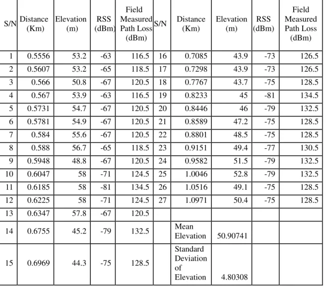
The field measured distance, elevation, received signal strength (RSSI) and pathloss (PLm) are given in Table 1. The measured pathloss (PLm) is obtained by using the link budget equation:
(01) = 53.5 (dBm) – RSS(dBm). The distance is obtained by applying the longitude and latitude of each of the measurement points in the Haversine equation with the longitude 1 and latitude 1 being that of the GSM base station while longitude 2 and latitude 2 is for the measurement point.
Table 1 The Field Measured Distance, Elevation, Received Signal Strength (RSS) and Field Measured Path Loss (PLm)
S/N Distance (Km)
Elevation (m)
RSS (dBm)
Field Measured Path Loss (dBm)
S/N Distance (Km)
Elevation (m)
RSS (dBm)
Field Measured Path Loss (dBm)
1 0.5556 53.2 -63 116.5 16 0.7085 43.9 -73 126.5
2 0.5607 53.2 -65 118.5 17 0.7298 43.9 -73 126.5
3 0.566 50.8 -67 120.5 18 0.7767 43.7 -75 128.5
4 0.567 53.9 -63 116.5 19 0.8233 45 -81 134.5
5 0.5731 54.7 -67 120.5 20 0.8446 46 -79 132.5
6 0.5781 54.9 -67 120.5 21 0.8589 47.2 -75 128.5
7 0.584 55.6 -67 120.5 22 0.8801 48.5 -75 128.5
8 0.588 56.7 -65 118.5 23 0.9151 49.4 -77 130.5
9 0.5948 48.8 -67 120.5 24 0.9582 51.5 -79 132.5
10 0.6047 58 -71 124.5 25 1.0046 52.8 -79 132.5
11 0.6185 58 -81 134.5 26 1.0516 49.1 -75 128.5
12 0.6225 58 -71 124.5 27 1.0971 50.4 -75 128.5
13 0.6347 57.8 -67 120.5
14 0.6755 45.2 -79 132.5
Mean
Elevation 50.90741
15 0.6969 44.3 -75 128.5
Standard Deviation of
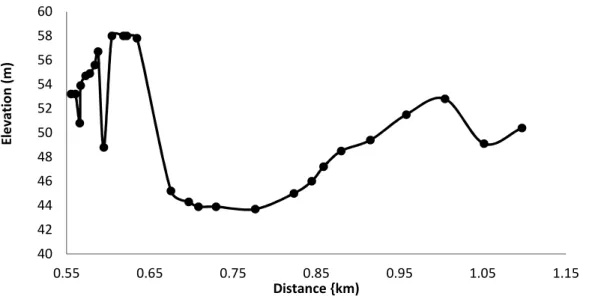
Figure 1 The Elevation Profile of the Terrain
Table 1 also shows the mean elevation and the standard deviation of the elevation of the measurement points. The CCIR model is optimized using the mean elevation and then using the standard deviation of the elevation of the measurement points. The value of m. and also the value of mŠ that minimizes the sum of square error are determined using Microsoft Excel solver least square error optimization tool. The results obtained from the Microsoft Excel solver are m. = 0.560013349 and mŠ = 5.935530824. Therefore, with mean elevation, M =50.90741, m.= 0.560013349, hence:
. = m.(M) = 28.50882771 (12) Also, with standard deviation of elevation (Š) = 4.80308, mŠ= 5.935530824, hence:
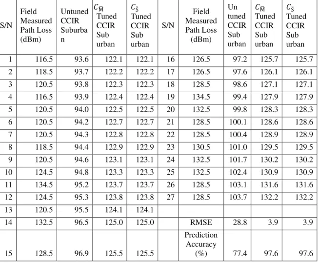
CŠ = KŠnŠo = 28.50882771 (13) Table 2 shows the field measure pathloss and the pathloss predicted by the untuned CCIR model, the pathloss predicted by the mean elevation tuned CCIR model and the pathloss predicted by the standard deviation of elevation tuned CCIR model. Also, the table shows that the untuned CCIR model has a RMSE of 28.8 dB and prediction accuracy of 77.4 %. On the other hand, both the pathloss predicted by the mean elevation tuned CCIR model and the pathloss predicted by the standard deviation of elevation tuned CCIR model have the same RME of 3.9 dB and prediction accuracy of 97.6 %. The terrain roughness correction factors are the same value (that is, . = Š = 28.50882771). The RMSE of 3.9dB shows that the terrain roughness parameter-based tuning approach can effectively be used to minimize the prediction error of the CCIR model within the acceptable value which is about 7dB to 10 dB for suburban and rural areas.
40 42 44 46 48 50 52 54 56 58 60
0.55 0.65 0.75 0.85 0.95 1.05 1.15
E
le
v
a
ti
o
n
(
m
)
Table 2 The field measure pathloss and the pathloss predicted by the untuned and the tuned CCIR models
S/N Field Measured Path Loss (dBm) Untuned CCIR Suburba n . Tuned CCIR Sub urban Š Tuned CCIR Sub urban S/N Field Measured Path Loss (dBm) Un tuned CCIR Sub urban . Tuned CCIR Sub urban Š Tuned CCIR Sub urban
1 116.5 93.6 122.1 122.1 16 126.5 97.2 125.7 125.7
2 118.5 93.7 122.2 122.2 17 126.5 97.6 126.1 126.1
3 120.5 93.8 122.3 122.3 18 128.5 98.6 127.1 127.1
4 116.5 93.9 122.4 122.4 19 134.5 99.4 127.9 127.9
5 120.5 94.0 122.5 122.5 20 132.5 99.8 128.3 128.3
6 120.5 94.2 122.7 122.7 21 128.5 100.1 128.6 128.6
7 120.5 94.3 122.8 122.8 22 128.5 100.4 128.9 128.9
8 118.5 94.4 122.9 122.9 23 130.5 101.0 129.5 129.5
9 120.5 94.6 123.1 123.1 24 132.5 101.7 130.2 130.2
10 124.5 94.8 123.3 123.3 25 132.5 102.4 130.9 130.9
11 134.5 95.2 123.7 123.7 26 128.5 103.1 131.6 131.6
12 124.5 95.3 123.8 123.8 27 128.5 103.7 132.2 132.2
13 120.5 95.5 124.1 124.1
14 132.5 96.5 125.0 125.0 RMSE 28.8 3.9 3.9
15 128.5 96.9 125.5 125.5
Prediction Accuracy
(%) 77.4 97.6 97.6
Figure 2 The field measure pathloss and the pathloss predicted by the untuned and the tuned CCIR models
90 95 100 105 110 115 120 125 130 135 140
0.5 0.6 0.7 0.8 0.9 1 1.1
P a th lo ss ( d B ) Distnace (km)
Field Measured Path Loss (dBm) Untuned CCIR Suburban
4. Conclusion
In this paper, a CCIR pathloss model tuning approach based on terrain roughness parameter is presented. The study is based on empirical field measurement in a suburban area for a GSM network in the 800 MHz frequency band. The mean elevation and the standard deviation of elevation are used separately in this paper to minimize the error using least square method. The results show that the two approach gave the same correction factor for CCIR propagation model and hence, the same RMSE and prediction accuracy. Also, both approach reduced the CCIR model prediction error within the acceptable 7 dB for suburban and rural areas.
References
[1] Popoola, S. I., & Oseni, O. F. (2014) Empirical Path Loss Models for GSM Network Deployment in Makurdi, Nigeria. International Refereed Journal of Engineering and Science, 3(6), 85-94.
[2] Phillips, C., Sicker, D., & Grunwald, D. (2013) A survey of wireless path loss prediction and coverage mapping methods. IEEE Communications Surveys & Tutorials, 15(1), 255-270.
[3] Mardeni, R., Siva Priya, T. (2010) Optimised COST-231 Hata models for WiMAX path loss prediction in suburban and open urban environments. Modern Applied Science, 4(9), 75-89.
[4] Milanović, J., Rimac-Drlje, S., & Majerski, I. (2010) Mehanizmi prostiranja radio vala i empirijski modeli za fiksne radijske pristupne sustave. Tehnički vjesnik, 17(1), 43-53.
[5] Abhayawardhana, V. S., Wassell, I. J., Crosby, D., Sellars, M. P., & Brown, M. G. (2005) Comparison of empirical propagation path loss models for fixed wireless access systems. In 2005 IEEE 61st Vehicular Technology Conference (Vol. 1, pp. 73-77). IEEE.
[6] Aremu, O. A., Taiwo, O. A., Makinde, O. S., & Adeniji, J. A. (2016) Experimental Study of Variation of Path Loss with Respect to Heights at GSM Frequency Band, International Journal of Scientific Research in Science, Engineering and Technology (ijsrset.com), 2(3), 347-351.
[7] Udofia, K.M., Friday, N., & Jimoh, A. J. (2016) Okumura-Hata Propagation Model Tuning Through Composite Function of Prediction Residual. Mathematical and Software Engineering, 2(2), 93-104.
[8] Rath, H. K., Verma, S., Simha, A., & Karandikar, A. (2016) Path Loss model for Indian terrain-empirical approach. In Communication (NCC), 2016 Twenty Second National Conference on (pp. 1-6). IEEE.
[9] Faruk, N., Ayeni, A. A., Adediran, Y. A., & Surajudeen–Bakinde, N. T. (2014) Improved path–loss model for predicting TV coverage for secondary access. International Journal of Wireless and Mobile Computing, 7(6), 565-576. [10] Alshaalan, F., Alshebeili, S., & Adinoyi, A. (2010). On the performance of mobile
[11] Joseph, I., & Konyeha, C. C. (2013) Urban Area Path loss Propagation Prediction and Optimisation Using Hata Model at 800MHz. IOSR Journal of Applied Physics (IOSR-JAP), 3, 8-18.
[12] Nisirat, M. A., Ismail, M., Nissirat, L., & Alkhawaldeh, S. (2012). Linear Regression Route Roughness Parameter to Correct Hata Path Loss Prediction Formula for 1800 MHz. In Progress in Electromagnetics Research Symposium, PIERS 2012 Kuala Lumpur. 1429-1431.
[13] Nadir, Z., & Ahmad, M. I. (2010) Pathloss Determination Using Okumura-Hata Model And Cubic Regression for Missing Data for Oman. In Proceedings of the International MultiConference of Engineering and Computer scientist 2010 (Vol. 2).
[14] Al Mahmud, M.R., Shabbir, Z. (2009) Analysis and planning microwave link to established efficient wireless communications, Thesis, Blekinge Institute of Technology.
[15] Debus, W. (2006) R.F. Path-loss and Transmission distance calculations. Axon, LLC, Technical memorandum.
[16] Negi, A. (2006) Analysis of Relay-based Cellular Systems, Dissertation, Portland State University.
[17] Muhammad, J. (2007) Artificial neural networks for location estimation and co-channel interference suppression in cellular networks, Thesis, University of Stirling.
[18] Mwemezi, J. J., & Huang, Y. (2011) Optimal facility location on spherical surfaces: algorithm and application. New York Science Journal, 4(7), 21-28.
[19] Bullock, R. (2007) Great circle distances and bearings between two locations. MDT.