Vol 60, No 4 (2017)

(1)

TECHNICAL UNIVERSITY OF CLUJ-NAPOCA

ACTA TECHNICA NAPOCENSIS

Series: Applied Mathematics, Mechanics, and Engineering Vol. 60, Issue IV, November, 2017

STUDY OF THE INFLUENCE OF GEOMETRIC PARAMETERS ON THE

DISPLACEMENT OF PISTON AND COMPRESSION RATIO FOR A

VARIABLE COMPRESSION RATIO MECHANISM

Bogdan MĂNESCU, Ionuț DRAGOMIR, Nicolae-Doru STĂNESCU, Nicolae PANDREA

Abstract: A variable compression ratio mechanism is presented and the constrained relations between different parameters are established. The study is performed in two ways: by geometrical and multibody approaches. Based on the formulae deduced in this study, the authors determine the extreme positions of the piston and the compression ratio for certain geometric parameters. The variations of extreme positions and compression ratio depending on the dimensions’ variations of the elements are presented in graphical mode and the conclusions are highlighted. A special attention is paid to the tiller’s curve of a specific point.

Key words: variable compression ratio mechanism, extreme positions, compression ratio, lever’s curve, multibody.

1. INTRODUCTION

Freudenstein and Maki [1] synthesize the constructive solutions of the mechanism of an engine with variable compression ratio with six elements and seven joints, and with eight elements and ten joints. Numerous patens were brevetted in this field [2]. For a spark engine the compression ratio is limited by the materials used in its construction and the phenomenon of knocking. The maximum value of the compression ratio is 13:1, usually being limited to 10:1. The prevention of knocking is made with the aid of the swirl phenomenon that creates a circular motion of the fuel in the combustion chamber in order to homogenize it. The usual methods for the obtaining of the variable compression ratio are:

– articulated engine’s block. Such a method was used by Hara et al. [3], Clenci [4] obtaining a variation of the compression ratio from 8.5:1 to 12.5:1. Another solution is given by SAAB company [5], varying the compression ratio from 8:1 to 14:1;

– modification of the volume of the combustion chamber by adding a supplementary volume. The solution was

adopted by Ford [6] using a small piston acted by a cam;

– modification of the piston’s geometry used by Daimler-Benz and developed by University of Michigan [7];

– tiller eccentrically assembled by inserting an eccentric between the tiller and the crankshaft. Another construction is based on the use of a worm gear, the compression ratio varying between 8.5:1 and 14:1 [8];

– eccentric crankshaft presented by FEV in 2007 and obtaining a compression ratio between 8:1 and 16:1 [9];

– a combination of the crank-shaft and gear mechanisms, used by PSA Group and leading the compression ratio between 6:1 and 15:1 [10];

– additional different kinematic joints of the crank-shaft mechanism. This solution is used by Nissan for compression ratios between 8:1 and 14:1 [11].

Some aspects concerning the transitory vibration for a variable compression ratio mechanism was studied by the authors in [12].

(2)

ϕ₃

4

ϕ

2

ϕ

1

ϕ

O C

A

C E

Y

X B

1

2

C

3

C

4

C

5

C D e

d

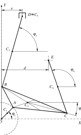
Fig. 1. The mechanism.

2. THE MECHANISM

The mechanism is presented in Fig. 1. It contains the shaft OC, intermediate triangular element ABC, crank BD, piston situated at the point D, and the control element CE. The crankshaft rotates uniformly with an angular velocity ω. The control element has a determined motion which is considered to be known, YE =YE

( )

t . The system has five

elements and, that is, it has maximum 15 possible degrees of freedom. The position of the mechanism is described by the positions of the centers of weight of the five elements,

i

C X ,

i

C

Y , and the rotational angles of them ϕ_i,

5 , 1 =

i . The displacement between the Y-axis and the direction of motion of the piston is equal to e; usually e has small values and in the most cases e = 0. The coordinate X_E, which is a constant of the mechanism is denoted by d.

3. GEOMETRIC APPROACH

Further on, we make the following notations:

– OXY – the fixed reference frame

– Ci, i =1 ,5 – centers of mass of the elements, assumed to be homogeneous;

– C₁x₁y₁ – mobile reference system attached to the element OA and having the x₁-axis along the line OA and orientated from point C₁

to point A;

– C₂x₂y₂ – mobile reference system attached to the triangular element ABC with the x₂-axis situated along the line C₂C and orientated from point C₂ to point C;

– C₃x₃y₃ – mobile reference frame attached

to the element BD and having the x₃-axis along the line BD and orientated from point

3

C to point D;

– C₄x₄y₄ – mobile reference frame attached to the element CE, with the x₄-axis along the line CE and orientated from point C₄ to point

E;

– C₅x₅y₅ – mobile reference system attached to the piston (element 5) and having the axes parallel to the axes of the fixed reference system;

– ϕ_i, i =1 ,5 – the rotational angles of the mobile reference systems. One may observe that always

0

5 =

ϕ ; (1)

–

[ ]

Ai , i =1 ,5 – the rotation matrices,

[ ]



  

 

ϕ ϕ

ϕ − ϕ =

i i

i

cos sin

sin cos

A ; (2)

– XP, YP – the coordinates of a generic point P relative to the fixed system of coordinates;

– ( )i P x , ( )i

P

y – the coordinates of the generic point P relative to the mobile system of coordinates Cixiyi, i =1 ,5;

(3)

– θ – the angle BC₂C.

The coordinates of the point A are

1

cosϕ

= OA

XA , YA = OAsinϕ1. (3)

The coordinates of the point E are

d

XE = , YE = h, (4)

where the dimension h are considered to be known at each moment of time.

Point C is obtained as the intersection between the circle with center at the point A

and radius AC, and the circle with the center at the point E and radius CE, that is, the coordinates of the point C are the solutions of the system

(

)

2

(

)

2

(

)

2

AC Y

Y X

X − _A + − _A = ,

(

)

2

(

)

2

(

)

2

CE Y

Y X

X − _E + − _E = . (5)

It results 1 1 1 2 2 e e d e e

X_C = − + + , Y_C = aX_C +b, ₍₆₎

where

( )

(

)

, 2 2 2 2 2 2 2 2 E A E

A X Y Y

X CE CA c + − + − + − = (7) A E A E Y Y X X a − − −

= , ₍₈₎

A E Y Y c b −

= , ₍₉₎

2 1 1 a

e = + , (10)

A A X aY ab

e₂ = − − , (11)

( )

2 ₂

(

)

2

1 CA XA b YA

d = − − − . (12)

Similarly, point B is the intersection between the circle with the center at the point

A and the radius equal to AB, and the circle with the center at the point C and the radius equal to BC, that is, the coordinates of the point B are the solution of the system

(

)

2

(

)

2

(

)

2

AB Y

Y X

X − _A + − _A = ,

(

)

2

(

)

2

(

)

2

BC Y

Y X

X − C + − C = .

(13) We obtain 1 1 1 2 2 e e d e e XB + + −

= , YB = aXC +b, (14)

in which the parameters e₁, e₂, a, b, and c

are given by

(

)

(

)

, 2 2 2 2 2 2 2 2 C A C

A X Y Y

X BC AB c + − + − + − = (15) A C A C Y Y X X a − − −

= , ₍₁₆₎

A C Y Y c b −

= , ₍₁₇₎

2 1 1 a

e = + , (18)

A A X aY ab

e2 = − − , (19)

(

)

2 ₂

(

)

2

1 AB XA b YA

d = − − − . (20)

Point D is situated at the intersection of the circle with the center at the point B and radius

BD, and the vertical line of equation X_D = e. We obtain the values

e X_D = ,

(

)

2

(

)

2

B D B

D Y BD X X

Y − + − − . (21)

4. MULTIBODY APPROACH

Denoting by

{ }

R_P and

{ }

( )i P

r the column matrices

{ }

[

]

T

P P P = X Y

R , (22)

( )

{ }

[

( ) ( )i

]

T P i P i

P = x y

r , (23)

where P is a generic point, one may write the relation

{ }

[ ]

_{{ }}

( )i P i C

P R i A r

R = + . (24)

First of all, we have to determine the coordinates of the points A, B, and C relative to the mobile reference system C₂x₂y₂.

We successively write

( )

(

)

[

]

(

)

2

2 CA2 AB 2 BC 2

m_a = + − , (25)

(

)

(

)

[

]

( )

2

2 AB 2 BC 2 CA 2

m_b = + − , (26)

(

)

( )

[

]

(

)

2

2 BC 2 CA2 AB2

m_c = + − , (27)

(4)

( )

, 3 2 3 2 2 3 2 3 2 arccos 2 2 2 2                         −       +       = ϕ c a c a m m CA m m (29) ( ) 2 2 _cos 3 2 ϕ = a A m

x , ( )2 _sin ₂

3 2 ϕ = a A m

y , (30)

( ) ₌ _cos_θ

3 2

2 b

B

m

x , ( ) = sinθ 3 2

2 b

B

m

y , (31)

( ) 3 2 2 c C m

x = , ( )2 0 = C

y . (32)

The following constraint functions may be written:

– the point A belongs to the elements 1 and 2; hence ( ) ( )_           ϕ ϕ ϕ − ϕ +       =       1 1 1 1 1 1 cos sin sin cos 1 1 A A C C A A y x Y X Y X

, ₍₃₃₎

( ) ( )_           ϕ ϕ ϕ − ϕ +       =       2 2 2 2 2 2 cos sin sin cos 2 2 A A C C A A y x Y X Y X

, (34)

where

( )

2

1 OA

x_A = , y( )A2 = 0. (35) Equating the expressions (33) and (34), we obtain the first two constraint functions;

– point B belongs to the elements 2 and 3; we have ( ) ( )            ϕ ϕ ϕ − ϕ +       =       2 2 2 2 2 2 cos sin sin cos 2 2 B B C C B B y x Y X Y X

, ₍₃₆₎

( ) ( )            ϕ ϕ ϕ − ϕ +       =       3 3 3 3 3 3 cos sin sin cos 3 3 B B C C B B y x Y X Y X

, ₍₃₇₎

in which

( )

2

3 BD

xB =− ,

( )3 ₌ ₀ B

y . ₍₃₈₎

From the equations (36) and (37) one deduces another two constraint functions;

– point C belongs to the elements 2 and 4 and therefore one may write

( ) ( )            ϕ ϕ ϕ − ϕ +       =       2 2 2 2 2 2 cos sin sin cos 2 2 C C C C C C y x Y X Y X

, ₍₃₉₎

( ) ( )            ϕ ϕ ϕ − ϕ +       =       4 4 4 4 4 4 cos sin sin cos 4 4 C C C C C C y x Y X Y X

, (40)

where

( )

2

4 CE

x_C = − , ( )4 ₌ 0 C

y . (41)

Equating now the relations (39) and (40), we obtain another two constraint functions.

– point D belongs to the elements 3 and 5 and, consequently, one gets

( ) ( )_           ϕ ϕ ϕ − ϕ +       =       3 3 3 3 3 3 cos sin sin cos 3 3 D D C C D D y x Y X Y X

, (42)

( ) ( )      +       =       5 5 5 5 D D C C D D y x Y X Y X

, (43)

where we kept into account that

[ ] [ ]

          = = 1 0 0 0 1 0 0 0 1 3 5 I

A , (44)

while

( ) 2

4 BD

x_D = , ( )4 ₌ 0

D

y , (45)

( )5 ₌ ₀ D

x , ( )5 ₌ 0

D

y . (46)

Equations (42) and (43) lead to another two constraint functions;

– the coordinate X_E is known,

d

XE = , (47)

and therefore we may write

( ) ( )            ϕ ϕ ϕ − ϕ +       =       4 4 4 4 4 4 cos sin sin cos 4 4 E E C C E E y x Y X Y X

, (48)

wherefrom it results the relation

( ) ( ) 4 4 4 4 4 cos 2 sin cos 4 4 ϕ + = ϕ − ϕ + = = CE X y x X d X C E E C E (50)

and the corresponding constraints function; – the coordinate XD is also known,

e

X_D = ; (51)

similarly, we have

( ) ( )_           ϕ ϕ ϕ − ϕ +       =       3 3 3 3 3 3 cos sin sin cos 3 3 D D C C D D y x Y X Y X

, (52)

wherefrom ( ) ( ) 3 3 3 3 3 cos 2 sin cos 3 3 ϕ + = ϕ − ϕ + = = BD X y x X e X C D D C D (53)

and we get other constraints function; – the coordinates

1 C X and

(5)

1

cos 2

1 = ϕ

OA

X_C , sin ₁

2

1 = ϕ

OA

Y_C , (54)

resulting another two constraints function; – the rotation angle of the element 5 is always equal to zero, obtaining the constraints function given by equation (1).

The previous discussion shows that there exist at least 13 constraints functions. Taking into account this statement, it results that the mechanism has no more than two degrees of freedom.

The last constraints function is obtained from the condition

h

Y_E = , (55)

which leads to (see equation (48))

( ) ( )

. sin 2

cos sin

4 4 4

4 4

ϕ +

=

ϕ +

=

CE Y

y x

Y

h Y

C

E E

C

E

(56)

Due to our assumption that the coordinate

E

Y is always known, it results that one knows the function

( )

t h

h = . (57)

If the relation (57) is not known, then the mechanism has two degrees of freedom, the expression (56) not leading to a constraints function.

We will consider that this degree of freedom is the rotation angle ϕ₁.

5. POSSIBILITIES TO DETERMINE THE EXTREME POSITIONS OF THE PISTON AND THE COMPRESSION RATIO

There exist the following ways in which one may determine the extreme positions of the piston and, consequently, the compression ratio:

– the formulae developed in the paragraph 3 may be written as

( )

ϕ1

= D

D Y

Y . (58)

The extreme positions are obtained from the equation

0 d

d

1 = ϕ

D Y

. ₍₅₉₎

The equation (59) is a very complicated one and may be solved only by numerical methods. Moreover, this equation has at least two real

roots in the variable ϕ₁, and the great challenge is the separation of these roots. In addition, the fast numerical methods in solving the equation may not be directly applied because of convergence conditions required by these methods (e.g. Newton's method [13]). For these reasons, combined numerical methods must be applied;

– the second approach uses the constraints functions presented in paragraph 4. Let us denote by

{ }

q the column matrix formed with

1 C X ,

1 C Y , ...,

5 C X ,

5 C

Y , ϕ₁, ..., ϕ₅. Each constraints function is an equation in the form

{ }

( )

q = 0 i

f , i =1 ,14. (60) Considering the Lagrange function

{ }

(

)

( )

{ }

( )

, sin

2 ,..., ,

14

1 3

14

1 14

1

3

∑

= =

λ + ϕ +

=

λ + = λ λ

i i i C

i i i D

f BD

Y

f Y

F

q q q

(61)

the solution is obtained from the system

0 = ∂

∂

i

C X

F

, = 0

∂ ∂

i

C Y

F

, = 0 ϕ ∂

∂

i F

, i =1 ,5_{, (62)}

{ }

( )

= 0

= λ ∂

∂

q j j

f F

, j =1,14, ₍₆₃₎

that is, a nonlinear system of 29 equations with 29 unknowns, which can be generally solved by numerical methods. The same discussion about the convergence on the numerical methods holds true in this situation too;

– by direct use of numerical methods. Recalling the formulae developed in paragraph 3 or 4, and using a small incremental step ∆ϕ₁ for the rotation angle ϕ₁, one may construct a sequence of values YD = YD

( )

ϕ₁ . It is now an easy task to determine the maximum and the minimum values in this sequence.

The above discussion proves that the minimum and maximum values for the coordinate Y_D can be determined only by approximates, and one has to set the required precision.

6. NUMERICAL STUDY

(6)

(

BC

)

₀ = 0.128m,

( )

CA ₀ = 0.099m,

(

CE

)

₀ = 0.103m,

(

OA

)

₀ = 0.030m,

(

BD

)

₀ = 0.130m, d = 0.086m,

( )

e₀ = 0m,

( )

YE ₀ =

( )

h ₀ = 0.108m, the angular step

0 1 rad 0.1

1800 =

π = ϕ

∆ , height of the

combustion chamber hcc = 0,0158m,

( )

YD ₀ = 0.200m. The index 0 stands for the standard values.

Each parameter is varied with ±0.01m from the standard values.

The diagrams obtained by numerical simulation are given in the next figures.

The compression ratio was denoted by i_c in the corresponding figures. The standard value for the compression ratio is 10:1.

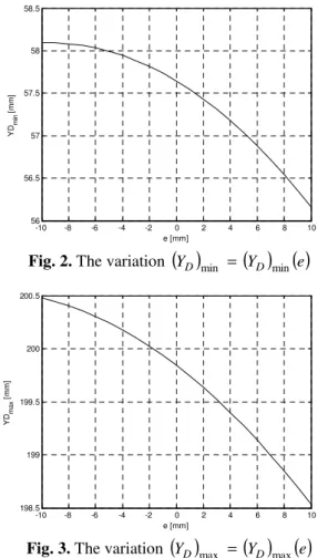
-10 -8 -6 -4 -2 0 2 4 6 8 10

56 56.5 57 57.5 58 58.5

e [mm]

Y

Dm

in

[

m

]

Fig. 2. The variation

( )

Y_D _min =

( ) ( )

Y_D _min e

-10 -8 -6 -4 -2 0 2 4 6 8 10

198.5 199 199.5 200 200.5

e [mm]

Y

Dm

a

x

[

m

]

( )

Y_D _max =

( ) ( )

Y_D _max e

Analyzing the Figures 2-4, one may observe that minimum and maximum values for the parameter YD decrease when the eccentricity e increases (negative values for e signify that the piston is in the left part of the Y-axis). The variation are small (up to one or two millimeters).

-10 -8 -6 -4 -2 0 2 4 6 8 10

9.2 9.4 9.6 9.8 10 10.2 10.4 10.6

e [mm]

ic

[

-]

Fig. 4. The variation i_c = i_c

( )

e

30 35 40 45 50 55

45 50 55 60 65 70 75

AB [mm]

Y

Dm

in

[

m

]

( )

Y_D _min =

( ) (

Y_D _min AB

)

30 35 40 45 50 55

180 185 190 195 200 205 210 215

AB [mm]

Y

Dm

a

x

[

m

]

( )

Y_D _max =

( ) (

Y_D _max AB

)

30 35 40 45 50 55

0 10 20 30 40 50 60

AB [mm]

ic

[

-]

(7)

118 120 122 124 126 128 130 132 134 136 138 57

58 59 60 61 62 63 64

BC [mm]

Y

Dm

in

[

m

]

( )

Y_D _min =

( ) (

Y_D _min BC

)

118 120 122 124 126 128 130 132 134 136 138 186

188 190 192 194 196 198 200 202 204

BC [mm]

Y

Dm

a

x

[

m

]

( )

Y_D _max =

( ) (

Y_D _max BC

)

118 120 122 124 126 128 130 132 134 136 138 5

6 7 8 9 10 11 12 13

BC [mm]

ic

[

-]

(

BC

)

The same variation is characteristic to the compression ratio (it decreases when the eccentricity increases), the variation being again a small one.

The influence of the length AB (Figs. 5-7)is more dramatically. The variation of the same parameters are situated in larger limits. The compression ratio may reach values of 50:1, which is impossible. In fact, we may conclude that the variation of AB assures a raw adjustment of the mechanism.

85 90 95 100 105 110

57 58 59 60 61 62 63

CA [mm]

Y

Dm

in

[

m

]

( )

Y_D _min =

( ) ( )

Y_D _min CA

85 90 95 100 105 110

188 190 192 194 196 198 200 202 204

CA [mm]

Y

Dm

a

x

[

m

]

( )

Y_D _max =

( ) ( )

Y_D _max CA

85 90 95 100 105 110

5 6 7 8 9 10 11 12 13

CA [mm]

ic

[

-]

( )

CA

20 22 24 26 28 30 32 34 36 38 40 45

50 55 60 65 70

OA [mm]

Y

Dm

in

[

m

]

(8)

20 22 24 26 28 30 32 34 36 38 40 185

190 195 200 205 210 215

OA [mm]

Y

Dm

a

x

[

m

]

( )

Y_D _max =

( ) ( )

Y_D _max OA

20 22 24 26 28 30 32 34 36 38 40 5

10 15 20 25 30 35 40

OA [mm]

ic

[

-]

( )

0A

90 95 100 105 110 115

56 56.5 57 57.5 58 58.5

CE [mm]

Y

Dm

in

[

m

]

( )

Y_D _min =

( ) ( )

Y_D _min CE

90 95 100 105 110 115

198 198.5 199 199.5 200 200.5

CE [mm]

Y

Dm

a

x

[

m

]

( )

Y_D _max =

( ) (

Y_D _max CE

)

90 95 100 105 110 115

8 8.5 9 9.5 10 10.5

CE [mm]

ic

[

-]

( )

CE

120 122 124 126 128 130 132 134 136 138 140 45

50 55 60 65 70

BD [mm]

Y

Dm

in

[

m

]

( )

Y_D _min =

( ) (

Y_D _min BD

)

120 122 124 126 128 130 132 134 136 138 140 185

190 195 200 205 210

BD [mm]

Y

Dm

a

x

[

m

]

( )

Y_D _max =

( ) (

Y_D _max BD

)

120 122 124 126 128 130 132 134 136 138 140 6

8 10 12 14 16 18 20 22 24 26

BD [mm]

ic

[

-]

(9)

76 78 80 82 84 86 88 90 92 94 96 57.59

57.6 57.61 57.62 57.63 57.64 57.65 57.66

d [mm]

Y

Dm

in

[

m

]

( )

Y_D _min =

( ) ( )

Y_D _min d

76 78 80 82 84 86 88 90 92 94 96 199.5

199.55 199.6 199.65 199.7 199.75 199.8 199.85 199.9 199.95 200

d [mm]

Y

Dm

a

x

[

m

]

( )

Y_D _max =

( ) ( )

Y_D _max d

76 78 80 82 84 86 88 90 92 94 96 9.7

9.75 9.8 9.85 9.9 9.95 10 10.05

d [mm]

ic

[

-]

Fig. 25. The variation i_c =i_c

( )

d

The rest of the figures may be similarly judged. One may observe that the length of the control lever CE has no influence on the extreme positions of the piston and the compression ratio, the length CE is set by constructive criteria.

Figure 26 presents the geometric locus of the point B when the control moves on vertical direction. In this situation, the variation of Y_E is

m 02 . 0

± . This zone influences the constructive dimensions of the engine.

Fig. 26. The geometric locus of the tiller's curve of the point B when YE is varied

7. CONCLUSION

The variations of the extreme positions of piston and of compression ratio are important in the synthesis of the mechanism.

The tiller curves for different characteristic points and dimensions of the elements give information about the constructive dimensions of the mechanism, relative positions of the elements etc.

REFERENCES

(10)

Viewpoint of Kinematic Structure, Journal of Mechanisms, Transmissions and Automation in Design, 1983.

[2] Hoeltgebaum, T., Simoni, R., Martins, D.,

Reconfigurability of engines: A kinematic approach to variable compression ratio engines, Mechanism and Machine Theory 96 (2016).

[3] Hara, V., Pandrea, N., Popa, D. Stan, M., Boncea, S., Motoare termice adaptative, Editura Universității din Pitești, 1995.

[4] Clenci, A., Autoturism echipat cu motor cu raport de comprimare variabil, Raport de cercetare, 2003.

[5] Miller, I., SAAB Variable Compression Motor, available online at www.me.udel.edu

/meeg425/SaabVarComp.doc, 2001.

[6] Mahlesh, P., J., Aparna, V., K., Variable compression ratio engine – A review of future power plant for automobile, International Journal of Mechanical Engineering Research and Development (IJMERD), Volume 2, Number 1 January- September 2012.

[7] Teodorczyk, A., Variable compression ratio engine VR/LE concept, published on

Institute of Heat Engineering Warsaw in 1995.

[8] Published at http://freerepublic.com/ focus/f-news/1818771/posts by Red Badger in 2007.

[9] SAE article http://articles.sae.org/6043/

published in 2009 by John Kendall.

[10] SAE article http://articles.sae.org/15040/

published in 2016by John Kendall.

[11] Nagarajaa, S., Sooryaprakashb, K., Sudhakaran, R., Investigate the Effect of Compression Ratio over the Performance and Emission Characteristics of Variable Compression Ratio Engine Fueled with Preheated Palm Oil -Diesel Blends, Procedia Earth and Planetary Science 11, 2015.

[12] Mănescu, B., Dragomir, I., Stănescu, N.-D., The Transitory Vibrations for a Variable Compression Ratio Mechanism, AVMS 2017, Timișoara, 2017.

[13] Teodorescu, P., P., Stănescu, N.-D., Pandrea, N., Numerical Analysis with Applications in Mechanics and Engineering, John Wiley & Sons, Hoboken, USA, 2013.

STUDIUL INFLUENŢEI PARAMETRILOR GEOMETRICI ASUPRA DEPLASĂRII PISTONULUI ŞI A RAPORTULUI DE COMPRIMARE PENTRU UN MECANISM CU COMPRIMARE VARIABILĂ Abstract: Se prezintă un mecanism cu raport de comprimare variabil şi se stabilesc relaţiile dintre diferiţi

parametri. Studiul este realizat în două moduri: prin abordare geometrică şi abordare multicorp. Pe baza formulelor deduse în cadrul acestui studiu, autorii determină poziţiile extreme ale pistonului, precum şi raportul de comprimare pentru anumiţi parametri geometrici. Variaţiile poziţiilor extreme şi ale raportului de comprimare în funcţie de variaţiile dimensiunilor elementelor sunt prezentate în mod grafic şi de aici se deduc concluziile. O atenţie deosebită este dată curbei de bielă pentru un punct specific al mecanismului.

Bogdan MĂNESCU, drd. ing., AKKA Romserv, București, Universitatea din Pitești,

Departamentul de Fabricație și Management Industrial, e-mail: [email protected], Office Phone: 0348453155,Home Phone 0766661647

Ionuț DRAGOMIR, drd. ing., AKKA Romserv, București, Universitatea din Pitești,

Departamentul de Fabricație și Management Industrial, e-mail: [email protected], Office Phone: 0348453155, Home Phone 0740950087

Nicolae-Doru Stănescu, prof. univ. dr. ing. habil. dr. mat., Universitatea din Pitești, Departamentul

de Fabricație și Management Industrial, e-mail: [email protected], [email protected], Office Phone: 0348453155, Home Address: Pitești, str. Matei Basarab, nr. 22, cod 110227, Home Phone 0745050055.

Nicolae PANDREA, prof. univ. emerit dr. ing., membru al Academiei de Științe Tehnice din