Available online throug
ISSN 2229 – 5046
DYSFUNCTION IN SMOOTH PURSUIT EYE MOVEMENT- A CASE STUDY OF
UNDAMPED FREE OSCILLATIONS
C. V. PAVANKUMAR*
(1)& N. Ch. PATTABHI RAMACHARYULU
(2)1
Faculty in Mathematics, Department of Humanities and Sciences,
Aurora’s Scientific and Technological Institute. Hyderabad. – 501301, India
2
Formerly Professor in Mathematics, National Institute of Technology, Warangal- 506004, India
(Received on: 13-01-13; Revised & Accepted on: 09-02-13)
ABSTRACT
T
his paper presents a simple deterministic model of dysfunctions of eye- tracking. The model is formulated as a second order nonlinear ordinary differential equation, incorporating non Hookesien cubic restoring force. The equation is solved analytically by employing a perturbation technique with the nonlinear restoring force coefficient as the perturbation parameter. Jump phenomena in angular displacement, angular velocity were discussed for wide spectrum of parameter values. Identified the equilibrium points of the model equation and stability of equilibrium points is also discussed.Key words: Pursuit Eye Tracking, Nonlinear Oscillations, Jump Phenomena.
1. INTRODUCTION
Dysfunctions [5, 10] in smooth pursuit eye movement are frequently encountered in schizophrenia patients [3], and also in some individuals with disorders of their central nervous system may be due to generic reasons [4]. The person suffering with such dysfunction would have to rotate the eye to track the signal which is coming from the periodically moving target [1],[2]. When the target motion is periodic the eye ball oscillations observed as a case study of undamped free oscillations [6]. This situation is modeled mathematically using a second order nonlinear ordinary differential equation of duffing type with a cubic non -Hooksian restoring force subject to non homogeneous initial conditions. An approximate solution of the modeled equation is obtained by employing a perturbation technique [9]. The perturbation parameter (ε) is characteristic of the nonlinearity of the restoring force. The angular displacement versus dimension less time profiles, the angular velocity versus dimensionless time profiles and phase plane portraits are illustrated for wide spectra of the perturbation parameter (ε), the initial angular displacement (a) and the initial angular velocity (b). A look at these illustrations shows the resonating character of both the angular displacement and angular velocity with the increase of initial data and increasing the coefficient of nonlinear restoring force, and spiral type of variations in the phase planes in the case of soft spring are discussed. The phenomenon of jump in dysfunction dynamic parameters angular displacement, angular velocity was discussed for wide spectrum of parameters and establishing the nonlinearity in the jump of dysfunction dynamic parameters using Lagrangian interpolation. Identified the equilibrium points of the model equation and stability of equilibrium points is also discussed.
Fig. 1: Schematic sketch of the eye ball movement under investigation
2. NOTATION ADOPTED
Φ : The angle between normal to the screen and the line connecting T he target’s position at time t, and the eye
I : Moment of inertia of the eye about the axis i.e. normal to the screen
STUDY OF UNDAMPED FREE OSCILLATIONS/IJMA- 4(2), Feb.-2013.
© 2013, IJMA. All Rights Reserved 143 α : The damping coefficient
k : Hooksian restoring constant
L : A nonlinear non hooksian restoring coefficient
A : peak to peak amplitude of the target moving periodically : The frequency of the target
3. MATHEMATICAL MODEL EQUATION
The deterministic eye dynamics in the presence of a target which is moving periodically, a nonlinear differential equation, is given by [perspectives in biological dynamics and theoretical medicine]
2
3
cos(
)
2
d
d
I
k
L
A
t
d
dt
dt
φ
+
α
φ
+
φ
−
φ
=
ω
(1)
(0)
, (0)
φ
=
α φ
•
=
β
(2) whereα
andβ
are the initial values of the angular displacement and initial angular velocity of the eye ball respectively.In terms of the following non dimensional parameters,
2
2
0
, ,
,
,
2 ,
,
0
0
2
2
0
0
0
0
0 0
L
k
d
A
t
I
I
I
I
ω
φ
φ
α
τ
ψ
ω
δ
ε
ω
φ
ω
ω
ω
ω φ
=
=
=
= Ω
=
=
= Γ
0 0
0
0 0
0
( ) ( ), (0) (0)
, t
a
τ
φ φ ψ φ φ ψ
ω α α φ ψ
φ
= =
= =
0 0 0 0
(0) (0), b
φ• =ω φ ψ• β ω φ=
(3)
By using (3) equation (1) can be reduced to
2
3 3
0 2 0 0 0
cos(
d)
d
d
I
k
L
A
t
dt
dt
ψ
ψ
ϕ
+
αϕ
+
ϕ ψ
−
ϕ ψ
=
ω
(4)2
2 3 3
0 0 2 0 0 0 0
0
cos( d )
d d
I k L A
d d
ψ ψ τ
ω ϕ αϕ ω ϕ ψ ϕ ψ ω
τ ω
τ + + − = (5)
2
3
2
cos(
)
2
d
d
d
d
ψ
δ
ψ
ψ εψ
τ
τ
τ
+
+ −
= Γ
Ω
(6)(7)
The coefficient ε signifies non Hooksian character of the nonlinear restoring force. This formulation signifies
undamped free oscillations of dysfunctions in eye movement take δ =0, ᴦ=0
The equation (4) reduces to
2
3
0
2
d
d
ψ ψ εψ
τ
+ −
=
(8)with initial conditions ψ(0)=a, (0)=bψ (9)
The spring is soft (or) hard accordingly ε is negative and positive respectively
4. ANALYTIC SOLUTION:
Let the
ψ τ ψ
( )
=
(0)
( )
τ εψ
+
(1)
( )
τ ε ψ
+
2
(2)
( ) . . .
τ
+
(10)Substituting (8) in the equation (6) and collecting the like powers of ε on both sides of equality we get the equations in the successive stages of approximation.
*
STUDY OF UNDAMPED FREE OSCILLATIONS/IJMA- 4(2), Feb.-2013.
5. THE BASIC (OR) ZERO TH ORDER APPROXIMATION
In this approximation the equation to be solved is
(0)
2
(0)
0
2
d
d
ψ
ψ
τ
+
=
(11)
With the initial conditions
ψ
(0)
(0)
=
a
,
ψ
(0)
•
(0)
=
b
(12)This yields the solution isψ(0)( )τ =acos( )τ +bsin( )τ (13)
6. THE FIRST ORDER APPROXIMATION
The equation for
ψ
(1)
( )
τ
is2 (1)
(1)
3
( cos
sin )
2
d
a
b
d
ψ
ψ
τ
τ
τ
+
=
+
(14)With initial conditions
ψ
(1)
(0)
=
0, (0)
ψ
•
(1)
=
0
(15)The solution of equation (14) satisfying the initial conditions in (15) is
3
2
3
2
3
2
(
3
)
9(
5
)
(
3
)
(1)
( )
cos
sin
cos3
32
32
32
2
3
3
2
3
2
(3a
)
(3
3
)
(3
3
)
-
sin 3
cos
sin
32
8
8
a
a b
b
a b
a
a b
b b
b
a b
a
ab
ψ
τ
τ
τ
τ
τ
τ
τ
τ
τ
−
+
−
=
+
−
−
−
+
+
+
(16)
Hence up to this order of approximation the angular displacement is given by
(0)
(1)
( )
( )
t
( )
ψ τ ψ
=
+
εψ
τ
(17)
3
2
3
2
3
2
(
3
) cos
9(
5
)sin
(
3
) cos 3
( ) ( cos
sin )
2
3
3
2
3
2
32 -(3a
)sin 3
4(3
3
) cos
4(3
3
) sin
a
a b
b
a b
a
a b
a
b
b b
b
a b
a
ab
τ
τ
τ
ε
ψ τ
τ
τ
τ
τ
τ
τ τ
−
+
+
−
−
=
+
+
−
−
+
+
+
(18)And the angular velocity is given by
3 2 3 2 3 2
( 3 ) sin 9( 5 ) s 3( 3 ) sin 3
2 3 3 2
( ) ( sin s ) -3(3a ) s 3 4(3 3 )(cos sin ) 32
3 2
4(3 3 ) (cos sin )
a a b b a b co a a b
a bco b b co b a b
a ab
τ τ τ
ε
ψ τ τ τ τ τ τ τ
τ τ τ
− − + + + −
• = − + + − − + −
+ + +
(19)
7. THE ANGULAR DISPLACEMENT VERSES TIME PROFILES FOR DIFFERENT VALUES OF PARAMETERS ARE GIVEN BELOW
0 10 20 30 40 50 60 70 80 90 100
-1.5 -1 -0.5 0 0.5 1 1.5x 10
-3
-- dimension
less-time- --angl ar di s pl ac em ent -ε=0.001,a=0.001,b=0.001
STUDY OF UNDAMPED FREE OSCILLATIONS/IJMA- 4(2), Feb.-2013.
© 2013, IJMA. All Rights Reserved 145
0 10 20 30 40 50 60 70 80 90 100
-1.5 -1 -0.5 0 0.5 1 1.5
---dimensionless
time-
---angul
ar
di
s
pl
ac
em
ent
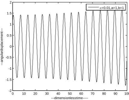
-ε=0.001,a=1,b=1
Fig. 3: variation of angular displacement versus time for the nonlinear restoring coefficient ε=0.001, initial angular displacement a=1 and initial angular velocity b=1. For this parameter values the amplitude of angular displacement is not changing as time increases.
0 10 20 30 40 50 60 70 80 90 100
-150 -100 -50 0 50 100 150
---dimensionless
time-
---angul
ar
di
s
pl
ac
em
ent
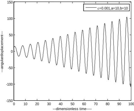
-ε=0.001,a=10,b=10
Fig. 4: variation of angular displacement versus time for the nonlinear restoring coefficient ε=0.001, initial angular displacement a=10 and initial angular velocity b=10. For this parameter values the amplitude of angular displacement is increasing as time increases.
0 10 20 30 40 50 60 70 80 90 100
-1.5 -1 -0.5 0 0.5 1 1.5x 10
-3
---dimensionless
time-
---angul
ar
di
s
pl
ac
em
ent
-ε=0.01,a=0.001,b=0.001
STUDY OF UNDAMPED FREE OSCILLATIONS/IJMA- 4(2), Feb.-2013.
0 10 20 30 40 50 60 70 80 90 100
-2 -1.5 -1 -0.5 0 0.5 1 1.5 2
-dimensionlesstime-
---angul
ar
di
s
pl
ac
em
ent
-ε=0.01,a=1,b=1
Fig. 6: variation of angular displacement versus time for the nonlinear restoring coefficient ε=0.01, initial angular displacement a=1 and initial angular velocity b=1. For this parameter values the amplitude of angular displacement is increasing as time increases.
0 10 20 30 40 50 60 70 80 90 100
-1500 -1000 -500 0 500 1000 1500
-dimensionlesstime-
---angul
ar
di
s
pl
ac
em
ent
--ε=0.01,a=10,b=10
Fig. 7: variation of angular displacement versus time for the nonlinear restoring coefficient ε=0.01, initial angular displacement a=10 and initial angular velocity b=10. For this parameter values the amplitude of angular displacement is increasing rapidly as time increases.
8. PHASE PLANE PORTRAITS
The angular velocity versus angular displacement profiles (analytical phase plane portraits) are given for different values of parameter
-1.5 -1 -0.5 0 0.5 1 1.5
x 10-3 -1.5
-1 -0.5 0 0.5 1 1.5x 10
-3
-angulardisplacement
--angul
ar
-v
el
oc
it
y
-ε=0.01,a=0.001,b=0.001
STUDY OF UNDAMPED FREE OSCILLATIONS/IJMA- 4(2), Feb.-2013.
© 2013, IJMA. All Rights Reserved 147
-2 -1.5 -1 -0.5 0 0.5 1 1.5 2
-2 -1.5 -1 -0.5 0 0.5 1 1.5 2 ---angular displacement ---angul ar v el oc it y -ε=0.01,a=1,b=1
Fig. 9:variation of angular velocity versus angular displacement for the nonlinear restoring coefficient ε=0.01, initial
angular displacement a=1and initial angular velocity b=1
-1500 -1000 -500 0 500 1000 1500
-1500 -1000 -500 0 500 1000 1500 ---angular displacement ---angul ar v el oc it y -ε=0.01,a=10,b=10
Fig. 10:variation of angular velocity versus angular displacement for the nonlinear restoring coefficient ε=0.01, initial
angular displacement a=10and initial angular velocity b=10.
9. JUMP PHENOMINA IN PEAK TO PEAK AMPLITUDE OF DYSFUNCTION DYNAMIC PARAMETERS -ANGULAR DISPLACEMENT AND ANGULAR VELOCITY
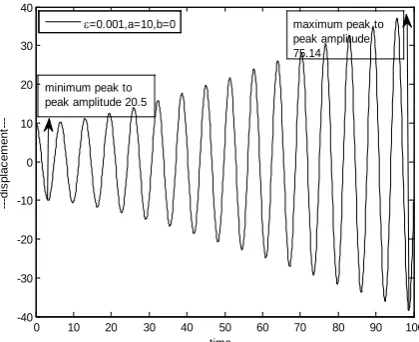
The dysfunction dynamical parameters angular displacement and angular velocity are simulated in the time interval [0,100] using the analytical solution of the model (18), (19) and using the software MATLAB. For different values of the parameters in the model such as initial angular displacement, initial angular velocity and coefficient of nonlinear restoring force are taken at different levels and using the analytical solution of the model. Jump in peak to peak amplitude of The dysfunction dynamical parameters angular displacement and angular velocity calculated as shown in the Fig (11).
0 10 20 30 40 50 60 70 80 90 100
-40 -30 -20 -10 0 10 20 30 40 time ---di s pl ac em ent -ε=0.001,a=10,b=0
minimum peak to peak amplitude 20.5
maximum peak to peak amplitude 75.14
STUDY OF UNDAMPED FREE OSCILLATIONS/IJMA- 4(2), Feb.-2013.
10. JUMP PHENOMINA IN PEAK TO PEAK AMPLITUDE OF DYSFUNCTION DYNAMIC PARAMETERS -ANGULAR DISPLACEMENT:
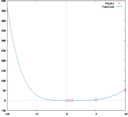
The Nonlinear restoring coefficient ε is taken in three levels(0.001,0.01,0.1,1) together with no initial angular displacement and varying the initial angular velocity( b),Then The jump in peak to peak amplitude in angular displacement is function of initial angular velocity (b). The graph of Lagrangian interpolated polynomial is given for each case, by taking the values of parameter (b) taken on x-axis and the corresponding jump in peak to peak amplitude taken on Y-axis.
Table: 1
ε a b Minimum value of peak to peak amplitude
Maximum value of peak to peak amplitude
Jump in peak to peak amplitude
0.001 0 0.1 0.2 0.2 0
0.001 0 0.5 1 1 0
0.001 0 1 2 2 0
0.001 0 5 10.064 13.8 3.736
0.001 0 10 20.5 75.14 54.64
0.001 0 15 32 235 203
0.001 0 25 63 1106 1043
0.001 0 50 310 8818 8508
Table: 1 Table gives the values of minimum and maximum values of peak to peak amplitude and corresponding jump
in peak to peak amplitude in angular displacement when ε=0.001, initial angular displacement (a=0) and with varying
angular velocity
Fig. 12: When nonlinear restoring coefficient ε =0.001, with no initial angular displacement and initial angular displacement (b) is changing . The jump is linear up to b=5 and then it is nonlinear.
Table: 2
ε a b Minimum value of peak to peak amplitude
Maximum value of peak to peak amplitude
Jump in peak to peak amplitude
0.01 0 0.1 0.2 0.2 0
0.01 0 0.5 1 1 0
0.01 0 1 2 2 0
0.01 0 5 10.746 90 79.254
0.01 0 10 32 720 688
0.01 0 15 84 2500 2416
0.01 0 25 366 11826 11460
0.01 0 50 2824 88240 85416
Table 2: Table gives the values of minimum and maximum values of peak to peak amplitude and corresponding jump
in peak to peak amplitude in angular displacement when ε=0.01 , initial angular displacement (a=0) and with varying
STUDY OF UNDAMPED FREE OSCILLATIONS/IJMA- 4(2), Feb.-2013.
© 2013, IJMA. All Rights Reserved 149 Fig. 13: When nonlinear restoring coefficient ε =0.01, with no initial angular displacement initial angular displacement (b) is changing. The jump is linear up to b < 5 and then it is nonlinear.
Table: 3
ε a b Minimum value of peak to peak amplitude
Maximum value of peak to peak amplitude
Jump in peak to peak amplitude
0.1 0 0.1 0.2 0.2 0
0.1 0 0.5 1 1.3744 0.3744
0.1 0 1 2.05 7.514 5.464
0.1 0 5 31 921.8 890.8
0.1 0 10 234 7058 6824
0.1 0 15 761.2 24200 23438.8
0.1 0 25 3546 114300 110754
0.1 0 50 29060 942400 913340
Table: 3 Table gives the values of minimum and maximum values of peak to peak amplitude and corresponding jump in peak to peak amplitude in angular displacement when ε=0.1, initial angular displacement (a=0) and with varying angular velocity.
Fig. 14:When nonlinear restoring coefficient ε =0.1, with no initial angular displacement initial angular displacement (b) is changing. The jump is linear up to when b < 2 and then it is nonlinear.
Table: 4
ε a b Minimum value of peak to peak amplitude
Maximum value of peak to peak amplitude
Jump in peak to peak amplitude
1 0 0.1 0.2004 0.2138 0.0134
1 0 0.5 1.0746 9.486 8.4114
1 0 1 3.094 76.74 73.646
1 0 5 294.6 9224 8929.4
1 0 10 2336 74580 72244
1 0 15 3924 242200 238276
1 0 25 36780 1183000 1146220
STUDY OF UNDAMPED FREE OSCILLATIONS/IJMA- 4(2), Feb.-2013.
Table: 4 Table gives the values of minimum and maximum values of peak to peak amplitude and corresponding jump in peak to peak amplitude in angular displacement when ε=1, initial angular displacement (a=0) and with varying angular velocity.
Fig. 15:When nonlinear restoring coefficient ε =1, with no initial angular displacement initial angular displacement (b) is changing. The jump is linear up to b < 1 and then it is nonlinear.
11. JUMP PHENOMENA WHEN NO TAKE OFF ANGULAR VELOCITY
The Nonlinear restoring coefficient ε is taken in three levels(0.001,0.01,0.1,1) together with no initial angular velocity(b), and changing the initial angular displacement(a) then jump in peak to peak amplitude in angular displacement is function of initial angular displacement (a). The graph of Lagrangian interpolated polynomial is given for each case, by taking The values of parameter (a) taken on x-axis and the corresponding jump in peak to peak amplitude taken on Y-axis.
Table: 5
ε a b Minimum value of peak to peak amplitude
Maximum value of peak to peak amplitude
Jump in peak to peak amplitude
0.001 0.1 0 0.2 0.2 0
0.001 0.5 0 1 1 0
0.001 1 0 2 2 0
0.001 5 0 10 13.7 3.7
0.001 10 0 20 76.74 56.74
0.001 15 0 31.08 251.8 220.72
0.001 25 0 49.62 1160.2 1110.58
0.001 50 0 146.1 9268 9121.9
Table: 5 Table gives the values of minimum and maximum values of peak to peak amplitude and corresponding jump
in peak to peak amplitude in angular displacement when ε=0.001, initial angular velocity (b=0) and with varying angular displacement.
STUDY OF UNDAMPED FREE OSCILLATIONS/IJMA- 4(2), Feb.-2013.
© 2013, IJMA. All Rights Reserved 151 Table: 6
ε a b Minimum value of peak to peak amplitude
Maximum value of peak to peak amplitude
Jump in peak to peak amplitude
0.01 0.1 0 0.2 0.2 0
0.01 0.5 0 1 1 0
0.01 1 0 2 2.216 0.126
0.01 5 0 11.952 93.18 81.228
0.01 10 0 60.46 741.8 680.74
0.01 15 0 114.74 2502 2387.26
0.01 25 0 547.8 11588 11040.2
0.01 50 0 1531.4 92720 91188.6
Table: 6 Table gives the values of minimum and maximum values of peak to peak amplitude and corresponding jump in peak to peak amplitude in angular displacement when ε=0.01, initial angular velocity (b=0) and with varying angular displacement.
Fig. 17: When nonlinear restoring coefficient ε =0.01, with no initial angular velocity and with varying angular displacement (a). The jump is linear up to b<5 and then it is nonlinear.
Table: 7
ε a b Minimum value of peak to peak amplitude
Maximum value of peak to peak amplitude
Jump in peak to peak amplitude
0.1 0.1 0 0.2 0.2 0
0.1 0.5 0 1 1.3574 0.3574
0.1 1 0 2 7.674 5.674
0.1 5 0 42.7 926.8 884.1
0.1 10 0 354.6 7418 7063.4
0.1 15 0 1169.8 25040 23870.2
0.1 25 0 5218 115900 110682
0.1 50 0 44540 927200 882660
STUDY OF UNDAMPED FREE OSCILLATIONS/IJMA- 4(2), Feb.-2013.
Fig. 18: When nonlinear restoring coefficient ε =0.1, with no initial angular velocity and with varying angular displacement (a). The jump is linear up to b<1 and then it is nonlinear.
Table: 8
ε a b Minimum value of peak to peak amplitude
Maximum value of peak to peak amplitude
Jump in peak to peak amplitude
1 0.1 0 0.2 0.2 0
1 0.5 0 1.1984 9.318 8.1196
1 1 0 3.84 74.1 70.26
1 5 0 444.6 9272 8827.4
1 10 0 3562 74180 70618
1 15 0 12028 250400 238372
1 25 0 55700 1159000 1103300
1 50 0 445600 9272000 8826400
Table: 8 Table gives the values of minimum and maximum values of peak to peak amplitude and corresponding jump in peak to peak amplitude in angular displacement when ε=1, initial angular velocity (b=0) and with varying angular displacement.
STUDY OF UNDAMPED FREE OSCILLATIONS/IJMA- 4(2), Feb.-2013.
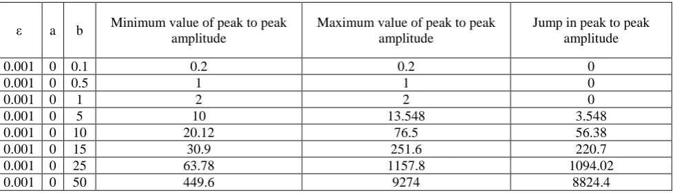
© 2013, IJMA. All Rights Reserved 153 12. .JUMP PHENOMINA IN PEAK TO PEAK AMPLITUDE OF DYSFUNCTION DYNAMIC PARAMETER - ANGULAR VELOCITY
Table: 9
ε a b Minimum value of peak to peak amplitude
Maximum value of peak to peak amplitude
Jump in peak to peak amplitude
0.001 0 0.1 0.2 0.2 0
0.001 0 0.5 1 1 0
0.001 0 1 2 2 0
0.001 0 5 10 13.548 3.548
0.001 0 10 20.12 76.5 56.38
0.001 0 15 30.9 251.6 220.7
0.001 0 25 63.78 1157.8 1094.02
0.001 0 50 449.6 9274 8824.4
Table: 9 Table gives the values of minimum and maximum values of peak to peak amplitude is and corresponding jump in peak to peak amplitude in angular velocity when ε=0.001, initial angular displacement (a=0) and with varying angular displacement(a).
Fig. 20When nonlinear restoring coefficient ε =0.001, with no initial angular displacement and with varying angular
velocity (b). The jump is linear up to b=5 and then it is nonlinear.
Table: 10
ε a b Minimum value of peak to peak amplitude
Maximum value of peak to peak amplitude
Jump in peak to peak amplitude
0.01 0 0.1 0.2 0.2 0
0.01 0 0.5 1 1 0
0.01 0 1 1.998 2.128 0.13
0.01 0 5 10.408 93.1 82.692
0.01 0 10 35.7 741.4 705.7
0.01 0 15 120.6 2504 2383.4
0.01 0 25 578.2 11596 11017.8
0.01 0 50 4664 92780 88116
STUDY OF UNDAMPED FREE OSCILLATIONS/IJMA- 4(2), Feb.-2013.
Fig. 21 When nonlinear restoring coefficient ε =0.01, with no initial angular displacement and with varying angular
velocity (b). The jump is linear up to b<5 and then it is nonlinear.
Table: 11
ε a b Minimum value of peak to peak amplitude
Maximum value of peak to peak amplitude
Jump in peak to peak amplitude
0.1 0 0.1 0.2 0.2 0
0.1 0 0.5 1 1.3528 0.3528
0.1 0 1 2.012 7.65 5.638
0.1 0 5 44.96 927.4 882.44
0.1 0 10 370.8 7422 7051.2
0.1 0 15 1265.8 25040 23774.2
0.1 0 25 5910 115960 110050
0.1 0 50 47260 927800 880540
Table: 11 Table gives the values of minimum and maximum values of peak to peak amplitude is and corresponding jump in peak to peak amplitude in angular velocity when ε=0.1, initial angular displacement (a=0) and with varying angular velocity(b).
Fig. 22 When nonlinear restoring coefficient ε =0.1, with no initial angular displacement and with varying angular
velocity (b). The jump is linear up to b=1 and then it is nonlinear.
Table: 13
ε a b Minimum value of peak to peak amplitude
Maximum value of peak to peak amplitude
Jump in peak to peak amplitude
1 0 0.1 0.19972 0.2126 0.01288
1 0 0.5 1.0296 9.31 8.2804
1 0 1 3.57 74.14 70.57
1 0 5 469.2 9278 8808.8
1 0 10 3786 74220 70434
1 0 15 12788 250400 237612
1 0 25 59100 1159600 1100500
STUDY OF UNDAMPED FREE OSCILLATIONS/IJMA- 4(2), Feb.-2013.
© 2013, IJMA. All Rights Reserved 155 Table: 12 Table gives the values of minimum and maximum values of peak to peak amplitude and corresponding
jump in peak to peak amplitude in angular velocity when ε=1, initial angular displacement (a=0) and with varying
angular velocity(b).
Fig. 23 When nonlinear restoring coefficient ε =1, with no initial angular displacement and with varying angular velocity (b). The jump is linear up to b=0.5 and then it is nonlinear.
Table: 13
ε a b Minimum value of peak to peak amplitude
Maximum value of peak to peak amplitude
Jump in peak to peak amplitude
0.001 0.1 0 0.2 0.2 0
0.001 0.5 0 1 1 0
0.001 1 0 2 2 0
0.001 5 0 9.938 13.4 3.462
0.001 10 0 20 75.14 55.14
0.001 15 0 30.76 247.6 216.84
0.001 25 0 76.14 1141 1064.86
0.001 50 0 602.4 9132 8529.6
Table: 13 Table gives the values of minimum and maximum values of peak to peak amplitude and corresponding
jump in peak to peak amplitude in angular velocity when ε=0.001, initial angular velocity (b=0) and with varying angular displacement(a).
STUDY OF UNDAMPED FREE OSCILLATIONS/IJMA- 4(2), Feb.-2013.
Table: 14
ε a b Minimum value of peak to peak amplitude
Maximum value of peak to peak amplitude
Jump in peak to peak amplitude
0.01 0.1 0 0.2 0.2 0
0.01 0.5 0 0.9992 1.0034 0.0042
0.01 1 0 2 2.128 0.128
0.01 5 0 10.384 91.6 81.216
0.01 10 0 46.96 730.4 683.44
0.01 15 0 162.28 2466 2303.72
0.01 25 0 420.4 11414 10993.6
0.01 50 0 3578 91320 87742
Table: 14 Table gives the values of minimum and maximum values of peak to peak amplitude and corresponding
jump in peak to peak amplitude in angular velocity when ε=0.01, initial angular velocity (b=0) and with varying angular displacement(a).
Fig. 25 When nonlinear restoring coefficient ε =0.01, with no initial angular velocity (b) and with varying angular displacement (a). The jump is linear up b=0.5and then it is nonlinear.
Table: 15
ε a b Minimum value of peak to peak amplitude
Maximum value of peak to peak amplitude
Jump in peak to peak amplitude
0.1 0.1 0 0.2 0.2 0
0.1 0.5 0 0.9938 1.34 0.3462
0.1 1 0 2 7.514 5.514
0.1 5 0 32.30 913.2 880.9
0.1 10 0 279.8 7306 7026.2
0.1 15 0 956.2 24660 23703.8
0.1 25 0 4512 114160 109648
0.1 50 0 36320 913200 876880
Table: 15 Table gives the values of minimum and maximum values of peak to peak amplitude and corresponding
STUDY OF UNDAMPED FREE OSCILLATIONS/IJMA- 4(2), Feb.-2013.
© 2013, IJMA. All Rights Reserved 157 Fig. 26 When nonlinear restoring coefficient ε =0.1, with no initial angular velocity (b) and with varying angular displacement (a). The jump is linear up to b=0.1 and then it is nonlinear.
Table: 16
ε a b Minimum value of peak to peak amplitude
Maximum value of peak to peak amplitude
Jump in peak to peak amplitude
1 0.1 0 0.2 0.2 0
1 0.5 0 0.9486 9.16 8.2114
1 1 0 4.696 73.04 68.344
1 5 0 359.2 9132 8772.8
1 10 0 2900 73060 70160
1 15 0 9786 246600 236814
1 25 0 45360 1141600 1096240
1 50 0 363000 9132000 8769000
Table: 16 Table gives the values of minimum and maximum values of peak to peak amplitude and corresponding
jump in peak to peak amplitude in angular velocity when ε=1, initial angular velocity (b=0) and with varying angular displacement(a).
STUDY OF UNDAMPED FREE OSCILLATIONS/IJMA- 4(2), Feb.-2013.
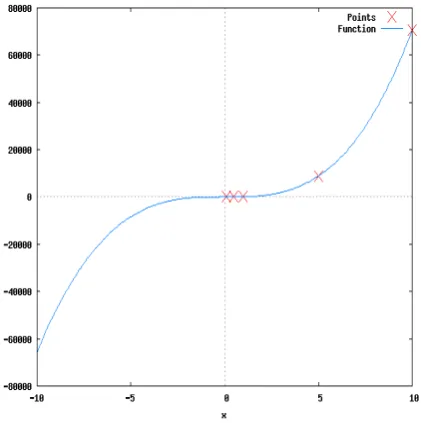
13. STABILITY ANALYSIS The differential equation
2
3
0
2
d
d
ψ ψ εψ
τ
+ −
=
(20)The above differential equation divided into two first order differential equations d
y d
ψ
τ = (21)
3
dy
dτ =
εψ
−ψ
(22) The system has the following four equilibrium states (i)-(iii) resulting fromd y d
ψ
τ = = 0;
3
dy
dτ =
εψ
−ψ
= 0 (23) E1: state in which both angular displacement angular velocity are zeroψ
= 0;y
= 0 (24)E2: The state in which only the angular displacement is not equal to zero
And angular velocity is equal to zero
ψ
= ± (1/√ε);y
= 0(25)
14. STABILITY OF THE EQUILIBRIUM STATES
15. Stability of the Equilibrium State E1:
ψ
= 0;y
= 0.We consider slight deviations u1 (τ) and u2 (τ) over the steady state (
ψ
,y
)ψ
=ψ
+ u1 (τ) (26)y
=y
+ u2 (τ) (27) Where u1 (τ) and u2 (τ) are small so that terms other than the first order can be neglected.By substituting (2.26) and (2.27) in (2.21) and (2.22) we get
1
2
du
y
u
d
τ
= +
(28)2 3
3
3
2
2
[( )
3( )
( )
] ( )
1
1
1
1
du
u
u
u
u
d
τ
=
ε ψ
+
ψ
+ψ
+−
ψ
−
(29) By neglecting products and second and higher powers of u1 and u2, we get
1
du
d
τ
= u2; 2du
d
τ
= -u1 (30) ;(31)Whose roots are ±i , both the roots are complex. Hence the steady state is unstable. Further from (30) and (31) we get
cos
sin
1
10
20
STUDY OF UNDAMPED FREE OSCILLATIONS/IJMA- 4(2), Feb.-2013.
© 2013, IJMA. All Rights Reserved 159
sin
cos
2
10
20
u
= −
u
τ
+
u
τ
(33)Where u10, u20 are initial values of u1, u2 respectively and the solution curves are shown in Figures 28 to 31 and the conclusions are presented below.
16. Stability of the equilibrium states E2,E3:
ψ
=1
ε
±
;y
= 0By substituting (2.26) and (2.27) in (2.21) and (2.22) we get
1
2
du
y
u
d
τ
= +
(34)2 3
3
3
2
2
[( )
3( )
( )
] ( )
1
1
1
1
du
u
u
u
u
d
τ
=
ε ψ
+
ψ
+ψ
+−
ψ
−
(35)By neglecting products and second and higher powers of u1 and u2, the corresponding linearised perturbed equations are
1 2
du
u
d
τ
=
(36)2 1
2
du
u
d
τ
=
(37)Whose roots are ±√2 both the roots are real and opposite. Hence the steady state is unstable .The solutions of equations (36) and (37) are given by
20 20 20 20
10 10 10 10
2 2 2 2
1 2
2 2 2 2
( ) ( )
2 2 2 2
u u u u
u u u u
u τ e τ e− τ and u τ e τ e− τ
+ − + −
= + = −
(38)
0 10 20 30 40 50 60 70 80 90 100
-1.5 -1 -0.5 0 0.5 1 1.5
---dimension less
time-
--- u1 and --
u2-
--u1 u2
STUDY OF UNDAMPED FREE OSCILLATIONS/IJMA- 4(2), Feb.-2013.
-1.5 -1 -0.5 0 0.5 1 1.5
-1.5 -1 -0.5 0 0.5 1 1.5
---u1--- u
2
---Fig. 29: Trajectories of perturbed angular displacement u1(τ) and angular velocity u2(τ) at E1
0 0.2 0.4 0.6 0.8 1 1.2 1.4 1.6 1.8 2
0 5 10 15 20 25
---dimension less
time-
--- u1 and --
u2-
--u1 u2
Fig. 30: variation of u1 (τ) and u2 (τ) versus dimensionless time at equilibrium E3and E4
0 1 2 3 4 5 6
x 105 0
1 2 3 4 5 6 7 8x 10
5
----u1--- u
2
---Fig. 31: Trajectories of perturbed angular displacement u1 (τ) and angular velocity u2(τ) at E2 and E3
CONCLUSIONS
(1) The resonating character in both the dysfunction dynamic parameters (angular displacement, angular velocity) is increasing with increasing of initial data and the coefficient of nonlinear restoring force(ε).
(2) The Lagrangian interpolating patterns showing that the jump in peak to peak amplitude is Linear for lower values of initial data and lower values of non linear restoring coefficient, the nonlinearity appears in early stages with increase of
parameters (a,b,ε).
REFERENCES
[1] N. Ch. Pattabhi Ramacharyulu, C.V. Pavankuma Nonlinear damped oscillations and a case study of dysfunctions in eye tracking -I. arpn journal of engineering and applied sciences.
STUDY OF UNDAMPED FREE OSCILLATIONS/IJMA- 4(2), Feb.-2013.
© 2013, IJMA. All Rights Reserved 161 [3] Couch FH, Fox JC Photographic study of ocular movements in mental disease. Arch Neural Psychiatry. (1934), volume: 34, PP: 556-578.
[4] Defender AR, Dodge R ‘An experimental study of the ocular reactions of the insane from hotographic records’, Brain, (1908) ,volume:31, PP: 451-489.
[5] Holzman P.S, Proctor L.R, Hughes D.W ‘Eye tracking patterns in Schizophrenia’ (1973) Science, volume: 181, PP: 179-181.
[6] Huberman. B. A, Crutchfield J. P ‘Chaotic States of An harmonic Systems in Periodic Fields’(1979), phy. lett, volume:.43, PP:1743-1747.
[7] Nafeh and Mook ‘Non linear oscillations’, John Wiley and sons, (1995).
[8] Tomer R, Mintz M, Levy A, Myslobodsky M.‘ Smooth pursuit pattern in schizophrenic patients during cognitive task’, ( 1981), Bio Psychiatry , volume:2, PP:131-44.
[9] Chaotic Vibrations: an Introduction for Applied Scientists and Engineers Francis C. Moon, John Wiley & Sons.
Source of support: Nil, Conflict of interest: None Declared