Available online at:
www.ijamee.info
RESEARCH ARTICLE
Jeffrey E Jarrett & Yifei Li | May 2016 | Vol.3| Issue 5|01-13
Characteristics of the Association Some Asian Equity Markets
with the New York and London Equity Market
Jeffrey E Jarrett*, Yifei Li
Management Science and Finance, University of Rhode Island, Kingston, RI (USA)
Abstract
We compare Equity Markets (Hong Kong and one market in China, PRC) with the New York and London Equity Markets (two mature Western markets), with respect to volatility and rates of return. The purpose is to improve and increase our knowledge of the covariation of these markets. Utilization of exploratory data analysis, cross-correlation analysis and identification of the auto-regressive integrated moving-average (ARIMA) models for analysis and possible model predication. No previous research is as current and definitive as accomplished in this study on data collected over long periods of time from the sources utilized. The analysis indicates that use of data analytical methods provides evidence as to the cointegration of financial markets.
Keywords: Exploratory Data Analysis, Cross Correlation Analysis, ARIMA modeling.
Introduction
Previous studies of comparisons of Asian equity markets Western equity markets include Chow, et al. [1], Chen [2], Cheung and Ng [3], Liaw [3], and Jarrett and Sun [4]. These studies focused on describing China (PRC) as a new opportunity as a new opportunity for Western investment and growing returns to outside investors.
They utilized criteria for analyzing for analyzing Western equity markets [5-8]. Furthermore, Chow and Lawler [9]; (Data up to 2002) and later Jarrett and Sun using a newer data set 2012, analyzed the price indexes for the Shanghai equity market in comparison with the New York (NYSE) equity market. The last study divided the very lengthy time period into three sub periods to achieve a temporal analysis as well. Other studies including Baily et al. 2009, Jarrett and Sun 2009A and 2009B focused on other issues in Chinese equity markets due to huge and development of the Shenzhen and Shanghai equity markets of China (PRC). Last, Jarrett, Klein and Kyper [10] studied New York, London, and the two large China (PRC) equity markets doing both a study of temporal activity and how they effectively correlate with each other.
Another question relates to the equity market of Hong Kong (a.k.a., Hang Seng market). Previously, Pan, Li and Jarrett [11] studied the relationship of high frequency interactions between China A-shares and Hong Kong H-A-shares of dual-listed firms. This special study indicated the correlation of these two types of shares. Since Hong Kong and China have strong economic and market relationships, we wish to determine how these special relationships
In the next section, we intend to show exploratory graphical data to explain the variation in characteristics in characteristics of the distribution of price index data and the distribution of volume for the same equity markets. In turn, we explain by auto-regressive modeling the relation between volume and lagged variables of order 1 and 2 for three exchanges. Not enough data was available for the fourth equity market (Shanghai).
Jeffrey E Jarrett & Yifei Li | May 2016 | Vol.3| Issue 5|01-13 lagged variables. In the next analysis, we
investigate the cross-correlation of the three equity markets (New Yoke, London and Hong Kong) and last, we determine the ARIMA model for each variable studied. The conclusions will indicate covariation, temporal analysis and results for both closing prices and volume.
The Analysis of Volume
To begin, we observe the cross-correlation among the volume of shares denoted by
HKvol (Hong Kong), LTvol (London) and
NYvol (New York) in Table 1. These data begin with descriptive statistics of the size of data sets, mean and standard of values along with their minimum and maximum values. Most important, the measure of variation (standard deviation) of volume and its span (maximum minus minimum
surpasses the same statistics for LT vol and NYvol. There is (indirect) negative association between LTvol and NYvol (-0.48434). Finally, HKvol and NYvol have positive (direct) association of 0.92481. Such a large coefficient indicates great strength in this relationship. Next, we investigate to find further evidence of this phenomenon.
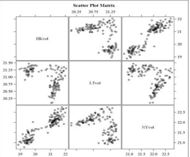
Observe Figure 1, the Scatter Plot Matrix
of the Volume Cross-Correlation among exchanges. The bottom left plot for association between HKvol and NYvol
appears to have best plot of positive linear relationship, that is, as volume increases in one exchange, the send exchange increase at a pace similar to the first. The top right hand graph shows the same outcome because it shows the plot of the same data.
Figure 1: Scatter plot matrix volume cross-correlations among exchanges
For the price data, we observe data on four exchanges by including Shanghai (The largest equity market in China, PRC.) to add additional evidence to the observed relationship evidence to the observed relationships among them. The mean closing pricing price for Hong Kong (HK15pre) is
Shanghai having the largest spread, Hong Kong the smallest spread ND London and New York in the middle. Finally, observing the correlations among the closing price for each equity market yield for each equity market yield a different picture than for volume. The correlation coefficients for all
two-by-two comparisons ranged from 0.78945 for LTprc – SHprc to 0.94814 for
NYprc – SHprc. These large values for the one-by-one comparison indicate the strong association of closing prices among the equity markets to another with London and Shanghai markets most correlated with each other.
Table 1: Regression results for Hong Kong, London and New York stock exchange
Hong Kong (Hang Seng) Exchange
Parameter Estimates
Variable Parameter Standard Error t-statistic P-value
Estimate
Intercept 1 -77281 5423.799 -14.25 .0001
vol 1 2111.140 1070.762 1.97 .0505
vol1 1 1286.042 1295.059 0.99 .3223
Vol2 1 1214.615 1058.466 1.15 .2530
Root MSE 2932.634 R-square 0.6779
Dependent Mean 1
7 682
Adj R-square 0.6713
Coeff Var 16.585
London Exchange
Parameter Estimates
Variable Parameter Standard Error t-statistic P-value
Estimate
Intercept 1 26396 4022.606 --3.49 .0001
vol 1 -441.416 396.817 -1.11 .0206
vol1 1 -372.327 442.483 -0.84 .4017
Vol2 1 -186.722 394.545 -0.47 .6368
Root MSE 739.597 R-square 0.1498
Dependent
Mean 5430.490 Adj R-square 0.1566
Coefficient of Variation 13.619
New York Stock Exchange (NYSE)
Parameter Estimates
Variable of Parameter Standard Error t-statistic P-value Estimate
Intercept 1 -15822 4532.583 -3.49 .0006
vol 1 951.492 749.618 1.27 .2063
vol1 1 113.687 868.948 0.13 .8961
Vol2 1 4.707 746.511 0.01 .9950
Root MSE 1358.221 R-square 0.1498
Dependent
Mean 7448.398 Adj R-square 0.1330
Coefficient of Variation
VVVariationVar
Jeffrey E Jarrett & Yifei Li | May 2016 | Vol.3| Issue 5|01-13 By observing Figure 2, the Scatter Plot
Matrix of the Indexes of Cross-Correlations among the equity markets
under study. All the plots indicate the linear correlation of each of the one-by-one associations.
Figure 2: Scatter plot matrix volume cross-correlations among exchanges
Cross-Correlation among Exchanges
We study the cross-correlation among exchanges to determine the fit by conditional least-squares is expressed by the following:
LnHKprice, t = α + LnHKprice, t-1 + lag HKVolt-1 + lag HKVolt-2 +
LTvol t+ NYvol t
Observe the results presented in Table 2.
Table 2: Index Cross-correlation Among Exchanges
Descriptive Statistics
Variable N Mean Std. Dev Sum Minimum Maximum
SHprc 279 7.222 0.721 2015 4.736 8.692
HKprc 279 9.456 0.479 2638 8.014 10.353
LTprc 279 8.440 0.301 2.355 7.670 8.844
NY pre 279 8.605 0.455 2401 7.554 9.250
Pearson Correlation Coefficient, N=279 (P-value under Ho: p=O)
SHprc HKprc LTprc NYprc
SHprc 1.000 0.874 (.000) 0.789 (.000) 0.840 (.000)
HKprc 0.874 (.000) 1.000 0.848 (.000) .886 (.000)
LTprc 0.789 (.000) 0.848 (.000) 1.000 0.984 (.000)
NY pre 0.840 (.000) 0.886 (0.000) 0.948 (.000) 1.000
These results indicate the estimated coefficients, the standard error of the coefficients, the t-statistics and associated p-values. Other data in Table 2 are descriptive of the parameter estimates. The two most important are the ones for the constant,
LnHKprice, t contains a constant and an
auto-regressive predictor variable. The constant is 11.3806 (t = 7.63) and the AR (1, 1) is 1.00 (t = 53.25). Hence, the predictive model for the LnHK apparently is an ARIMA (1.1)
model. We observe additional evidence in the next table showing the AIC and SBC values of -355.419 and -332.296 which provide evidence as to the validity of the estimated model.
Table 3: The arima procedure
Conditional Least Squares Estimation Parameter Estimate Standard
Error t-statistic p-value Lag Variable Shift
MU 11.3807 1.4919 7.63 >.0001 0 HKprc 0
MA 1,1 -0.1144 0.0923 -1.24 0.2175 1 HKprc 0
AR 1,1 1.0000 0.1878 53.25 >.0001 1 HKprc 0
NUM1 0.0068 .02721 0.25 0.8020 0 HKvol 0
NUM2 0.0257 0.02635 0.97 0.3315 0 LagHKvol 0
NUM3 0.0055 0.02398 0.23 0.8196 0 Lag2HKvol 0
NUM4 -0.0414 0.03753 -1.10 0.2727 0 LTvol 0
NUM5 0.0604 0.04580 -1.32 0.1897 0 NYvol 0
Constant Estimate 2.577E-7
Variance Estimate 0.003816
St. Error of Estimate 0.061777
AIC -355.419
SBC -332.296
Number of Residuals 133
*AIC and SBC do not include logarithmic determinant.
The ARIMA Procedure
Next, we observe the Index of cross-correlations of parameter estimates in Table. These correlations ranged from a low of
-0.023 (LTvol4 – Lag HKvol 2) to a high of 0.780 (Lagvol2 – LKprc
Table 4 (A): The arima procedure
Correlations of Parameter Estimates Variable
Parameter
HKprc MU
HKprc MA1,1
HKprc AR1,1
HKvol NUM1
LagHKvol NUM2
Lag2HKvol NUM3
LTvol Num4
NYvol NUM5 HKprc
MU 1.000 0.100 0.148 -0.218 -0.780 -0.637 -0.162 -0.475
HKprc
MA1,1 .100 1.000 0.202 0.143 -0.056 -0.035 -0.108 -0.100 HKprc
AR1,1
0.148 0.202 1.000 -0.26 -.126 -.115 -.028 -.055
HKvol
NUM1 -0.218 0.143 -0.26 1.000 0.238 0.159 -0.263 -0.264
LagHKvol Num2
-0.780 -0.056 -.126 0.238 1.000 0.429 0.092 0.176
Lag2HKvol NUM3
-0.637 -0.035 -.115 0.159 0.429 1.000 -0.023 0.120
LTvol
NUM4 -0.162 -0.108 -.028 -0.263 0.092 -0.023 1.000 -0.400 NYvol
NUM5
-0.475 -0.100 -.055 -0.264 0.176 0.120 -0.400 1.000
Table 4 (B): Autocorrelation check of residuals
Correlations of Parameter Estimates
To Lag Chi-Square` Degrees of Freedom p-value
6 4.82 4 0.3063
12 9.96 10 0.4439
18 16.44 16 0.4229
Jeffrey E Jarrett & Yifei Li | May 2016 | Vol.3| Issue 5|01-13
Autocorrelations To Lag
6 -0.007 0.145 0.067 0.002 0.025 0.093
12 -0.071 0.106 0.114 0.028 0.057 0.047
18 -.065 0.111 0.059 0.135 0.035 0.055
24 0.072 0.042 0.044 0.002 0.014 0.014
The constant for Hong Kong price and lag HKvol 2 had the largest correlation follow by lag2HKvol 3 (-0.637) and NYvol (-0.475). Hence, the associations of Hong Kong prices and Hong Kong volume with a smaller negative association with New York volume.
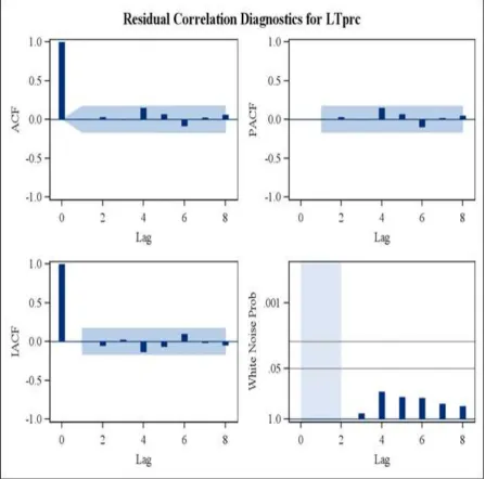
One last table (Table 4) checks for the autocorrelation check of residuals from the ARIMA (1, 1) model. Note that the check procedure referred to as the Ljung-Box (chi-square) statistics of 4.28, 8.96, 16.44,
and 17.91 for lags of 6, 12, 18 and 24. The p-values for these statistics are 0.3063, 0.4439, 0.4229 and 0.7113. None are significant at p-values less than or equal 0.05 or any other useful criterion. Hence, the ARIMA (1, 1) model satisfies the testing common to Box-Jenkins modeling methods. The autocorrelation function of the residual correlation diagnostics for the HK prices. Examine the histogram of residuals which appears close to “Normal” in Figures 3A and 3B.
Figure 3 (B):Normality diagnostics for HKPRC
Note, the similarity of the histogram of the residuals which appears close to normal in the plot. In addition, the QQ-Plot shows the observations approaching the 45 degree line indicating normality of the residuals.
Our last analysis concerns the index cross-correlation among exchanges for the closing prices of the Hong King (see Appendix A) denoted HKprc. The estimated intercept is 11.38068. Observe input numbers one through five. The overall regression factor for each are presented. None are very large and range from -0.06039 for NYvol to 0.02569 for lag HKvol. This indicates that the volume of the volume on the New York exchange does have some influence of closing prices on the Hong Kong exchange. This corroborates previous results previously observed.
Further Analysis of Results
In this study, we collected analyzed and interpreted an extensive data bank of stock market index numbers for the equity market of New York, London and Hong Kong and to a lesser extent for Singapore. The data analysis enabled us to draw conclusion concerning the association of these World markets. The analysis included an examination of the mean and volatility in the stock exchanges over a lengthy period of time and also study the relationships within sub-periods of the large length of time. We observed the rates of return and volatility of returns for the equity markets noting the differences in their rates of return and the volatility in
the rates of return. Observing that the means and volatility. Investigation into the mean and volatility of the rates of return bring to light the great difficulty in predicting mean and variation in rates of return as well as the volatility in these rates of return. In addition, the temporal analysis indicates the problems of prediction when one looks at the time series characteristics of the market indexes.
Jeffrey E Jarrett & Yifei Li | May 2016 | Vol.3| Issue 5|01-13 Tables 1, 2 and 3 in Appendix B do result
in very similar results.
To be consistent with the findings of CL, we observe only the H1, H3 and STI0 are significant (at α= to 0.05 or less) in 9a. In 9 b, the coefficients t-statistics are significant for H0 and STI0. Tables summarizing the relationships of the three markets may differ for the two or three predictor variables and the direction of the causality (i.e. signs of the coefficients). The differences in time periods should yield different results.
An additional question relates to whether or not there is a significant co-variation of volatility in a multivariate setting. To incorporate instantaneous causality in explaining Hang Seng volatility, one includes the current value of the variable in the other markets in the auto-regression. One observes the result for Hang Seng in column 2 of Appendix B Table 1 and the results in other markets in Appendix B Tables 2 and 3. The coefficients for the variables (all years) show some positive but only H2 and H3 are significant. This would indicate that the extended time period in this study results in some Hang Seng volatility being significant in period 1 for lag 1. A different interpretation of results just not indicated for other sub-time periods. Some may occur randomly and one has difficulty predicting pattern of consistency from period to period in pairwise combinations. Thus, we could conclude that the relationships among the markets change during the sub-periods indicating the dynamic aspects of capital markets studied. Volatility is present and changes the relationships of markets due to economic conditions, law affecting these markets, the growth of emerging markets versus more established markets. At hand, there is little doubt that market volatility is ever changing and the prediction of volatility not easily accomplished.
Without going through the analysis to compare individual coefficients, we observe the different effects of change in time and the pairwise relationship of markets. As long as economic conditions change, the results include temporal instabilities in markets.
Our study is lengthy and exhaustive butmuch of its results are not unnerving since we already know that markets vary in prices and volatility, but these factors have components that are predictable when using modern time series analysis. For example, see Ray, Chen and Jarrett (19970 where the authors demonstrate that firms listed on the Nikkei contain components (permanent and temporary) which may in turn lead to better predictions.
Observing Appendix B Table 2b, N1, N3, N4 and STI0 have estimated coefficients with significant t-statistics at αless than or equal to 0.05.This indicates that Nikkei has serial correlation at 1, 3 and 4 lags and contains one additional coefficient with STI0 at zero lag. In period 2, only STI0 contains a coefficient with a significant (t-statistics or p-value) at zero lag. The last sub-period (3), Nikkei contains significant coefficients at N1, H0 and ST0. Hence there no consistency in the three period.
In keeping with the exhaustive analysis, we observe the same lack of consistency in the analysis for Singapore. Lag STI2 contains a significant t-statistic for ST1 lagged values. H0 and N0 have significant t-statistics indicating and corroborating the observations before that Singapore, the smallest equity market is influenced by the larger Nikkei and Hang Sang exchanges. The three periods have different results. No one period is similar to each other and relationships over time will be influence by other factors.
Last, the results of the models for the volatility in equity returns for all the equity markets, we find the effect of the Asian equities leading to the same for temporal instability. Simply stated, the inclusion of the markets do not result in stable relationships throughout the three sub-periods. There are structural changes related to each time period. Hence, we conclude that the concept of temporal stability is not present which agrees with many previous studies done in earlier time periods.
Conclusions
for the equity markets of New York, Honk Kong and London. Our purpose is to draw conclusions concerning the relationship of the various equity markets expressed by an analysis of the mean and volatility in the stock exchanges over lengthy period of after defining three distinct sub-periods We first examining the time series characteristic of stock price indices for four exchanges during the period from 1987 until 2012 (we included the smaller Asian market of Singapore).
Specifically, we calculated the rate of return and volatility of returns for three major markets and estimated the serial correlation and co-movement of the equity markets. We found that the mean rates of return vary for the equity markets noting all have differences in their rates of return. Volatility in the rates of return also differ among the equity exchanges. Across the three sub-periods defined by time, the relationships among the markets are not stable. This, perhaps, is the most crucial of the general findings of the analysis and similar to JKK in a time series analysis of other stock markets. Relationship across equity markets change. Investigations into the influences of
the economic environment in which the markets operate would indicate what some of the causes and associations with the changes in the mean and variability of rates of return. Volatility in the rates of return would add to our knowledges of explaining and predicting relationships among equity markets. This evidence is consistent with other studies of Western and Asian markets.
Furthermore, we find that serial correlation also differs in the equity markets studied. The use of multivariate time series analysis (see Kuvita, [13]; Chen, Finney and Lai [14]; and Juselius, [15] may provide further evidence of the lack of co-integration in these stock exchanges. A more useful and better definition of temporal stability may add to the discussion of emerging markets of Asian and even the ones currently considered emerging. One earlier study noted before [16] suggests an alternative approach h using long memory time series modeling that both permanent and temporary components exist in the time series of Asian markets, i.e. the Japan equity market in their study [17-20].
References
1 Chow GC, Fan Z, Hu J (1999) Shanghai stock prices as determined by the present value model, Journal of Comparative Economics, 27:553-561.
2 Chen N (1991) Financial investment opportunities and the macro economy, The Journal of Finance, 46(2):529-554.
3 Cheung YW, Ng L (1998) International evidence on the stock market and aggregate economic activity, Journal of Empirical Finance, 5:281-296.
4 Liaw KT (2007) Investment Banking & Investment Opportunities in China: Comprehensive Guide for Finance Professionals John Wiley & Co.: New York 5 Fama E (1990) Stock returns, expected
returns, and real activity, Journal of Finance, 45:1089-1109.
6 Fama E (1991) Efficient Capital Markets: II. Journal of Finance, 46:1575-1617.
7 Wei K, Wong K (1992) Test of inflation and industry portfolio stock returns. Journal of Economics & Business, 44:77-94.
8 Zhong RS, Gu L, CB Lui (1999) the Empirical Statistical Analysis of Chinese Stock Markets, China Financial and Political Economics Press, Beijing.
9 Chow GC, Lawler CC (2003) A time series analysis of the Shanghai and New York stock price indices, Annals of Economics and Finance, 4:17-35.
10 Jarrett JE, Klein, AF, Kyper E (2013) Association between Asian Equity Markets and Western Markets: Evidence from the Indexes of Equity Markets. Asian Journal of Empirical Research, 3(8):972-989.
11 Jarrett JE, Sun T (2012) Association between the New York and Shanghai Markets: Evidence from the Stock Price Indices, Journal
of Business Economics and
Management,13(1):132-147.
Jeffrey E Jarrett & Yifei Li | May 2016 | Vol.3| Issue 5|01-13 13 Kuvita T (2010) Time Series Analysis of
Transatlantic Market Interactions: Evidence from Crude Oil and Gasoline Prices, International Journal of Business and Economics, 9:157-73.
14 Chen L, Finney M, Lai K S (2005) “A Threshold Cointegration of Asymmetric Price Transmission from Crude Oil to Gasoline Prices,” Econometrica Letters, 89:233-239. 15 Juselius K (2006) the Cointegrated VAR
Model: Methodology and Applications, Oxford University Press.
16 Ray B, Chen S, Jarrett JE (1997) Identifying permanent and temporary components in Japanese stock prices, Financial Engineering and the Japanese Markets, 4(3):233-256.
17 Bailey W, Cai J, Cheung F Wang (2009) Stock returns, order imbalances and commonality: Evidence on individual, institutional and proprietary investors in China, Journal of Finance, 45:1109-28.
18 Jarrett JE, Sun Z (2009A) Evidence and Explanations for the Association among Six Asian (Pacific-Basin) Financial Markets, Applied Economics, Vol. 41:25, 1-12.
19 Jarrett JE, Sun Z (2009B) Explaining Pacific-Basin Financial Market Returns by Size of Firm, International Review of Applied Financial Issues and Economics, 1:33-42.. 20 Pan X, Li K, Jarrett JE (2012) The
APPENDIX A
Index of Cross-correlation among exchanges
Model for variable LTprc
Estimated Intercept 9.952565
Autoregressive Factors
Factor 1: 1 - 1 B**(1)
Moving Average Factors
Factor 1: 1 + 0.04402 B**(1)
Input Number 1
Input Variable LTvol
Overall Regression Factor -0.04761
Input Number 2
Input Variable lagLTvol
Overall Regression Factor 0.032045
Input Number 3
Input Variable lag2LTvol
Overall Regression Factor 0.02401
Input Number 4
Input Variable HKvol
Overall Regression Factor -0.00078
Input Number 5
Input Variable NYvol
Overall Regression Factor -0.06015
APPENDIX A Volume Cross-correlation among exchanges (SAS Procedure Output)
Three HKvol LTvol
Variables NYvol
Descriptive Statistics
Variable N Mean Std. Dev. Sum Minimum Maximum
HKvol 152 0.9113 3129 3129 18.8681 22.0307
LTvol 135 0.3520 2829 2829 20.0979 21.4725
NYvol 158 20.774 3435 3435 20.7774 22.0370
Pearson Correlation Coefficients P-value (r) under Ho: ρ=0
Number of Coefficients
HKvol 1
52
-0.484 ≤.0000 1135
0.925 ≤.0000 152
LTvol -0.484
≤.0000 135
1.000
135 -.432 ≤.0000
Jeffrey E Jarrett & Yifei Li | May 2016 | Vol.3| Issue 5|01-13
NYvol .925
≤.0000 152
-0.432 ≤.0000 135
1.000 158
APPENDIX B
Table 1: Regressions of volatility of equity returns Hank Seng (Hong Kong)
All Years Pre1997 1997-2007 Post 2007
Constant
t 0.0072 0.0096 0.0078 0.0062
HO t H1
t 0.0181 0.6832 -0.0171 -0.3684 0.0575 1.3687 0.0293 0.5719
H2
t 0.0622 2.7874 0.1465 3.2980 0.0258 0.7399 0.0014 0.0399
H3
t 0.0570 2.5461 0.0744 1.6759 0.0470 1.3446 0.0463 1.2818
H4
t 0.0413 1.8323 0.0552 1.2415 0.0386 1.1003 0.0313 0.8674
N0
t 0.1144 4.3082 0.0119 0.2371 0.0903 1.9260 0.1851 4.7361
N1
t -0.0021 -0.0794 0.0146 0.2897 -0.0074 -0.1533 0.0265 0.6597
STI0
T 0.5356 20.9238 0.4056 6.7833 0.5290 14.7450 0.6705 14.4441
STI1
t 0.0148 0.5044 0.0060 0.0942 0.0229 0.5436 -0.0722 -1.2449
APPENDIX B
Table 2: Regressions of volatility of equity returns
Nikkei (Tokyo)
All Years Pre 1997 1997-2007 Post 2007
Constant t
0.0096 8.4516
0.0078 3.8930
0.0158 8.0776
.0081 3.8863
N0 T N1
T 0.1240 4.6691 0.1711 3.7345 0.0129 0.3004 0.1364 2.6559 N2
t 0.0447 1.7485 0.0724 1.5780 0.0521 1.2389 -0.0166 -0.3806 N3
t 0.0861 3.3705 0.1113 2.4201 0.0810 1.9249 0.0363 0.8347 N4
t 0.0256 1.0128 0.1796 3.8759 -0.0321 -0.7625 -0.0448 -1.0586 H0
T 0.1146 4.4347 0.0086 0.2077 0.0687 1.8344 0.2975 4.7029 H1
t -0.4201 -0.109 0.0234 .5659 -0.8204 -0.307 -0.0231 -0.3538 STI0
t 0.1937 6.8208 0.1440 2.5456 0.1150 3.0892 0.3517 4.9835 STI2
APPENDIX B
Table 3: Regressions of volatility or equity returns
STI (Singapore)
All Years Pre-1997 1997-2007 Post 2007
Constant
t -0.001 -0.617 0.005 2.675 -0.002 -.886 -0.002 -1.865 STI0
t STI1
t 0.098 3.695 0.077 1.616 0.077 1.844 0.167 3.277 STI2
t 0.082 3.652 0.123 2.730 0.026 0.762 0.160 4.415 STI3
t 0.079 3.482 0.046 1.022 0.073 2.084 0.086 2.356 STI4
t 0.086 3.814 0.045 0.987 0.120 3.381 -0.018 -0.504 H0
T 20.639 0.426 6.576 14.324 0.508 14.527 0.521 H1
t -0.016 -0.681 0.020 0.578 -0.019 -0.450 -0.060 -1.339 N0
t 0.151 6.371 0.100 2.722 0.138 2.973 0.155 4.529 N1