Vol 8, No 2 (2017)

Available online throug

ISSN 2229 – 5046

NONLINEAR RADIATION EFFECT

ON CASSON FLUID SATURATED NON-DARCY POROUS MEDIUM

N. VIJAYA, K. SREELAKSHMI* AND

G. SAROJAMMA

Department of Applied Mathematics,

Sri Padmavati Mahila Visvavidyalayam, Tirupati - 517502, India.

(Received On: 12-01-17; Revised & Accepted On: 01-02-17)

ABSTRACT

T

Keywords: Casson fluid, non-linear thermal radiation, non-Darcy porous medium, viscous dissipation.

1. INTRODUCTION

Study of non-Newtonian fluids is gaining importance due to its diverse range of applications in industry. Some examples of such fluids are lubricants, colloidal and suspension solutions, polymer solutions, fruit juice, paints etc. In non-Newtonian fluids, the relation between shear stress and shear rate is non-linear and hence, apparent viscosity of the fluid is not a constant. Various constitutive equations have been developed to describe a non-Newtonian fluid suitably. Casson fluid is one non-Newtonian fluid proposed by Casson to describe the flow curves of suspension of pigments in Lithographic varnishes used for printing inks. It is reported that this model described accurately the flow curves of suspensions of bentonite in water [1], suspension of Silicon [2] and several polymers [3] used in industry. Blood is also modeled as a Casson fluid as blood shows a Newtonian nature when it flows through larger diameter vessels and shows a highly non-Newtonian behavior while flowing through the smaller diameter vessels. Literature reveals that studies on heat and mass transfer in Casson fluid flows are very limited. Some of the researchers focused their study on these aspects in Casson fluids under different conditions [4–9].

Fluid flows over stretching surfaces have several industrial applications including extrusion of polymer or rubber sheets, glass blowing and continuous casting. In melt-spinning process, the extrudate from the die is drawn and stretched into a filament or sheet and is solidified by gradual cooling with water or chilled metal rolls. Heat transfer at the sheet has an important role on the quality of the final product. Extensive research has been done on stretching flows under different configurations.

Heat transfer in porous media plays a crucial role in different applications such as extraction of crude oil, thermal insulation and chemical reactors. Significant work has been reported on heat transfer in Darcy porous medium. Darcy law is valid when the flow rate is small. At higher rates of flow there is a variation from Darcy nature and non-Darcy nature prevails. The Darcy- Forchheimer model describes the effect of inertia as well as viscous forces in porous media. A detail review on heat transfer in Darcian and non-Darcian porous medium is found in Nield and Bejan [10].

Heat transfer in fluid flows over a stretching sheet due to thermal radiation has significant industrial applications in solar power technology, furnace design, solar ponds, heat exchangers, satellites and space vehicles. Recently, the concept of non-linear thermal radiative heat transfer has been introduced [11–13]. The presence of non-linear thermal radiation makes the energy equation strongly non-linear.

The objective of this analysis is to investigate the effect of non-linear thermal radiation and viscous heating on the MHD non-Darcy flow of an incompressible and electrically conducting Casson fluid induced due to a stretching surface.

2. MATHEMATICAL FORMULATION

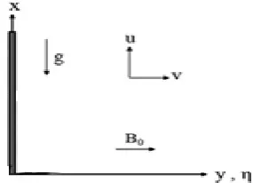
Consider the steady non-Darcy mixed convective heat and mass transfer of an incompressible and electrically conducting Casson fluid flow induced by a vertical stretching sheet embedded in a fluid saturated porous medium. A Cartesian coordinate system is taken with x-axis along the sheet and y-axis normal to the sheet as shown in Fig. 1. The flow region is subjected to a uniform transverse magnetic field 𝐵𝐵�⃗= (0,𝐵𝐵₀, 0) and uniform electric field 𝐸𝐸�⃗=

(0, 0,−𝐸𝐸0). It is assumed that the flow is generated by stretching of an elastic boundary sheet by imposing two equal

and opposite forces in such a way that velocity of the boundary sheet is of linear order of the flow direction. The Maxwell’s equations are ∇ ∙ 𝐵𝐵�⃗= 0 and ∇×𝐸𝐸�⃗= 0. From the Ohm’s law 𝐽𝐽⃗=σ ( 𝐸𝐸�⃗+ 𝑞𝑞⃗×𝐵𝐵�⃗), where 𝐽𝐽⃗ is the Joule current, 𝜎𝜎 is the magnetic permeability and 𝑞𝑞⃗ is the fluid velocity. The induced magnetic field due to the motion of the electrically conducting fluid is negligible. Temperature and species concentration are assumed to have quadratic variations with the distance from origin.

Fig. 1: Physical model and coordinate system

Constitutive equation of the Casson fluid can be written as

τ_ij =�

2�μ_B+ Py

√2π�eij, π > πc

2�μ_B+ Py

�2πc�eij , π < πc

(1)

where τ_ij is the (i, j)th component of the stress tensor, μ_B is the plastic dynamic viscosity of the non-Newtonian fluid,

Py is the yield stress of the fluid, π is the product of the component of deformation rate with itself, namely, π= eijeij,

and e_ij is the (i, j)th component of deformation rate, and π_c is the critical value of π based on the non-Newtonian model.

By applying boundary layer approximations, the governing equations are expressed as follows:

𝜕𝜕𝜕𝜕 𝜕𝜕𝜕𝜕+

𝜕𝜕𝜕𝜕

𝜕𝜕𝜕𝜕 = 0, (2) 1

𝜀𝜀2�𝜕𝜕

∂𝜕𝜕 ∂𝜕𝜕+𝜕𝜕

∂𝜕𝜕 ∂𝜕𝜕�=

𝜈𝜈 𝜀𝜀�1 +

1 𝛽𝛽�

∂2𝜕𝜕 ∂𝜕𝜕2+

𝜎𝜎

𝜌𝜌(𝐸𝐸0𝐵𝐵0− 𝐵𝐵02𝜕𝜕)− 𝜈𝜈 𝑘𝑘1𝜕𝜕 −

𝐶𝐶𝑏𝑏 �𝑘𝑘1𝜕𝜕

2_{, (3)}

𝜕𝜕∂_∂𝑇𝑇_𝜕𝜕+𝜕𝜕∂_∂𝑇𝑇_𝜕𝜕=_{𝜌𝜌𝐶𝐶}𝑘𝑘

𝑝𝑝 ∂2𝑇𝑇 ∂𝜕𝜕2+

16𝜎𝜎∗ 3𝑘𝑘∗_{𝜌𝜌𝑐𝑐𝑝𝑝}

𝜕𝜕 𝜕𝜕𝜕𝜕�𝑇𝑇3

𝜕𝜕𝑇𝑇 𝜕𝜕𝜕𝜕�+

𝜇𝜇 𝜌𝜌𝑐𝑐𝑝𝑝�1 +

1 𝛽𝛽� �

∂𝜕𝜕 ∂𝜕𝜕�

2

(4)

𝜕𝜕∂_∂𝐶𝐶_𝜕𝜕+𝜕𝜕∂_∂𝐶𝐶_𝜕𝜕=𝐷𝐷𝜕𝜕_∂2_𝜕𝜕𝐶𝐶2− 𝑘𝑘0(𝐶𝐶 − 𝐶𝐶∞), (5)

where u and v are the fluid velocity components along x and y axes, respectively,𝜀𝜀 is the porosity of the medium, 𝜈𝜈 is the kinematic viscosity, 𝜌𝜌 is the density of the fluid,𝐸𝐸₀ is the electric field strength in the transverse direction, 𝐵𝐵₀ is the transverse magnetic field strength,𝑘𝑘₁ is the permeability of porous medium, β= μ_B�2π_c /P_y is the Casson parameter,𝐶𝐶_𝑏𝑏 is the form of drag coefficient which is independent of viscosity and other physical properties of the fluid which depend on the geometry of the medium, 𝑇𝑇 is the temperature of the fluid inside the thermal boundary layer, 𝑇𝑇_𝑤𝑤 is the uniform temperature and 𝑇𝑇_∞ is the fluid temperature in the free stream with 𝑇𝑇_𝑤𝑤 >𝑇𝑇_∞, C is the fluid concentration,

𝐶𝐶𝑤𝑤 is the uniform concentration and 𝐶𝐶∞ is the fluid concentration in the free stream with 𝐶𝐶_𝑤𝑤>𝐶𝐶_∞, 𝑐𝑐_𝑝𝑝 is the specific heat at constant pressure, μis the dynamic viscosity of the fluid, 𝑘𝑘 is the thermal conductivity of the medium, 𝜎𝜎∗ is the Stefen-Boltzman constant and 𝑘𝑘∗ is the absorption coefficient, D is the mass diffusivity and 𝑘𝑘₀ is the chemical reaction. Boundary conditions are:

𝜕𝜕=𝜕𝜕𝑤𝑤(𝜕𝜕) +𝑁𝑁 �1 +_𝛽𝛽1� 𝜈𝜈𝜕𝜕𝜕𝜕_{𝜕𝜕𝜕𝜕} , 𝜕𝜕=𝜕𝜕𝑤𝑤, 𝑇𝑇= 𝑇𝑇𝑤𝑤 = 𝑇𝑇∞+ 𝐴𝐴0�𝜕𝜕_𝑙𝑙� 2

, 𝐶𝐶= 𝐶𝐶_𝑤𝑤 = 𝐶𝐶_∞+𝐴𝐴₁�𝜕𝜕

𝑙𝑙� 2

𝑎𝑎𝑎𝑎 𝜕𝜕= 0,

where 𝜕𝜕_𝑤𝑤(𝜕𝜕) =𝑏𝑏𝜕𝜕 is the velocity of the stretching surface, b is the proportionality constant of the stretching velocity,

𝐴𝐴0 and 𝐴𝐴1are the parameters of temperature and concentration distributions respectively on the stretching surface, is the

parameter of distribution on the stretching surface.

To solve the governing boundary layer equations (3) – (5), the following similarity transformations are introduced:

𝜕𝜕=𝑏𝑏𝜕𝜕𝑓𝑓′_{(𝜂𝜂),𝜕𝜕= −√𝑏𝑏𝜈𝜈𝑓𝑓(𝜂𝜂), 𝜂𝜂 =�}𝑏𝑏

𝜈𝜈𝜕𝜕 ,

𝜃𝜃(𝜂𝜂) = 𝑇𝑇−𝑇𝑇∞

𝑇𝑇𝑤𝑤−𝑇𝑇∞ , 𝜙𝜙(𝜂𝜂) = 𝐶𝐶−𝐶𝐶∞

𝐶𝐶𝑤𝑤−𝐶𝐶∞ (7)

Substitution of equation (7) into the governing equations (3) – (5) and using the above relations we finally obtain a system of non-linear ordinary differential equations

�1 +_𝛽𝛽1�𝑓𝑓_𝜀𝜀′′′+𝑓𝑓𝑓𝑓_𝜀𝜀2′′−

𝑓𝑓′2

𝜀𝜀2+𝑀𝑀2(𝐸𝐸1− 𝑓𝑓

′_{)− 𝐹𝐹}∗_𝑓𝑓′2

− 𝑘𝑘𝑝𝑝𝑓𝑓′ =0, (8)

𝜃𝜃′′_{+𝑁𝑁𝑁𝑁[(1 + (𝜃𝜃}

𝑤𝑤−1)𝜃𝜃)3]𝜃𝜃′′+ 3𝑁𝑁𝑁𝑁[(𝜃𝜃𝑤𝑤−1)(1 + (𝜃𝜃𝑤𝑤−1)𝜃𝜃)2]𝜃𝜃′2

+𝑃𝑃𝑁𝑁 �𝑓𝑓𝜃𝜃′−2𝑓𝑓′𝜃𝜃+𝐸𝐸𝑐𝑐 �1 +1 𝛽𝛽�(𝑓𝑓′′)

2_{�=0, (9)}

𝜙𝜙′′_{+𝑆𝑆𝑐𝑐(𝑓𝑓𝜙𝜙′−2𝑓𝑓}′_{𝜙𝜙 − 𝛾𝛾𝜙𝜙) =0, (10)}

Boundary conditions (6) reduce to:

𝑓𝑓(0) = 0, 𝑓𝑓′(0) =1,𝜃𝜃(0) = 1, 𝜙𝜙(0) = 1 𝑎𝑎𝑎𝑎 𝜂𝜂=0, (11)

𝑓𝑓′(∞) =0, 𝜃𝜃(∞) =0, 𝜙𝜙(∞) =0 𝑎𝑎𝑎𝑎 𝜂𝜂→∞, (12) where primes denote differentiation with respect to 𝜂𝜂, 𝑀𝑀2= 𝜎𝜎𝐵𝐵₀2_{⁄𝜌𝜌𝑏𝑏is magnetic parameter, 𝑘𝑘}

𝑝𝑝 =𝜈𝜈 𝑘𝑘⁄ 1𝑏𝑏 is porous

parameter, 𝐸𝐸1=𝐸𝐸0⁄𝐵𝐵0𝑏𝑏𝜕𝜕 is electric field parameter,𝐹𝐹∗=𝐶𝐶𝑏𝑏𝜕𝜕

�𝑘𝑘1 is inertial parameter, 𝑃𝑃𝑁𝑁=𝜌𝜌𝑐𝑐𝑝𝑝𝜈𝜈 𝑘𝑘⁄ is Prandtl number,

𝑁𝑁𝑁𝑁= 16𝜎𝜎∗_𝑇𝑇∞3_{⁄3𝑘𝑘𝑘𝑘∗ is thermal radiation parameter, 𝜃𝜃}

𝑤𝑤= Tw⁄ T∞ is temperature ratio parameter,𝐸𝐸𝑐𝑐= 𝑏𝑏2𝑙𝑙2�𝑐𝑐𝑝𝑝𝐴𝐴0 is Eckert number, 𝑆𝑆𝑐𝑐=𝜈𝜈 𝐷𝐷⁄ is Schmidt number, 𝛾𝛾=𝑘𝑘₀⁄𝑏𝑏 is chemical reaction parameter.

The Physical quantities of engineering interest in this problem are the skin friction coefficient 𝐶𝐶_𝑓𝑓, Nusselt number 𝑁𝑁𝜕𝜕_𝜕𝜕 and Sherwood number 𝑆𝑆ℎ_𝜕𝜕. The skin friction coefficient 𝐶𝐶_𝑓𝑓, is defined by

𝐶𝐶𝑓𝑓= _{𝜌𝜌𝜕𝜕}2𝜏𝜏𝑤𝑤_𝑤𝑤2, (13)

where the wall shear stress 𝜏𝜏_𝑤𝑤 is given by

𝜏𝜏𝑤𝑤 =𝜇𝜇 �𝜕𝜕𝜕𝜕_{𝜕𝜕𝜕𝜕}�

𝜕𝜕=0

. (14)

Using the non-dimensional variables equation (7), we get from equations (13) and (14) as 1

2𝐶𝐶𝑓𝑓�𝑅𝑅𝑒𝑒𝜕𝜕=�1 +

1

𝛽𝛽� 𝑓𝑓′′(0). (15)

The local Nusselt number which is defined as

𝑁𝑁𝜕𝜕𝜕𝜕= _𝐾𝐾(𝜕𝜕_{𝑇𝑇𝑤𝑤}𝑞𝑞_−𝑇𝑇𝑤𝑤_∞), (16)

where 𝑞𝑞_𝑤𝑤is the heat transfer from the sheet is given by

𝑞𝑞𝑤𝑤 = −𝐾𝐾 �𝜕𝜕𝑇𝑇_{𝜕𝜕𝜕𝜕}�

𝜕𝜕=0. (17)

Using the non-dimensional variables (7), we get from equations (16) and (17) as

𝑁𝑁𝜕𝜕𝜕𝜕/𝑅𝑅𝑒𝑒𝜕𝜕1/2= −(1 +𝑁𝑁𝑁𝑁𝜃𝜃𝑤𝑤3)𝜃𝜃′(0). (18)

The local Sherwood number is defined by

𝑆𝑆ℎ𝜕𝜕= _{𝐷𝐷𝑚𝑚(}𝜕𝜕𝑞𝑞_{𝐶𝐶𝑤𝑤}𝑚𝑚_{−𝐶𝐶∞)}, (19)

where 𝑞𝑞_𝑚𝑚 is the mass transfer which is defined by

𝑞𝑞𝑚𝑚 = −𝐷𝐷𝑚𝑚�𝜕𝜕𝐶𝐶_{𝜕𝜕𝜕𝜕}�

𝜕𝜕=0, (20)

Using the non-dimensional variables (7), we get from (19) and (20) as

𝑆𝑆ℎ𝜕𝜕/𝑅𝑅𝑒𝑒𝜕𝜕1/2= −𝜙𝜙′(0). (21)

where 𝑅𝑅𝑒𝑒_𝜕𝜕 = 𝜕𝜕𝑤𝑤𝜕𝜕

3. METHOD OF SOLUTION

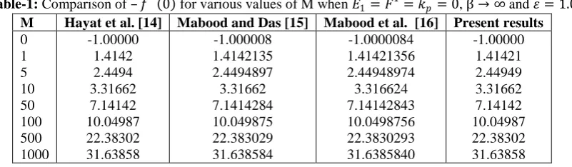
Equations (8) – (12) together with the boundary conditions are solved numerically using the Runge-Kutta fifth order method along with shooting technique. To ensure the accuracy of the numerical method, results of the present analysis are compared with those of Hayat et al. [14], Mabood and Das [15], Mabood et al. [16] in the absence of 𝐸𝐸₁=𝐹𝐹∗=

𝑘𝑘𝑝𝑝= 0, and 𝜀𝜀= 1.0 in case of Newtonian fluid for different values of M. Table 1 shows that the results are in good

agreement.

Table-1: Comparison of –𝑓𝑓′′(0) for various values of M when 𝐸𝐸₁=𝐹𝐹∗=𝑘𝑘_𝑝𝑝= 0,β → ∞and 𝜀𝜀= 1.0

M Hayat et al. [14] Mabood and Das [15] Mabood et al. [16] Present results

0 1 5 10 50 100 500 1000

-1.00000 1.4142 2.4494 3.31662 7.14142 10.04987 22.38302 31.63858

-1.000008 1.4142135 2.4494897 3.31662 7.1414284 10.049875 22.383029 31.638584

-1.0000084 1.41421356 2.44948974 3.316624 7.14142843 10.0498756 22.3830293 31.6385840

-1.00000 1.41421 2.44949 3.31662 7.14142 10.04987 22.38302 31.63858

4. RESULTS AND DISCUSSION

In this analysis numerical solutions are obtained to investigate the effect of various governing parameters on non-Darcy flow over a stretching surface in the presence of a magnetic field, electrical field, non-linear thermal radiation, viscous dissipation and chemical reaction. The computational results are shown through graphs and discussed.

Fig. 2 reveals that the velocity decreases throughout the boundary layer region which leads to thinning of the boundary layers for increasing values of Casson parameter(β). The temperature and concentration increase with increasing values of β as illustrated in Figs. 3 and 4. The corresponding thermal and solutal boundary layers become thicker. Fig. 5 shows that the effect of magnetic parameter is to diminish the velocity distribution in the boundary layer leading to thinning of the boundary layer. This is due to the Lorentz force developed due to the transverse magnetic field, which resists the fluid motion. As a result temperature and concentration of the fluid are seen to increase with increase in M (Figs. 6 and 7) and the thickness of the associated thermal and solutal boundary layers is increased.

The variation of porosity parameter (𝜀𝜀) of porous medium is plotted in Figs. 8 – 10. For an increase in the value of the porosity parameter, velocity distribution in the fluid flow increases whereas temperature and concentration are seen to decrease. Figs. 11 – 13 depict the influence of inertial parameter (𝐹𝐹∗) on the velocity, temperature and concentration. It is clear from Fig. 14 that the velocity gets diminished with increase in the value of F* while a reversal trend in temperature and concentration is found. Fig. 14 illustrates that electric parameter (𝐸𝐸₁) increases the velocity distribution throughout the hydrodynamic boundary layer in the vicinity of the boundary. However, a little away from the stretching sheet, the enhancement in velocity is more pronounced. Fig. 15 shows that temperature is dropped for an increase in electric field parameter due to increase in the mass flux. Species concentration shows a reduction for an increase in 𝐸𝐸₁ (Fig. 16). Fig. 17 indicates that velocity distribution shows a decreasing tendency with increasing values of porous permeability parameter(𝑘𝑘_𝑝𝑝), as expected and consequently the temperature and concentration distributions are increased (Figs. 18 and 19).

Fig. 20 depicts that the temperature is a decreasing function of Prandtl number (Pr) in the thermal boundary layer. For higher Prandtl number fluids, the thermal diffusivity is smaller. Hence, increasing values of Prandtl number result in decrease in the temperature. Fig. 21 shows that larger values of Nr imply enhanced radiation which leads to increase in temperature. From Fig. 22 it is clear that the variation of temperature ratio parameter (𝜃𝜃_𝑤𝑤) is similar to that of the radiation parameter. Fig. 23 depicts that increased values of Eckert number (Ec) enhance the temperature due to release of energy due to frictional heating and hence temperature raises. When Ec assumes values greater than 0.7, an over shoot above the prescribed value of the surface temperature occurs on the boundary.

Figure-2: Velocity profiles for different Values of 𝛽𝛽

Figure-3: Temperature profiles for different values of 𝛽𝛽

Figure-4: Concentration profiles for different values of 𝛽𝛽

0 1 2 3 4 5 6 7 8

0 0.1 0.2 0.3 0.4 0.5 0.6 0.7 0.8 0.9 1

η

f '

(η

) _{M = 2.0; ε = 1.2; E}

1 = 0.01; F * _{= k}

p = 0.1; Pr = 2.5; Nr = 0.5; θ

w = 1.1; Ec = 0.2; Sc = 1.2; γ = 0.1 M = 2.0; ε = 1.2; E₁ = 0.01; F* = k_p = 0.1; Pr = 2.5; Nr = 0.5; θ

w = 1.1; Ec = 0.2; Sc = 1.2; γ = 0.1 M = 2.0; ε = 1.2; E₁ = 0.01; F* = k_p = 0.1; Pr = 2.5; Nr = 0.5; θ

w = 1.1; Ec = 0.2; Sc = 1.2; γ = 0.1 M = 2.0; ε = 1.2; E₁ = 0.01; F* = k_p = 0.1; Pr = 2.5; Nr = 0.5; θ

w = 1.1; Ec = 0.2; Sc = 1.2; γ = 0.1

β = 0.5

β = 1.0

β = 1.5

β = 2.0

0 1 2 3 4 5 6 7 8

0 0.1 0.2 0.3 0.4 0.5 0.6 0.7 0.8 0.9 1

η

θ

(η

) M = 2.0; ε = 1.2; E₁ = 0.01; F* = k_p = 0.1; Pr = 2.5; Nr = 0.5; θ_w = 1.1; Ec = 0.2; Sc = 1.2; γ = 0.1 M = 2.0; ε = 1.2; E₁ = 0.01; F* = k_p = 0.1; Pr = 2.5; Nr = 0.5; θ_w = 1.1; Ec = 0.2; Sc = 1.2; γ = 0.1 M = 2.0; ε = 1.2; E₁ = 0.01; F* = k_p = 0.1; Pr = 2.5; Nr = 0.5; θ_w = 1.1; Ec = 0.2; Sc = 1.2; γ = 0.1 M = 2.0; ε = 1.2; E₁ = 0.01; F* = k_p = 0.1; Pr = 2.5; Nr = 0.5; θ_w = 1.1; Ec = 0.2; Sc = 1.2; γ = 0.1

β = 0.5

β = 1.0

β = 1.5

β = 2.0

0 1 2 3 4 5 6 7 8

0 0.1 0.2 0.3 0.4 0.5 0.6 0.7 0.8 0.9 1

η

φ

(η

) M = 2.0; ε = 1.2; E₁ = 0.01; F* = k_p = 0.1; Pr = 2.5; Nr = 0.5; θ_w = 1.1; Ec = 0.2; Sc = 1.2; γ = 0.1 M = 2.0; ε = 1.2; E₁ = 0.01; F* = k_p = 0.1; Pr = 2.5; Nr = 0.5; θ_w = 1.1; Ec = 0.2; Sc = 1.2; γ = 0.1 M = 2.0; ε = 1.2; E₁ = 0.01; F* = k_p = 0.1; Pr = 2.5; Nr = 0.5; θ_w = 1.1; Ec = 0.2; Sc = 1.2; γ = 0.1 M = 2.0; ε = 1.2; E₁ = 0.01; F* = k_p = 0.1; Pr = 2.5; Nr = 0.5; θ_w = 1.1; Ec = 0.2; Sc = 1.2; γ = 0.1

β = 0.5

β = 1.0

β = 1.5

Figure-5: Velocity profiles for different Values of M

Figure-6: Temperature profiles for different values of M

Figure-7: Concentration profiles for different values of M

0 1 2 3 4 5 6 7 8

0 0.1 0.2 0.3 0.4 0.5 0.6 0.7 0.8 0.9 1

η

f '

(η

) _{β = 0.5; ε = 1.2; E}

1 = 0.01; F *

= k_p = 0.1; Pr = 2.5; Nr = 0.5; θ_w = 1.1; Ec = 0.2; Sc = 1.2; γ = 0.1 β = 0.5; ε = 1.2; E₁ = 0.01; F* = k_p = 0.1; Pr = 2.5; Nr = 0.5; θ_w = 1.1; Ec = 0.2; Sc = 1.2; γ = 0.1 β = 0.5; ε = 1.2; E₁ = 0.01; F* = k_p = 0.1; Pr = 2.5; Nr = 0.5; θ_w = 1.1; Ec = 0.2; Sc = 1.2; γ = 0.1 β = 0.5; ε = 1.2; E₁ = 0.01; F* = k_p = 0.1; Pr = 2.5; Nr = 0.5; θ_w = 1.1; Ec = 0.2; Sc = 1.2; γ = 0.1

M = 2.0 M = 3.0 M = 4.0 M = 5.0

0 1 2 3 4 5 6 7 8

0 0.1 0.2 0.3 0.4 0.5 0.6 0.7 0.8 0.9 1

η

θ

(η

) β = 0.5; ε = 1.2; E

1 = 0.01; F * _{= k}

p = 0.1; Pr = 2.5;

Nr = 0.5; θ_w = 1.1; Ec = 0.2; Sc = 1.2; γ = 0.1 β = 0.5; ε = 1.2; E

1 = 0.01; F * _{= k}

p = 0.1; Pr = 2.5;

Nr = 0.5; θ_w = 1.1; Ec = 0.2; Sc = 1.2; γ = 0.1 β = 0.5; ε = 1.2; E

1 = 0.01; F * _{= k}

p = 0.1; Pr = 2.5;

Nr = 0.5; θ_w = 1.1; Ec = 0.2; Sc = 1.2; γ = 0.1 β = 0.5; ε = 1.2; E

1 = 0.01; F * _{= k}

p = 0.1; Pr = 2.5;

Nr = 0.5; θ_w = 1.1; Ec = 0.2; Sc = 1.2; γ = 0.1 M = 2.0 M = 3.0 M = 4.0 M = 5.0

0 1 2 3 4 5 6 7 8

0 0.1 0.2 0.3 0.4 0.5 0.6 0.7 0.8 0.9 1

η

φ

(η

) β = 0.5; ε = 1.2; E

1 = 0.01; F * _{= k}

p = 0.1; Pr = 2.5; Nr = 0.5; θ_w = 1.1; Ec = 0.2; Sc = 1.2; γ = 0.1 β = 0.5; ε = 1.2; E

1 = 0.01; F * _{= k}

p = 0.1; Pr = 2.5; Nr = 0.5; θ_w = 1.1; Ec = 0.2; Sc = 1.2; γ = 0.1 β = 0.5; ε = 1.2; E

1 = 0.01; F * _{= k}

p = 0.1; Pr = 2.5; Nr = 0.5; θ_w = 1.1; Ec = 0.2; Sc = 1.2; γ = 0.1 β = 0.5; ε = 1.2; E

1 = 0.01; F * _{= k}

p = 0.1; Pr = 2.5; Nr = 0.5; θ_w = 1.1; Ec = 0.2; Sc = 1.2; γ = 0.1

Figure-8: Velocity profiles for different Values of 𝜀𝜀

Figure-9: Temperature profiles for different values of 𝜀𝜀

Figure-10: Concentration profiles for different values of 𝜀𝜀

0 1 2 3 4 5 6 7 8

0 0.1 0.2 0.3 0.4 0.5 0.6 0.7 0.8 0.9 1

η

f '

(η

) _{β = 0.5; M = 2.0; E}

1 = 0.01; F * _{= k}

p = 0.1; Pr = 2.5; Nr = 0.5; θ_w = 1.1; Ec = 0.2; Sc = 1.2; γ = 0.1 β = 0.5; M = 2.0; E₁ = 0.01; F* = k_p = 0.1; Pr = 2.5; Nr = 0.5; θ_w = 1.1; Ec = 0.2; Sc = 1.2; γ = 0.1 β = 0.5; M = 2.0; E₁ = 0.01; F* = k_p = 0.1; Pr = 2.5; Nr = 0.5; θ_w = 1.1; Ec = 0.2; Sc = 1.2; γ = 0.1 β = 0.5; M = 2.0; E₁ = 0.01; F* = k_p = 0.1; Pr = 2.5; Nr = 0.5; θ_w = 1.1; Ec = 0.2; Sc = 1.2; γ = 0.1

ε = 1.2

ε = 1.8

ε = 2.2

ε = 2.8

0 1 2 3 4 5 6 7 8

0 0.1 0.2 0.3 0.4 0.5 0.6 0.7 0.8 0.9 1

η

θ

(η

) β = 0.5; M = 2.0; E₁ = 0.01; F* = k_p = 0.1; Pr = 2.5; Nr = 0.5; θ_w = 1.1; Ec = 0.2; Sc = 1.2; γ = 0.1 β = 0.5; M = 2.0; E₁ = 0.01; F* = k_p = 0.1; Pr = 2.5; Nr = 0.5; θ_w = 1.1; Ec = 0.2; Sc = 1.2; γ = 0.1 β = 0.5; M = 2.0; E₁ = 0.01; F* = k_p = 0.1; Pr = 2.5; Nr = 0.5; θ_w = 1.1; Ec = 0.2; Sc = 1.2; γ = 0.1 β = 0.5; M = 2.0; E₁ = 0.01; F* = k_p = 0.1; Pr = 2.5; Nr = 0.5; θ_w = 1.1; Ec = 0.2; Sc = 1.2; γ = 0.1

ε = 1.2

ε = 1.8

ε = 2.2

ε = 2.8

0 1 2 3 4 5 6 7 8

0 0.1 0.2 0.3 0.4 0.5 0.6 0.7 0.8 0.9 1

η

φ

(η

) β = 0.5; M = 2.0; E

1 = 0.01; F * _{= k}

p = 0.1; Pr = 2.5; Nr = 0.5; θ

w = 1.1; Ec = 0.2; Sc = 1.2; γ = 0.1 β = 0.5; M = 2.0; E

1 = 0.01; F * _{= k}

p = 0.1; Pr = 2.5; Nr = 0.5; θ

w = 1.1; Ec = 0.2; Sc = 1.2; γ = 0.1 β = 0.5; M = 2.0; E

1 = 0.01; F * _{= k}

p = 0.1; Pr = 2.5; Nr = 0.5; θ

w = 1.1; Ec = 0.2; Sc = 1.2; γ = 0.1 β = 0.5; M = 2.0; E

1 = 0.01; F * _{= k}

p = 0.1; Pr = 2.5; Nr = 0.5; θ

w = 1.1; Ec = 0.2; Sc = 1.2; γ = 0.1

ε = 1.2

ε = 1.8

ε = 2.2

Figure-11: Velocity profiles for different Values of 𝐹𝐹∗

Figure-12: Temperature profiles for different values of 𝐹𝐹∗

Figure-13: Concentration profiles for different values of 𝐹𝐹∗

0 1 2 3 4 5 6 7

0 0.1 0.2 0.3 0.4 0.5 0.6 0.7 0.8 0.9 1

η

f '

(η

) β = 0.5; M = 1.0; ε = 1.2; E1 = 0.01; kp = 0.1; Pr = 2.5; Nr = 0.5; θ_w = 1.1; Ec = 0.2; Sc = 1.2; γ = 0.1

F* = 1.0

F* = 2.0 F* = 3.0

F* = 4.0

0 0.5 1 1.5 2 2.5 3 3.5 4 4.5 5 0

0.1 0.2 0.3 0.4 0.5 0.6 0.7 0.8 0.9 1

η

θ

(η

) β = 0.5; M = 1.0; ε = 1.2; E1 = 0.01; kp = 0.1; Pr = 2.5; Nr = 0.5; θ_w = 1.1; Ec = 0.2; Sc = 1.2; γ = 0.1

F* = 1.0

F* = 2.0

F* = 3.0

F* = 4.0

0 0.5 1 1.5 2 2.5 3 3.5 4 4.5 5 0

0.1 0.2 0.3 0.4 0.5 0.6 0.7 0.8 0.9 1

η

φ

(η

) β = 0.5; M = 1.0; ε = 1.2; E₁ = 0.01; k_p = 0.1; Pr = 2.5; Nr = 0.5; θ_w = 1.1; Ec = 0.2; Sc = 1.2; γ = 0.1

F* = 1.0

F* = 2.0

F* = 3.0

Figure-14: Velocity profiles for different Values of 𝐸𝐸₁

Figure-15: Temperature profiles for different values of 𝐸𝐸₁

Figure-16: Concentration profiles for different values of 𝐸𝐸₁

0 1 2 3 4 5 6 7 8

0 0.1 0.2 0.3 0.4 0.5 0.6 0.7 0.8 0.9 1

η

f '

(η

) _{β = 0.5; M = 2.0; ε = 1.2; F}* _{= k}

p = 0.1; Pr = 2.5;

Nr = 0.5; θ_w = 1.1; Ec = 0.2; Sc = 1.2; γ = 0.1 β = 0.5; M = 2.0; ε = 1.2; F* = k

p = 0.1; Pr = 2.5;

Nr = 0.5; θ_w = 1.1; Ec = 0.2; Sc = 1.2; γ = 0.1 β = 0.5; M = 2.0; ε = 1.2; F* = k

p = 0.1; Pr = 2.5;

Nr = 0.5; θ_w = 1.1; Ec = 0.2; Sc = 1.2; γ = 0.1 β = 0.5; M = 2.0; ε = 1.2; F* = k

p = 0.1; Pr = 2.5;

Nr = 0.5; θ_w = 1.1; Ec = 0.2; Sc = 1.2; γ = 0.1

E₁ = 0.01

E₁ = 0.04

E

1 = 0.07

E

1 = 0.1

0 1 2 3 4 5 6

0 0.1 0.2 0.3 0.4 0.5 0.6 0.7 0.8 0.9 1

η

θ

(η

) β = 0.5; M = 2.0; ε = 1.2; F* = k_p = 0.1; Pr = 2.5; Nr = 0.5; θ

w = 1.1; Ec = 0.2; Sc = 1.2; γ = 0.1 β = 0.5; M = 2.0; ε = 1.2; F* = k_p = 0.1; Pr = 2.5; Nr = 0.5; θ

w = 1.1; Ec = 0.2; Sc = 1.2; γ = 0.1 β = 0.5; M = 2.0; ε = 1.2; F* = k_p = 0.1; Pr = 2.5; Nr = 0.5; θ

w = 1.1; Ec = 0.2; Sc = 1.2; γ = 0.1 β = 0.5; M = 2.0; ε = 1.2; F* = k_p = 0.1; Pr = 2.5; Nr = 0.5; θ

w = 1.1; Ec = 0.2; Sc = 1.2; γ = 0.1 E₁ = 0.01

E₁ = 0.04

E₁ = 0.07

E₁ = 0.1

0 1 2 3 4 5 6

0 0.1 0.2 0.3 0.4 0.5 0.6 0.7 0.8 0.9 1

η

φ

(η

) β = 0.5; M = 2.0; ε = 1.2; F* = k_p = 0.1; Pr = 2.5; Nr = 0.5; θ_w = 1.1; Ec = 0.2; Sc = 1.2; γ = 0.1 β = 0.5; M = 2.0; ε = 1.2; F* = k_p = 0.1; Pr = 2.5; Nr = 0.5; θ_w = 1.1; Ec = 0.2; Sc = 1.2; γ = 0.1 β = 0.5; M = 2.0; ε = 1.2; F* = k_p = 0.1; Pr = 2.5; Nr = 0.5; θ_w = 1.1; Ec = 0.2; Sc = 1.2; γ = 0.1 β = 0.5; M = 2.0; ε = 1.2; F* = k_p = 0.1; Pr = 2.5; Nr = 0.5; θ_w = 1.1; Ec = 0.2; Sc = 1.2; γ = 0.1

E₁ = 0.01

E₁ = 0.04

E₁ = 0.07

Figure-17: Velocity profiles for different Values of 𝑘𝑘_𝑝𝑝

Figure-18: Temperature profiles for different values of 𝑘𝑘_𝑝𝑝

Figure-19: Concentration profiles for different values of 𝑘𝑘_𝑝𝑝

0 1 2 3 4 5 6 7 8

0 0.1 0.2 0.3 0.4 0.5 0.6 0.7 0.8 0.9 1

η

f '

(η

) _{β = 0.5; M = 2.0; ε = 1.2; E}

1 = 0.01; F *

= 0.1; Pr = 1.0; Nr = 0.5; θ_w = 1.1; Ec = 0.2; Sc = 0.8; γ = 0.1

β = 0.5; M = 2.0; ε = 1.2; E₁ = 0.01; F* = 0.1; Pr = 1.0; Nr = 0.5; θ_w = 1.1; Ec = 0.2; Sc = 0.8; γ = 0.1

β = 0.5; M = 2.0; ε = 1.2; E₁ = 0.01; F* = 0.1; Pr = 1.0; Nr = 0.5; θ_w = 1.1; Ec = 0.2; Sc = 0.8; γ = 0.1

β = 0.5; M = 2.0; ε = 1.2; E₁ = 0.01; F* = 0.1; Pr = 1.0; Nr = 0.5; θ_w = 1.1; Ec = 0.2; Sc = 0.8; γ = 0.1

k_p = 0.1

k_p = 0.5

k_p = 1.0

k_p = 1.5

0 1 2 3 4 5 6 7 8

0 0.1 0.2 0.3 0.4 0.5 0.6 0.7 0.8 0.9 1

η

θ

(η

) β = 0.5; M = 2.0; ε = 1.2; E₁ = 0.01; F* = 0.1; Pr = 1.0; Nr = 0.5; θ_w = 1.1; Ec = 0.2; Sc = 0.8; γ = 0.1

k_p = 0.1

k_p = 0.5

k_p = 1.0

k_p = 1.5

0 1 2 3 4 5 6 7 8

0 0.1 0.2 0.3 0.4 0.5 0.6 0.7 0.8 0.9 1

η

φ

(η

) β = 0.5; M = 2.0; ε = 1.2; E₁ = 0.01; F* = 0.1; Pr = 1.0; Nr = 0.5; θ_w = 1.1; Ec = 0.2; Sc = 0.8; γ = 0.1

β = 0.5; M = 2.0; ε = 1.2; E₁ = 0.01; F* = 0.1; Pr = 1.0; Nr = 0.5; θ_w = 1.1; Ec = 0.2; Sc = 0.8; γ = 0.1

β = 0.5; M = 2.0; ε = 1.2; E₁ = 0.01; F* = 0.1; Pr = 1.0; Nr = 0.5; θ_w = 1.1; Ec = 0.2; Sc = 0.8; γ = 0.1

β = 0.5; M = 2.0; ε = 1.2; E₁ = 0.01; F* = 0.1; Pr = 1.0; Nr = 0.5; θ_w = 1.1; Ec = 0.2; Sc = 0.8; γ = 0.1

k_p = 0.1

k_p = 0.5

k_p = 1.0

k

Figure-20: Temperature profiles for different values of Pr

Figure-21: Temperature profiles for different values of Nr

Figure-22: Temperature profiles for different values of 𝜃𝜃_𝑤𝑤

0 2 4 6 8 10 12

0 0.1 0.2 0.3 0.4 0.5 0.6 0.7 0.8 0.9 1

η

θ

(η

) β = 0.5; M = 2.0; ε = 1.2; E₁ = 0.01; F* = k_p = 0.1; Nr = 0.5; θ_w = 1.1; Ec = 0.2; Sc = 1.2; γ = 0.1 β = 0.5; M = 2.0; ε = 1.2; E₁ = 0.01; F* = k_p = 0.1; Nr = 0.5; θ_w = 1.1; Ec = 0.2; Sc = 1.2; γ = 0.1 β = 0.5; M = 2.0; ε = 1.2; E₁ = 0.01; F* = k_p = 0.1; Nr = 0.5; θ_w = 1.1; Ec = 0.2; Sc = 1.2; γ = 0.1 β = 0.5; M = 2.0; ε = 1.2; E₁ = 0.01; F* = k_p = 0.1; Nr = 0.5; θ_w = 1.1; Ec = 0.2; Sc = 1.2; γ = 0.1

Pr = 0.7 Pr = 1.0 Pr = 2.0 Pr = 3.0

0 1 2 3 4 5 6 7 8 9 10

0 0.1 0.2 0.3 0.4 0.5 0.6 0.7 0.8 0.9 1

η

θ

(η

) β = 0.5; M = 2.0; ε = 1.2; E₁ = 0.01; F* = k_p = 0.1; Pr = 2.5; θ_w = 1.1; Ec = 0.2; Sc = 1.2; γ = 0.1 β = 0.5; M = 2.0; ε = 1.2; E₁ = 0.01; F* = k_p = 0.1; Pr = 2.5; θ_w = 1.1; Ec = 0.2; Sc = 1.2; γ = 0.1 β = 0.5; M = 2.0; ε = 1.2; E₁ = 0.01; F* = k_p = 0.1; Pr = 2.5; θ_w = 1.1; Ec = 0.2; Sc = 1.2; γ = 0.1 β = 0.5; M = 2.0; ε = 1.2; E₁ = 0.01; F* = k_p = 0.1; Pr = 2.5; θ_w = 1.1; Ec = 0.2; Sc = 1.2; γ = 0.1

Nr = 0.5 Nr = 1.0 Nr = 1.5 Nr = 2.0

0 1 2 3 4 5 6 7 8

0 0.1 0.2 0.3 0.4 0.5 0.6 0.7 0.8 0.9 1

η

θ

(η

) β = 0.5; M = 2.0; ε = 1.2; E₁ = 0.01; F* = k_p = 0.1;

Pr = 2.5; Nr = 0.5; Ec = 0.2; Sc = 1.2; γ = 0.1 β = 0.5; M = 2.0; ε = 1.2; E₁ = 0.01; F* = k_p = 0.1; Pr = 2.5; Nr = 0.5; Ec = 0.2; Sc = 1.2; γ = 0.1 β = 0.5; M = 2.0; ε = 1.2; E₁ = 0.01; F* = k_p = 0.1; Pr = 2.5; Nr = 0.5; Ec = 0.2; Sc = 1.2; γ = 0.1 β = 0.5; M = 2.0; ε = 1.2; E₁ = 0.01; F* = k_p = 0.1; Pr = 2.5; Nr = 0.5; Ec = 0.2; Sc = 1.2; γ = 0.1

θ_w = 1.1

θ_w = 1.4

θ_w = 1.7

Figure-23: Temperature profiles for different values of Ec

Figure-24: Concentration profiles for different values of Sc

Figure-25: Concentration profiles for different values of 𝛾𝛾

0 1 2 3 4 5 6 7 8

0 0.2 0.4 0.6 0.8 1

η

θ

(η

)

β = 0.5; M = 2.0; ε = 1.2; E

1 = 0.01; F * _{= k}

p = 0.1; Pr = 2.5; Nr = 0.5; θ

w = 1.1; Sc = 1.2; γ = 0.1 β = 0.5; M = 2.0; ε = 1.2; E

1 = 0.01; F * _{= k}

p = 0.1; Pr = 2.5; Nr = 0.5; θ

w = 1.1; Sc = 1.2; γ = 0.1 β = 0.5; M = 2.0; ε = 1.2; E

1 = 0.01; F * _{= k}

p = 0.1; Pr = 2.5; Nr = 0.5; θ

w = 1.1; Sc = 1.2; γ = 0.1 β = 0.5; M = 2.0; ε = 1.2; E

1 = 0.01; F * _{= k}

p = 0.1; Pr = 2.5; Nr = 0.5; θ

w = 1.1; Sc = 1.2; γ = 0.1 Ec = 0.1 Ec = 0.4 Ec = 0.7 Ec = 1.0

0 2 4 6 8 10 12

0 0.1 0.2 0.3 0.4 0.5 0.6 0.7 0.8 0.9 1

η

φ

(η

) β = 0.5; M = 2.0; ε = 1.2; E₁ = 0.01; F* = k_p = 0.1 Pr = 2.5; Nr = 0.5; θ_w = 1.1; Ec = 0.2; γ = 0.1 β = 0.5; M = 2.0; ε = 1.2; E₁ = 0.01; F* = k_p = 0.1 Pr = 2.5; Nr = 0.5; θ_w = 1.1; Ec = 0.2; γ = 0.1 β = 0.5; M = 2.0; ε = 1.2; E₁ = 0.01; F* = k_p = 0.1 Pr = 2.5; Nr = 0.5; θ_w = 1.1; Ec = 0.2; γ = 0.1 β = 0.5; M = 2.0; ε = 1.2; E₁ = 0.01; F* = k_p = 0.1 Pr = 2.5; Nr = 0.5; θ_w = 1.1; Ec = 0.2; γ = 0.1

Sc = 0.5 Sc = 1.0 Sc = 1.5 Sc = 2.0

0 1 2 3 4 5 6 7

0 0.1 0.2 0.3 0.4 0.5 0.6 0.7 0.8 0.9 1

η

φ

(η

) β = 0.5; M = 2.0; ε = 1.2; E₁ = 0.01; F* = k_p = 0.1 Pr = 2.5; Nr = 0.5; θ_w = 1.1; Ec = 0.2; Sc = 1.2 β = 0.5; M = 2.0; ε = 1.2; E₁ = 0.01; F* = k_p = 0.1 Pr = 2.5; Nr = 0.5; θ_w = 1.1; Ec = 0.2; Sc = 1.2 β = 0.5; M = 2.0; ε = 1.2; E₁ = 0.01; F* = k_p = 0.1 Pr = 2.5; Nr = 0.5; θ_w = 1.1; Ec = 0.2; Sc = 1.2 β = 0.5; M = 2.0; ε = 1.2; E₁ = 0.01; F* = k_p = 0.1 Pr = 2.5; Nr = 0.5; θ_w = 1.1; Ec = 0.2; Sc = 1.2

γ = 0.1

γ = 0.2

γ = 0.3

Figure-26: Variation of skin friction coefficient with 𝛽𝛽for different values of M

Figure-27: Variation of Nusselt number with Nr for different values of Pr

Figure-28: Variation of Sherwood number with 𝛾𝛾for different values of Sc 0.1 0.2 0.3 0.4 0.5 0.6 0.7 0.8 0.9 1 -4

-3.5 -3 -2.5 -2 -1.5 -1 -0.5

β

C f

Re

x

1/

2

ε = 1.2; E₁ = 0.01; F* = k_p = 0.1; Pr = 2.5; Nr = 0.5; θ_w = 1.1; Ec = 0.2; Sc = 1.2; γ = 0.1

M = 2.0 M = 3.0 M = 4.0 M = 5.0

0.1 0.2 0.3 0.4 0.5 0.6 0.7 0.8 0.9 1 0.4

0.6 0.8 1 1.2 1.4 1.6 1.8

Nr

Nu

x

/Re

x

1/

2

β = 0.5; M = 2.0; ε = 1.2; E

1 = 0.01; F * _{= 0.1;}

k

p = 0.1; θw = 1.1; Ec = 0.2; Sc = 1.2; γ = 0.1

Pr = 0.7 Pr = 1.0 Pr = 2.0 Pr = 3.0

0.1 0.2 0.3 0.4 0.5 0.6 0.7 0.8 0.9 1 0.8

1 1.2 1.4 1.6 1.8 2 2.2 2.4 2.6

γ

Sh

x

/Re

x

1/

2

β = 0.5; M = 2.0; ε = 1.2; E₁ = 0.01; F* = k_p = 0.1 Pr = 2.5; Nr = 0.5; θ_w = 1.1; Ec = 0.2

5. CONCLUSIONS

The salient findings of this investigation are summarized as follows:  For larger values of Casson parameter, the velocity decreases.

 Stronger Lorentz force retards the fluid flow and increases the temperature.  Electrical force accelerated the flow giving rise to higher velocities

 Inertial parameter decreased the velocity while temperature and concentration of the fluid are enhanced.  Increasing temperature ratio parameter raises the temperature distribution of the fluid.

 Schmidt number and chemical reaction parameter produced thinner solutal boundary layers with a reduction in concentration.

 The rate of heat transfer is enhanced by radiation parameter.

REFERENCES

1. Tammamasi B., Considucution of certain haemorhelogical Phenomenon from the Haemorheology, 89 (1968), Pergamom press, London.

2. Walwander W. P., Chen T. Y., Cala. D. F., An approximate Casson fluid model for tube flow of blood, Biorheology, 12 (1975), 111–119.

3. Vinogradov G. V., Malkin A. Y., Rheology of polymers, Mir Publisher, Moscow, (1979).

4. Mustafa M., Hayat T., Pop I., Aziz A., Unsteady boundary layer flow of a Casson fluid due to an impulsively started flat plate, Heat Transfer – Asian Research, 40 (2011), 563–576.

5. Pramanik S., Casson fluid flow and heat transfer past an exponentially porous stretching surface in presence of thermal radiation, Ain Shams Engineering Journal, 5 (2013), 205–212.

6. Shehzad S. A., Hayat T., Qasim M., Asghar S., Effects of mass transfer on MHD flow of Casson fluid with chemical reaction and suction, Brazilian Journal of Chemical Engineering, 30 (2013), 187–195.

7. Nadeem S., Rashid Mehmood, Noren Sher Akbar, Optimezed analytical solution for oblique flow of a Casson-nano fluid with convective boundary conditions” Internal Journal of Thermal Science, 78 (2014), 90–100. 8. Mahanta G., Shaw S., 3D Casson fluid flow past a porous linearly stretching sheet with convective boundary

condition, Alexandria Engineering Journal, 54 (2015), 653–659.

9. Sarojamma G., Sreelakshmi K., Vasundhara B., Mathematical Model of MHD Unsteady Flow Induced by a Stretching Surface Embedded in a Rotating Casson Fluid with Thermal Radiation, 978-9-3805-4421-2/16/$31.00_c 2016 IEEE, (2016), 1590–1595.

10. Nield N. A., Bejan A., Convection in porous media, Fourth ed. Springer-Verlag, New York, (2013).

11. Cortell R., Fluid flow and radiative nonlinear heat transfer over stretching sheet, Journal of King Saud University – Science, 26 (2013), 161–167.

12. Mushtaq A., Mustafa M., Hayat T., Alsaedi A., Nonlinear radiative heat transfer in the flow of nanofluid Due To solar energy: A numerical study, Journal of the Taiwan Institute of Chemical Engineers, 45 (2014), 1176–1183.

13. Hayat T., Imtiaz M., Alsaedi A., Kutbi, M. A., MHD three dimensional flow of nanofluid with velocity slip and nonlinear thermal radiation, Journal of Magnetism and Magnetic Materials, 396 (2015), 31–37.

14. Hayat T., Hussain Q., Javed T., The modified decomposition method and pade approximations for the MHD flow over a non-linear stretching sheet, Nonlinear Anal. Real World Appl., 10 (2009), 966–973.

15. Maboob F., Das K., Melting heat transfer on hydromagnetic flow of a nanofluid over a stretching sheet with radiation and second order slip, European Phys. J. Plus, 131 (2016), 1–12.

16. Maboob F., Imtiaz M., Alsaedi A., Hayat T., Unsteady convective boundary layer flow of Maxwell fluid with nonlinear thermal radiation: A numerical study, Int. J. Nonlinear Sciences and Numerical Simulation, (2016), 1–9.

Source of support: Nil, Conflict of interest: None Declared.