Volume 2: Petri Nets and Graph Transformations

Volume 2 (2006)

Proceedings of the

Workshop on Petri Nets and Graph Transformation

(PNGT 2006)

Petri Nets and Matrix Graph Grammars: Reachability.

Pedro Pablo P´erez Velasco, Juan de Lara

16 pages

Guest Editors: Paolo Baldan, Hartmut Ehrig, Julia Padberg, Grzegorz Rozenberg Managing Editors: Tiziana Margaria, Julia Padberg, Gabriele Taentzer

Petri Nets and Matrix Graph Grammars: Reachability.

Pedro Pablo P´erez Velasco1, Juan de Lara1

1

Escuela Polit´ecnica Superior Universidad Aut´onoma de Madrid (Spain)

Abstract: This paper attempts to contribute in two directions. First, concepts and results of our Matrix Graph Grammars approach [VL06b, VL06a] such as coher-ence and minimal initial digraph are applied to Petri nets, especially to reachability criteria and to the state equation. Second, the state equation and related Petri nets techniques for reachability are generalized to cover a wider class of graph grammars.

Keywords: Graph Transformation, Petri Nets, Reachability, Boolean Matrix Alge-bra.

1

Introduction

In this paper analysis techniques from Matrix Graph Grammars (MGGs) [VL06a, VL06b] are applied to Petri nets [Mur89] and vice-versa. In MGGs, simple digraphs are represented using a boolean matrix for edges and a boolean vector for nodes. Rules are also represented with matrices and vectors, specifying the left hand side graph together with the elements that should be added and removed. Therefore graph rewriting can be represented using boolean operations only. We have developed some analysis techniques for MGGs, for example, to check whether a sequence of productions is applicable a priory (assuming a certain identification of nodes and edges between the rules), which we call coherence; to find if a permutation of a coherent se-quence remains coherent; to verify if two sese-quence permutations yield the same result; or to calculate the minimal graph necessary in order to be able to apply a sequence (called minimal initial digraph).

The main motivation of this work is to take advantage of the similar basis of MGG and the algebraic view of Petri nets. In the first part of the work, some of the MGG concepts we have developed are applied to Petri nets. In particular it is possible to investigate for example which is the minimum marking that enables the firing of a certain transition sequence, and express the reachability problem in MGG terms (using coherence and the minimal initial digraph). On the other hand, by using tensor algebra the state equation of Petri nets has been extended for graph grammars (i.e. by replacing the incidence matrix by an incidence tensor). Both the cases of DPO-like and SPO-like graph grammars have been considered.

grammars. Section7compares with related work, and finally section8ends with the conclusions and future work.

2

Matrix Graph Grammars

In this section we review the MGG concepts which are relevant to Petri nets reachability re-sults. For an extensive presentation, the reader is referred to [VL06a,VL06b]. The proof of the theorems can be found in [VL06b].

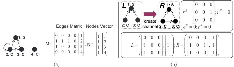
In our approach, we work with simple digraphs, which can be represented as a tuple(M,N) with M a boolean matrix for edges and N a boolean vector for nodes. The latter is necessary as in the rewriting nodes can be added and deleted. Figure1(a) shows an example of a graph representing a network of three clients and a server, where messages are depicted as self-loops. Note how we can check for well-formedness of graphs (i.e. no dangling edges) by verifying that °

°_(M∨Mt_)¯N°°

1=0, where¯is the boolean matrix product (like the regular matrix product, but with and and or instead of mutiplication and addition), andk · k1 being an operation that results in the or of all the components of the vector. We call this property compatibility.

(a) (b)

Figure 1: (a) Simple Digraph Example. (b) “Localsend” Rule.

In our framework we can assign a type to each node by a function from the set of nodes V to a set of types T , type : V →T . In Figure1(a), types are represented as an additional column in the matrices. For edges we use the types of their source and target nodes.

A production, or grammar rule, p : L→R is a partial injective morphism of simple digraphs. Using a static formulation, we can represent a rule by two boolean matrices and two vectors p=¡LE,RE; LN,RN¢, (where E stands for edges and N for nodes) to characterize the left and right hand side simple digraphs (LHS and RHS). Production p is the morphism which identifies nodes (resp., edges) on the LHS with nodes (resp., edges) on the RHS. The main actions that can be performed by a rule are deletion and addition of elements. Therefore using a dynamic formulation a rule can be represented by p=¡(LE,LN); eE_,rE_{; e}N_,rN¢_{, where e}E _{and e}N _{are the}

deletion boolean matrix and vector, while rE and rN are the addition boolean matrix and vector. The output of rule p can be calculated by R=r∨e L, where the formula applies both to nodes and edges. Superindices E and N shall be omitted if the formula applies to both cases. Moreover, we usually omit the∧(and) symbol. Figure1(b)shows a rule and its associated matrices.

and columns with zero elements and rearranges rows and columns so that the identified edges and nodes of the two graphs match.

Given a collection of productions {p1, . . . ,pn}, the notation sn =pn; pn−1;. . .; p1 defines a

sequence of productions establishing an order in their application, starting with p1 and ending with pn. Note that we may have the same production in different places of the sequence. A

concatenation is said to be coherent if actions carried out by one production do not prevent the application of those coming afterwards. Note that we assume a certain identification of nodes and edges between productions (i.e., the matrices have been completed in some way, which assumes an overlapping of the rules in the matching in the host graph). Therefore, coherence is calculated with respect to the given identification.

Theorem 1 (Sequence Coherence) The sequence sn=pn;. . .; p1is coherent if

n

_

i=1 ¡

Ri5ni+1(exry)∨Li4i1−1(eyrx)

¢

=0 (1)

where

4t1

t0(F(x,y)) = t1

_

y=t0

Ã

t1

^

x=y

(F(x,y))

!

;5t1t0(G(x,y)) = t1

_

y=t0

Ã

y

^

x=t0

(G(x,y))

!

Coherence allows the grammar designer to check dependencies between rules, and to realize possible conflicts, some of which can be solved if the initial host graph provides enough edges and nodes. This is related to the notion of minimal initial digraph, which is a graph containing the necessary nodes and edges for a sequence to be applicable.

Theorem 2 (Minimal Initial Digraph) For a coherent concatenation of productions sn=pn;. . .; p1,

its minimal initial digraph is given by the equation

Mn=5n1(rxLy) (2)

As in previous theorem, assume we have the coherent concatenation snwith minimal initial

digraph Mn, then its image is given by:

sn(Mn) = n

^

i=1

(eiMn)∨ 4n1(exry) (3)

see [VL06b] for a proof. To continue our analysis of finite sequences of productions, another useful operation is composition [VL06b]. The main difference between concatenation and com-position is the generation of intermediate states in the former. If a concatenation is coherent, then its composition can be defined. Next, we state the conditions under which a permutation of a coherent sequence remains coherent. In particular, we focus on advancement of the last production to the front and vice-versa.

Theorem 3 (Production Advance and Delay) Consider coherent sequences tn=pα; pn; pn−1;

1. φn+1(tn)is coherent if: eEα5n1 ³

rE x LEy

´

∨RE

α5n1 ³

eE x ryE

´ =0

2. δn+1(sn)is coherent if: LE_β4n1 ³

rE x eEy

´

∨rE_β4n₁

³

eE x REy

´ =0

where φn advances (i.e. moves to the right inside the concatenation) one production n−1

positions, i.e., has associated permutationφn= [1 n n−1. . .3 2]. This is a notation for

permutation cycles that means that rule 1 (the left-most one) is sent to position n, then rule in position n is moved to position n−1, and similarly until rule 3, which is moved to position 2, and this one to position 1. Operatorδn delays one production n−1 positions, i.e., hasδn =

[1 2. . .n−1 n]as associated permutation cycle (i.e. each rule is moved to the right, and rule n to position 1).

G-congruence guarantees that two coherent concatenations have the same minimal initial digraph G. The conditions to be fulfilled are known in [VL06b] as Congruence Conditions (CC). The key point is that a coherent concatenation snand a coherent permutation of it,σ(sn), which

besides have the same minimal initial digraph G (i.e., which are G-congruent) are sequential independent. Next theorem present the congruence conditions for advancement and delay of productions.

Theorem 4 (G-congruence) Given sequence sn, the congruence conditions for rule advance

(φn−1) and delay (δn−1) are given by:

CCn(φn−1,sn) = Ln∇n1−1(exry)∨rn∇1n−1(rxLy) =0 (4)

CCn(δn−1,sn) = L1∇n2(exry)∨r1∇2n(rxLy) =0 (5)

3

Algebraic Techniques for Petri Nets: The State Equation

Algebraic techniques for Petri nets are based on the representation of the net with an incidence matrix A in which columns are transitions (element Ai_j is the number of tokens that transition i removes – negative – or adds – positive – to place j). One of the problems that can be analyzed using algebraic techniques is reachability. Given an initial marking M0and a final marking Md,

a necessary condition to reach Mdfrom M0is to find a solution x for the equation Md=M0+Ax, which can be rewritten as a linear system

M=Ax (6)

Solution x – known as Parikh vector – specifies the number of times that each transition should be fired, but not the firing order. Identity (6) is known as the state equation [Mur89].

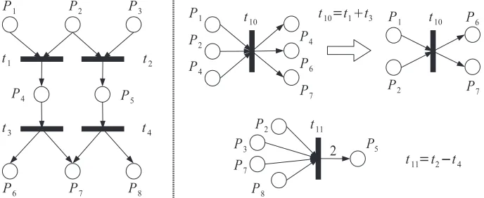
The state equation introduces a matrix, which conceptually can be thought of as associating a vector space to the dynamic behaviour of the Petri net. It is interesting to graphically interpret the operations involved in linear combinations: addition and multiplication by scalars, as depicted in Figure2. The addition of two transitions is again a transition tk=ti+tjfor which input places

appears as input and output place in tk, then it can be removed. Multiplication by −1 inverts

the transition, i.e., input places become output places and viceversa, which in some sense is equivalent to disapplying the transition.

Figure 2: Linear Combinations in the Context of Petri Nets.

One important issue is that of notation. Linear algebra uses an additive notation (addition and substraction) which is normally employed when an abelian structure is under consideration. For non-commutative structures, such as permutation groups, the multiplicative notation (com-position and inverses) is preferred. The basic operation with productions is the definition of sequences (concatenation), for which historically a multiplicative notation has been chosen, but substituting composition “◦” by the concatenation “;” operation.1

From a conceptual point of view, we are interested in relating linear combinations and se-quences of productions.2 Note that, due to commutativity, linear combinations do not have an associated notion of ordering, e.g., linear combination PV1=p1+2p2+p3coming from Parikh vector[1,2,1]can for example represent sequences p1; p2; p3; p2or p2; p2; p3; p1, which can be quite different. The fundamental concept that deals with commutativity is precisely sequential independence.

Following this reasoning, we can find the problem that makes the state equation a necessary but not a sufficient condition: some transition can temporarily owe some tokens to the net. The Parikh vector specifies a linear combination of transitions and thus, negatives are temporarily allowed (substraction).

Proposition 1 Suffiency of the state equation can only be ruined by transitions firing without

being enabled (i.e., temporarily borrowing tokens from the Petri net).

This proposition does not provide any criteria based on the topology of the Petri net, as theo-rems 16, 17, 18 and corollaries 2 and 3 in [Mur89], but contains the essential idea in their proofs: the hypothesis in previously mentioned theorems guarantee that cycles in the Petri net will not

1 _{This is the reason why [VL06b] introduces “;” to be read from right to left, contrary to the literature. Composition}

“◦” has the effect of simultaneous application, which is different to sequential application. This is important for example to differentiate sequential and parallel application.

ruin coherence.

4

Using Matrix Graph Grammars Techniques for Petri Nets

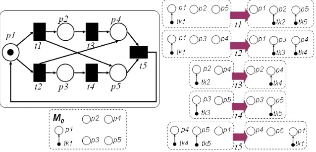
Given a Petri net, we shall consider it as the initial host graph in our matrix graph grammar. One production is associated to every transition in which places and tokens are nodes and there is an arrow joining each token to its place. In fact, we represent places for illustrative purposes only, as they are not strictly necessary, including tokens alone is enough. Figure3shows an example in which each production corresponds to a transition. The firing of a transition corresponds to the application of a rule.

Figure 3: Petri Net with Related Production set.

Thus, Petri nets can be considered a proper subset of graph grammars with two important properties:

1. There are no dangling edges when applying productions (firing transitions).

2. Every production can be applied only in one part of the host graph.

Properties (1) and (2) somehow allow us to safely “ignore” matchings as introduced in [VL06a]. In addition, we consider Petri nets with no self-loops (i.e., so called pure Petri nets), that is, one production either adds or deletes nodes of a concrete type, but there is never a simultaneous addition and deletion of nodes of the same type. This agrees with the expected behaviour of MGG productions with respect to nodes (which is the behaviour of edges as well, see [VL06b]) and will be kept throughout the present work, mainly because rules in SPO-like grammars are adapted depending on whether a given production deletes nodes or not (refer to section6). Hence, it is necessary that elements in matrices are not relative integers, i.e., a number four must mean that production x adds four nodes of type t and not that x adds four nodes more than it deletes of type t. If we had one such production p, a possible way to proceed is to split p into two, one owning the addition actions, pr, and the other the deletion ones, pe. Sequentially, p should be

Minimal Marking. The concept of minimal initial digraph can be used to find the minimum marking able to fire a given transition sequence. For example, Figure4 shows the calculation of the minimal marking able to fire transition sequence t5;t3;t1(from right to left). Notice that (r1L1)∨(r1L2)(r2L2)∨ · · · ∨(r1Ln)· · ·(rnLn)is the expanded form of equation2.

Figure 4: Minimal Marking Firing Sequence t5;t3;t1.

Reachability. The reachability problem can also be expressed using MGG concepts, as the following definition shows.

Definition 1 (Reachability) Given a grammar G= (M0,{p1, . . . ,pn}), a state Md is called

reachable starting in state M0, if there exists a coherent concatenation made up of productions pi∈Gwith minimal initial digraph contained in M0and image in Md.

5

Reachability: DPO-Like Matrix Graph Grammars

In this and next sections we shall be concerned with the generalization of the state equation to wider types of grammars. By a DPO-like matrix graph grammar we understand a grammar as introduced in [VL06b], but in which rule applications do not generate dangling edges. That is, in any reachable graph from the initial one, no rule application can generate a dangling edge (i.e. the dangling condition in classical Double Pushout graph grammars [EEPT06] can be safely ignored as it can never happen). Property 2in section4 of Petri nets is relaxed because now a single production may eventually be applied in several different places of the host graph. However, following the discussion in previous section, we restrict to DPO rules in which nodes (or edges) of the same type are not rewritten (deleted and created) in the same rule.

In order to perform an a priori analysis it is mandatory to get rid of matches. To this end, either an approach as proposed in [VL06a,VL06b] is followed (as we did in this paper in section4), or types of nodes are taken into account instead of nodes themselves. Here, we take this second alternative, therefore productions, initial state and final state are transformed such that types of elements are considered, obtaining matrices with elements inZ.

Though it shall be avoided whenever possible, four index may be used simultaneously, E₀Ai_j. Top left index indicates whether we are working with nodes (N) or edges (E). Bottom left index specifies the position inside a sequence, if any. Top right and bottom right are contravariant and covariant indices, respectively.

Definition 2 LetG= (0M,{p1, . . . ,pn}) be a DPO-like graph grammar and m the number of

different types of nodes inG. The incidence matrix for nodesNA=¡Ai_k¢where i∈ {1, . . . ,n} and k∈ {1, . . . ,m}is defined by the identity

Ai_k= ½

+r if production k adds r nodes of type i

−r if production k deletes r nodes of type i (7)

It is straightforward to deduce for nodes an equation similar to (6):

N

dMi=N0Mi+

n

∑

k=1

N_Ai

kxk (8)

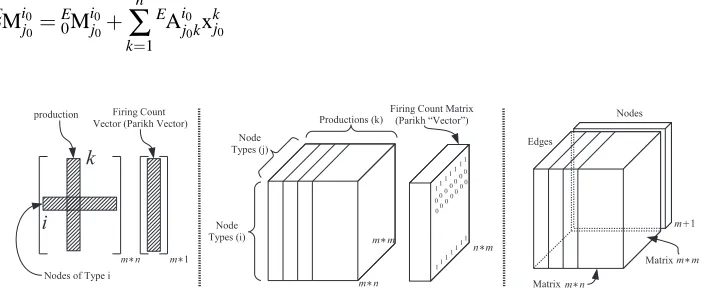
The case for edges is similar, with the peculiarity that edges are represented by matrices instead of vectors and thus the incidence matrix becomes the incidence tensorEAi_jk. Again, only types of edges, and not edges themselves, are taken into account. Two edges e1 and e2 are of the same type if their starting and final nodes are of the same type. Initial nodes of edges will be assumed to have a contravariant behaviour (index on top, i) while terminal nodes (first index, j) and productions (second index, k) will behave covariantly (index on bottom). See diagram in the center of Figure6.

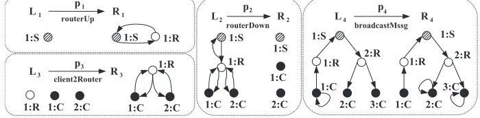
Example.¤Some rules for a simple client-server system adapted from [VL06a] are defined in

Figure5. There are three types of nodes: clients (C), servers (S) and routers (R). Messages (self-loops in clients) can only be broadcasted. In the MGG approach, this transformation system will behave SPO or DPO-like depending on the initial state. Note that production p4adds and deletes edges of the same type(C,C). By now, the rule will not be split into its addition and deletion components as suggested in4. See section6.1for an example.

Figure 5: Rules for a Client-Server Broadcast-Limited System.

Incidence tensor (edges) for these rules can be represented componentwise, each component being the matrix associated to the corresponding production.

E_Ai j1=



 0₀ 0₀ 0₁ C_R

0 1 0 S



_;E_Ai j2=



 ₋0₂ −2_{0 −}0₁

0 −1 0



_;E_Ai j3=



 0₂ 2₀ 0₀ 0 0 0



_;E_Ai j4=



 1₀ 0₀ 0₀ 0 0 0



For space limitations, only inEAi_j1we have specified which type each row belongs to. Columns follow the same ordering.¥

Lemma 1 With notation as above, a necessary condition for state dM to be reachable from

state0M is

dM−0M=EM=EMij= n

∑

k=1

E_Ai jkxkj=

n

∑

k=1,p=k

¡_E

A⊗x¢ip_jk (9)

where i,j∈ {1, . . . ,m}.

Proof

¤Consider the construction depicted in the center of figure6in which tensor Ai_jk is represented as a cube. A product for this object is informally defined in the following way: every vector in the cube perpendicular to matrix x acts on the corresponding row of the matrix in the usual way, i.e., for every fixed i=i0and j= j0in (9):

E

dMi0j0 =E0Mi0j0+ n

∑

k=1

E_Ai0 j0kx

k

j0 (10)

Figure 6: Matrix Representation for Nodes, Tensor for Edges and Their Coupling.

Every column in matrix x is a Parikh vector as defined for Petri nets. Its elements specify the amount of times that every production must be applied, so all rows must be equal and hence, equation (10) needs to be enlarged with some additional identities

 



Mi_j =

n

∑

k=1

E_Ai jkxkj

xk_p = xk_q

(11)

with p,q∈ {1, . . . ,m}. This uniqueness together with previous equations provide the intuition to raise (9).

Informally, we are enlarging the space of possible solutions and then projecting according to some restrictions. To see that it is a necessary condition, suppose that there exists a sequence sn

such that sn(0M) =dM and that equation (10) does not provide any solution. Without loss of

from the first node), which produces an equation completely analogous to the state equation for Petri nets, deriving a contradiction.¥

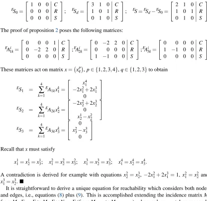
Example (Cont’d).¤Let’s test whether it is possible to move from state S0 to state Sd (see

Figure7) with the productions defined in previous example.

Figure 7: Initial and Final States for Productions in Fig.5.

Matrices for the states (edges only) and their difference are:

E_S

0= 

 1₀ 0₀ 0₀ C_R

0 0 0 S



_; E_S d=



 3₁ 1₀ 0₁ C_R

0 1 0 S



_; E_S=E_S

d−ES0= 

 2₁ 1₀ 0₁ C_R

0 1 0 S





The proof of proposition2poses the following matrices:

E_Ai

1k= 

 0_{0 −}0₂ 0₂ 1₀ C_R

0 0 0 0 S



_;E_Ai

2k= 

 0₀ −2₀ 2₀ 0₀ C_R 1 −1 0 0 S



_;E_Ai

3k= 

 0_{1 −}0₁ 0₀ 0₀ C_R

0 0 0 0 S





These matrices act on matrix x=¡xqp

¢

, p∈ {1,2,3,4}, q∈ {1,2,3}to obtain

E_S 1 = 4

∑

1kxk1= 

 x

4 1

−2x2₁+2x3₁ 0   E_S 2 = 4

∑

2kxk2= 

 −2x 2 2+2x32

0 x1₂−x2₂

  E_S 3 = 4

∑

3kxk3= 

 _x2 0 3−x33

0 



Recall that x must satisfy

x1₁=x1₂=x1₃; x2₁=x2₂=x2₃; x3₁=x3₂=x3₃; x4₁=x4₂=x4₃.

A contradiction is derived for example with equations x2₂ =x3₂, −2x2₁+2x₁3=1, x2₁ =x2₂ and x3₁=x3₂.¥

Definition 3 (Incidence Tensor) Given a grammarG= (0M,{p1, . . . ,pn}), the incidence tensor

Ai_jkwith i∈ {1, . . . ,m}and j∈ {1, . . . ,m+1}is defined by (9) if 1≤j≤m and by (8) if j=m+1.

Note that top left index in our notation works as follows:NA refers to nodes,EA to edges and A to their coupling. An immediate extension of lemmata1is:

Proposition 2 (State Equation for DPO-like Matrix Grammars) With notation as above, a

nec-essary condition for statedM to be reachable (from state0M) is

M_ij=

n

∑

k=1

Ai_jkxk (12)

Notice that equation (12) is a generalization of the state equation (6) for Petri nets.

6

Reachability: SPO-like matrix graph grammars

Our intention now is to relax the second property of Petri nets and allow production application even though some dangling edge might appear (see [VL06a,VL06b]). The plan is carried out in two stages which correspond to the subsections that follow, according to the classification of ε-productions in [VL06a].

In our approach, if applying a production p0 causes dangling edges, the production can be applied but a new production (a so-calledε-production) is created and applied first. In this way, we obtain a sequence p0; pε0, with the restriction that pε0 is applied at a match that includes all nodes deleted by p0that produce dangling edges. Production pε0deletes the dangling edges produced by p0, and then p0can be applied, without producing dangling edges (see [VL06a] for details).

Inside a sequence, a production p0that deletes an edge or node can have an external or internal behaviour, depending on the identification carried out by the match. Following [VL06a], if the deleted element was added or used by a previous production, we shall label the production as internal (according to the sequence). On the other hand, if the deleted element is provided by the host graph and it is not used until p0’s turn, then p0is an external production. In some sense, their properties are complementary: while externalε-productions can be advanced and composed to eventually get a single initial production which adapts the host graph to the sequence, internal ε-productions are more static3in nature. On the other hand, internal ε-productions depend on productions themselves and are somewhat independent of the host graph, opposite to external ε-productions. Note however that internal nodes can be unrelated if, for example, matchings identify them in different parts of the host graph, thus becoming external.

6.1 External

ε

The main property of externalε-productions, with respect to internalε-productions, is that they act only on edges that appear in the initial state, so their application can be advanced to the beginning of the sequence. In this situation, the first thing to know for a given matrix graph

grammarG= (0M,{p1, . . . ,pn})with at most externalε-productions when applied to0M, is the maximum number of edges that can be erased from its initial state. The potential dangling edges (those with any incident node to be erased) are given by:

e=

n

_

k=1 ³

N ke⊗Nke

´

(13)

Proposition 3 Given a grammar G= (0M,{p1, . . . ,pn}) with externalε-productions only, a

necessary condition for statedM to be reachable (from state0M) is

Mi_j=

n

∑

k=1 ³

Ai_jkxk

´

+bi_j (14)

with the restriction0Me≤bi_j≤0.

Note that equation (12) in proposition 2 is recovered from (14) if there are no external ε -productions.

According to [VL06a], allε-productions can be advanced to the beginning of the sequence and be composed to obtain a single production, adapting the initial digraph before applying the sequence, which in some sense interprets matrix b as the production number n+1 in the sequence (i.e. the first to be applied). Because it is not possible to know in advance the order of application of productions, all we can do is to provide bounds for the number of edges to be erased.

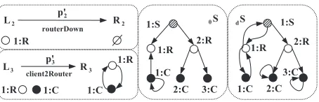
Example. Consider the initial and final states shown in Figure 8. Productions of previous

examples are used, but two of them are modified (p2and p3).

Figure 8: Initial and Final States with Amendments to Some Productions of Fig.5.

In this case there are sequences that transform state0S indS, for example, s4=p4; p1; p0₃; p0₂. Note that the problem is in edge(1 : S,1 : R)of the intial state: router 1 is able to receive packets from server 1, but not to send them.

Next, matrices for the states and their difference are calculated. The first three columns corre-spond to edges (first to clients, second to routers and third to servers), fourth to nodes and fifth specifies types.

0S= 

 1₂ 1₀ 0₀ 3₂ C_R

0 2 0 1 S



_{; dS=} 

 2₃ 1₀ 0₁ 3₂ C_R

0 2 0 1 S



_{; S=dS−0S=} 

 1₁ 0₀ 0₁ 0₀ C_R

0 0 0 0 S



The incidence tensors for every production (recall that p2 and p3 are as in Figure 8) have the form

Ai_j1=



 0₀ 0₀ 0₁ 0₁

0 1 0 0



_{; A}i j2=



 _{0 −}0₁ 0



_{; A}i j3=



 0₁ 1₀ 0₀ 0₀

0 0 0 0



_{; A}i j4=



 1₀ 0₀ 0₀ 0₀

0 0 0 0





Though it does not seem to be strictly necessary here, more information is kept and calculations are more flexible if production p4is split in the part that deletes messages and the part that adds them, p4=p4r; p4e. See comments about this in section4

Ai_j4e=



 −₀1 0₀ 0₀ 0₀ C_R

0 0 0 0 S



_{; A}i j4r=



 2₀ 0₀ 0₀ 0₀ C_R

0 0 0 0 S





As in the example of section5, the following matrices are more appropriate for calculations:

A_1ki =



 0₀ 0₀ 0₁ −₀1 2₀

0 0 0 0 0



_{; A}i

2k= 

 0₀ 0₀ 1₀ 0₀ 0₀

1 0 0 0 0



_{; A}i

3k= 

 0₁ 0₀ 0₀ 0₀ 0₀

0 0 0 0 0



_;

A_4ki =



 0_{1 −}0₁ 0₀ 0₀ 0₀

0 0 0 0 0





If (12) is directly applied, we obtain x1=0 and x1=1 (third row of A_2ki and second of A_3ki ) deriving a contradiction. The variations permitted for the initial state are given by the matrix

0Me= 

 0 α 1 2 0 0 α2

1 0 0 0 0 α3

2 0 0 

 ₍₁₅₎

Withα₂1∈ {0,−1},α2

1,α23∈ {0,−1,−2}. Setting b21=−1 and b32=−1 (one edge(S,R)and one edge(C,R)removed) the system to be solved is



 1₁ 1₀ 0₁ 0₀

0 1 0 0



₌ 

 −x

4_+2x4 _x3 _{0 0} x3 0 x1 x1−x2

0 x1 0 0





with solution x1=x2 =x3 =x4=1, s4 being one of its associated sequences. Note that the restriction in proposition3is fulfilled, see (15).

In previous example, as we knew a sequence (s4) answer to the reachability problem, we have fixed matrix b directly to show how proposition3works. Although this will not be normally the case, the way to proceed is very similar: relax matrix M by substracting b, find a set of solutions

6.2 Internal

ε

Internal ε-productions delete edges appended or used by productions preceding it in the se-quence. In this subsection we first limit to sequences which may have only internalε-productions and, by the end of the section, we shall put together proposition3from subsection6.1with results derived here to state theorem5for SPO-like matrix graph grammars.

The way to proceed is completely analogous to that of external ε-productions. The idea is to allow some variation in the amount of edges erased by every production, but this variation is constrained depending on the behaviour (definition) of the rest of the rules. Unfortunately, not so much information is gathered in this case and what we are basically doing is ignoring this part of the state equation.

Define hi_jk= h

Ai_jk(e⊗Ik)

i

+=max(A(e⊗I),0), whereIk= [1, . . . ,1](1,k). 4

Proposition 4 Given a grammar G= (0M,{p1, . . . ,pn}) with internalε-productions only, a

necessary condition for statedM to be reachable (from state0M) is

Mi_j=

n

∑

k=1 ¡

Ai_jk+V¢xk (16)

with the restriction hi_jk≤V_jki ≤0.

In some sense, external productions are the limiting case of internal productions and can be seen almost as a particular case: asε-productions do not interfere with previous productions they have to act exclusively on the host graph. The full generalization of the state equation for matrix graph grammars is:

Theorem 5 (State Equation) With previous notation, a necessary condition for statedM to be

reachable (from state0M) is

Mi_j=

n

∑

k=1 ¡

Ai_jk+V¢xk+bi_j (17)

bi_jmust satisfy restrictions specified in proposition3and V those in proposition4.

Strengthening hypothesis, formula (5) becomes those already studied for SPO with internal ε-productions (b=0), with externalε-productions (V=0), DPO-like (from multilinear to linear transformations) or Petri nets, fully recovering the original form of the state equation.

7

Related Work

Concerning our MGG approach to graph rewriting, in [Val98] an implementation of the DPO cat-egorical approach to graph transformation was implemented using Mathematica. In that work, (simple) digraphs were represented with their boolean adjacency matrices. This is the only sim-ilarity with our work, as our goal is to develop a theory for (simple) graph rewriting based on

boolean matrix algebra. Other somehow related approach is the relational approaches of [MK95] and [Kah02]. However, they rely on using category theory for expressing the rewriting.

The recent work [VVE+06] shows a means to encode a graph transformation system into a Petri net. Then algebraic approaches based on the state equation can be used for analysis. The approach is similar to ours, as they perform the same abstraction (taking node and edge types). However, on the one hand, they consider negative application conditions in rules. On the other hand, we consider both DPO and SPO-like grammars, and we extend the state equation using tensors, instead of first encoding the transformation system as a Petri net.

8

Conclusions and Future Work.

The starting point of the present paper is the study of Petri nets as a particular case of MGGs. Next, reachability and the state equation have been reformulated and extended with the language of this new approach, trying to provide tools for grammars as general as possible. The objective is almost fulfilled, bearing in mind that the more general the grammar, the less information the state equation provides. For example, equation (12) is more accurate as long as the rate of the amount of types of nodes with respect to the amount of nodes approaches one. Hence, in general, it will be of little practical use if there are many nodes but few types.

Nevertheless, we are in a much better position than we were before. Although the use of vector spaces (as in Petri nets) and multilinear algebra is almost straightforward, many other algebraic structures are available to improve the results herein presented. For example, Lie algebras seem a good candidate if we think of the Lie bracket as a measure of commutativity (recall subsection 3in which we saw that this is one of the main problems of using linear combinations).

Other concepts and techniques from Petri nets such as invariants, boundedness, liveness, re-versibility, persistence, etc., can also be extended to more general grammars. Besides, it is possible as well to get a better insight and understanding of matters by applying matrix graph grammars techniques (as those in [VL06a,VL06b] and the present paper) to Petri nets. We are also extending our matrix graph grammars approach to work with multi-graphs. A first line of attack is to model edges as special nodes (with exactly one incoming and outgoing edge).

Acknowledgements: This work has been sponsored by the Spanish Ministry of Science and

Education, project MOSAIC (TSI2005-08225-C07-06). The authors would like to thank the referees, the workshop participants and Alejandro P´erez Velasco for their useful suggestions.

References

[EEPT06] H. Ehrig, K. Ehrig, U. Prange, G. Taentzer. Fundamentals of Algebraic Graph Transformation. Monographs in Theoretical Computer Science, an EATCS series. Springer, Berlin, Heidelberg, New York, 2006.

[MK95] Y. Mizoguchi, Y. Kuwahara. Relational Graph Rewritings. Theoretical Computer Science 141:311–328, 1995.

[Mur89] T. Murata. Petri nets: Properties, analysis and applications. Proceedings of the IEEE 77(4):541–580, April 1989.

[Sok51] I. S. Sokolnikoff. Tensor Analysis, Theory and Applications. Applied Mathematics series. John Wiley and Sons, New York, 1951.

[Val98] G. Valiente. Grammatica: An Implementation of Algebraic Graph Transformation on Mathematica. In Proc. Sixth Workshop on Theory and Application of Graph Transformations. Pp. 261–267. 1998.

[VL06a] P. P. P. Velasco, J. de Lara. Matrix Approach To Graph Transformation: Match-ing and Sequences. In Proc. ICGT’06. Lecture Notes in Computer Science 4178, pp. 122–137. Springer-Verlag, 2006.

[VL06b] P. P. P. Velasco, J. de Lara. Towards a New Algebraic Approach to Graph Transfor-mation: Long Version. Technical report, Universidad Aut´onoma de Madrid, 2006.