Vol 9, No 1 (2018)

(1)

Available online throug

ISSN 2229 – 5046

International Journal of Mathematical Archive- 9(1), Jan. – 2018 151

MELTING HEAT TRANSFER OF UNSTEADY MHD BOUNDARY LAYER

FLOW OF EYRING-POWELL NANOFLUID PAST AN INCLINED STRETCHING SHEET

VIJAYA BHASKAR REDDY.N*

1

_{, KISHAN NAIKOTI}

2

1

_{Government Degree College (Autonomous),}

Siddipet Dist., Telangana state, India, 502103.

2

_{Department of Mathematics, University College of Science,}

Osmania University, Hyderabad, Telangana state, India, 500007.

(Received On: 24-11-17; Revised & Accepted On: 20-12-17)

ABSTRACT

T

his paper deals with the viscous incompressible magnetohydrodynamic boundary layer unsteady flow of an Eyring-Powell nanofluid over an inclined melting stretching sheet in the presence of radiation and non-uniform heat source/sink effects has been investigated numerically. The resulting nonlinear governing partial differential equations with associated boundary conditions of the problem has formulated and transformed into a non-similar form. The resultant equations are then solved numerically using Runge-Kutta fourth order method along with shooting technique. The physical significance of different parameters on the velocity, temperature and nanoparticle volume fraction profiles are discussed through graphical illustrations. The impact of physical parameters on local skin friction coefficient, the rate of heat transfer and rate of mass transfer are shown in the tabulated form.

Keywords: Eyring-Powell fluid, Melting heat transfer, MHD, Inclined Stretching sheet, Brownian motion, Radiation,

Unsteady.

1. INTRODUCTION

The study of heat transfer over a stretching surface has significant importance due to numerous applications in industrial and technological processes such as cooling of metallic sheets, glass fibres, extrusion of the polymer sheet, and boundary layer along liquid films in concentration processes, paper production and metal spinning. The rate of heat transfer at the stretching surface affects deeply the quality of the final products which must fulfil the desired specifications. Crane [1] was the first investigated an exact analytical solution for the steady two-dimensional flows due to a stretching surface in a quiescent fluid. After this pioneering work, the ﬂow ﬁeld over a stretching surface has drawn considerable attention and a good amount of research has been investigated on this problem [2–5].

The mathematical formulation for flows of non -Newtonian fluids, in general, is more complex. The most frequently used models of non-Newtonian models are the second grade, Maxwell, Oldroyd-B and power law. A broad description of the behaviour in both steady and unsteady flow situations, together with mathematical models can be found in Refs . [6–10]. The Powell-Eyring model has certain advantages over the other non-Newtonian fluid models. Firstly, it is deduced from the kinetic theory of liquids rather than the empirical relation. Secondly, it correctly reduces to Newtonian behaviour for low and high shear rates. The study of Powell-Eyring fluid has attracted the researchers of fluid dynamics due to its numerous applications in science and technology. Patel and Timol[11] numerically examined the flow of Powell-Eyring model through asymptotic boundary conditions. Hayat et al. [12] studied the steady flow of Powell-Eyring fluid over a moving surface with convective boundary conditions. Flow and heat transfer of Powell-Eyring fluid over shrinking surface in a parallel free stream is presented by Rosca and Pop [13]. Jalil et al. [14] studied the flow and heat transfer of Powell-Eyring fluid over a moving surface in a parallel free stream. The problem of slider bearing lubricated with Eyring Powell model is presented numerically using Homotopy perturbation analysis by Islam et al. [15]. Regarding the study of Powell-Eyring on fluid flow and heat transfer, some former attentions have been made in the studies [16, 17]. The flow and heat transfer of Powell-Eyring fluid over a continuously moving surface in the presence of a free stream velocity is investigated by Hayat et al. [18].

Corresponding Author: Vijaya Bhaskar Reddy.N*

1

_,

(2)

Due to the small size and very large specific surface areas of nanoparticles, nanofluids have superior properties like high thermal conductivity, minimal clogging in flow passages, long-term stability, and homogeneity. Thus, nanofluids have a wide range of potential applications in electronic cooling, pharmacological administration mechanisms, peristaltic pumps for diabetic treatments, solar collectors and nuclear applications. Based on these real-world applications, Choi[19] has introduced the concept of nanofluid in order to develop advanced heat transfer fluids with substantially higher conductivities. Later on, the boundary layer flow of nanofluid past a stretching surface under the effect of Brownian motion and thermophoresis was investigated by Khan and Pop [20]. Kuznetsov and Nield [21] investigated the natural convective boundary-layer flow of nanofluid past a vertical plate by incorporating Brownian motion and thermophoresis effects. Gorla et al. [22] have reported the numerical solutions for a steady boundary layer flow of nanofluid on a stretching circular cylinder in a stagnant free stream. Rajesh Vemula et al. [23] analyzed unsteady MHD Free convection flow of nanofluid past an accelerated vertical plate with variable temperature and thermal radiation. The unsteady two-dimensional flow of a non-Newtonian fluid over a stretching surface having a prescribed surface temperature is investigated by Mukhopadhyay et al. [24].

Melting and solidification play a vital role in the advanced technology process. Researchers are interested to explore melting heat transfer due to a wide range of application of melting phenomenon of solid-liquid phase change materials in the welding process, crystal growth, thermal protection, heat transportation melting of permafrost, preparation of semiconductors material and the casting of a manufacturing process. Initially, Robert [25] described the melting phenomenon of ice slab placed in a hot air stream. Boundary layer stagnation point flow of Maxwell fluid towards a stretching sheet with melting phenomenon is analyzed by Hayat et al. [26]. Das [27] discussed the melting phenomenon in the magnetohydrodynamic flow over a moving surface with thermal radiation. Melting heat transfer in steady laminar flow over a stationary flat plate has been studied by Epstein and Cho [28] Then after, Kazmierczak et al. [29] studied the steady convection flow over a flat plate embedded in a porous medium with melting heat transfer effect. Gorla et al. [30] have studied the melting heat transfer in mixed convection flow over a vertical plate. Recently, an analysis has been carried out by Bachok et al. [31] to analyze a steady two-dimensional stagnation point flow and heat transfer over a melting stretching sheet.

Over the last few years, a considerable amount of experimental and theoretical work has been carried out to determine the role of natural convection in the kinetics of heat transfer accompanied with melting or solidification effect. Processes involving melting heat transfer in non-Newtonian fluids have promising applications in thermal engineering, such as oil extraction, magma, solidification, melting of permafrost, geothermal energy recovery, silicon wafer process, thermal insulation, etc. Chamkha et al. [32] analysed the effect of the transverse magnetic field on hydromagnetic, forced convection flow with heat and mass transfer of a nanofluid over a horizontal stretching plate under the influence of melting and heat generation or absorption. Gorla et al. [33] presented a boundary layer analysis for a warm and laminar flow of nanofluid over a melting surface moving parallel to a uniform free stream.

Recently, P. Mohan Krishna, N. Sandeep et al. [38] investigated the unsteady flow of Powell Eyring fluid past an inclined stretching sheet in the presence of radiation, non-uniform heat source/sink and chemical reaction. The main emphasis of the current paper deals with the two-dimensional unsteady flow of a Powell-Eyring nanofluid past a melting stretching inclined in the presence of radiation and non-uniform heat source/sink with chemical reaction. To achieve this study the suitable transformation is used to transform the partial differential equations to a system of ordinary differential equations together with boundary Conditions the resulting system of ordinary differential equations are solved using the well-known Runge-Kutta technique along with shooting method.

2. MATHEMATICAL FORMULATION

Consider an incompressible, two-dimensional unsteady MHD boundary layer flow of an electrically conducting Powell-Eyring fluid past an inclined stretching sheet in the presence of nanoparticles. A magnetic field of strength B0(t)

is applied normal to the sheet along the y-direction. It is also assumed that, 𝑇_𝑚 and 𝐶_𝑚 represents the surface temperature and concentration of nanoparticles at the sheet respectively, while 𝑇_∞ and 𝐶_∞ respectively denote the ambient fluid temperature and concentration. It is assumed that the Reynolds number is small so that an induced magnetic field is neglected. The applied transverse magnetic field is assumed to be variable kind and is considered in the special form as 𝐵(𝑡) = 𝐵0

(1−𝑎𝑡)1/2. The sheet makes an angle

α

with the vertical direction and the x-axis is taken

along the sheet and y-axis is normal to it. In addition, we considered the effects of thermal radiation, chemical reaction and non-uniform heat source/sink.

(3)

µ

stands for dynamic viscosity 𝛽_and𝑐₁ for material fluid constants. Considering

𝑠𝑖𝑛ℎ−1_�1 𝑐1

𝜕𝑢𝑖

𝜕𝑥𝑗�=�

1 𝑐1

𝜕𝑢𝑖

𝜕𝑥𝑗−

1 6�

1 𝑐1

𝜕𝑢𝑖

𝜕𝑥𝑗�

3 ,�_𝑐1

1

𝜕𝑢𝑖

𝜕𝑥𝑗� ≪1

The boundary layer expressions for two-dimensional magnetohydrodynamic flow of Powell-Eyring nanofluid are as

follows(see Rosca and Pop[13], Jalil et al. [14]): 𝜕𝑢

𝜕𝑥+ 𝜕𝑣

𝜕𝑦= 0 (1) 𝜕𝑢

𝜕𝑡+𝑢 𝜕𝑢 𝜕𝑥+𝑣

𝜕𝑢 𝜕𝑦=𝜈

𝜕2_𝑢

𝜕𝑦2+

1 𝜌𝛽𝐶1

𝜕2_𝑢

𝜕𝑦2−

1 𝜌𝛽𝐶13 �

𝜕𝑢 𝜕𝑦�

2 𝜕2_𝑢

𝜕𝑦2

-𝜎

𝜌𝐵2(𝑡)𝑢+ [𝑔𝐵𝑇(𝑇 − 𝑇∞) +𝑔𝐵𝑐(𝐶 − 𝐶∞)]𝑐𝑜𝑠𝛼 (2) 𝜕𝑇

𝜕𝑡+𝑢 𝜕𝑇 𝜕𝑥+𝑣

𝜕𝑇 𝜕𝑦=

𝑘 𝜌𝑐𝑝

𝜕2𝑇 𝜕𝑦2−

1 𝜌𝑐𝑝

𝜕𝑞𝑟

𝜕𝑦 +𝜏 �𝐷𝐵 𝜕𝐶 𝜕𝑦

𝜕𝑇 𝜕𝑦+

𝐷𝑇

𝑇∞�

𝜕𝑇 𝜕𝑦�

2

�+𝑞′′′ (3) 𝜕𝐶

𝜕𝑡+𝑢 𝜕𝐶 𝜕𝑥+𝑣

𝜕𝐶 𝜕𝑦=�𝐷𝐵

𝜕2𝐶 𝜕𝑦2+𝐷_𝑇_∞𝑇𝜕

2_𝑇

𝜕𝑦2�-𝑘𝑙(𝐶 − 𝐶∞) (4) Where t is the time, u and v are the velocity components along x- and y-axis, 𝜀and 𝛿 are Powell-Eyring fluid

parameters, 𝜈 �= 𝜇

𝜌𝑓�stands for kinematic viscosity, k is the thermal conductivity of the fluid, 𝜌𝑓 is the fluid density, T

is the fluid temperature, C is the fluid nanoparticle volume fraction, 𝜏 �=(𝜌𝑐)𝑝

(𝜌𝑐)_𝑓� is the ratio between the effective heat capacity of the nanoparticle material and heat capacity of the fluid(see Oyelakin et al. [37]), 𝐷_𝑇 for thermophoresis diffusion constant, 𝐷𝐵 _{for Brownian diffusivity constant,}𝑐_𝑝 is the specific heat, g is the acceleration due to gravity, 𝛽𝑇and 𝛽𝐶 is the volumetric coefficient of thermal and mass exponential, 𝐾𝑙 is the chemical reaction parameter,

𝑞𝑟=−16𝜎

∗_𝑇_∞3

3𝑘∗ 𝜕𝑇_𝜕𝑦 is the linearized radiative heat flux, 𝛼is the inclined angle, is 𝑘∗ the mean absorption coefficient, 𝜎∗is

the Stefan-Boltzmann constant, is the non-uniform heat source/sink per unit volume. The non-uniform heat source/sink, 𝑞′′′is modelled by the following expression

𝑞′′′₌𝑘𝑈𝑚(𝑥,𝑡)

𝑥𝜈 [𝐴∗(𝑇𝑚− 𝑇∞)𝑓′+𝐵∗(𝑇 − 𝑇∞)]

In which 𝐴∗and 𝐵∗ are the coefficients of space and temperature dependent heat source/sink, respectively. Here two cases arise, for internal heat generation 𝐴∗> 0 and 𝐵∗> 0_{and for internal heat absorption, we have}𝐴∗< 0 and 𝐵∗_{< 0}_.

The surface velocity is denoted by 𝑢𝑚(𝑥,𝑡) = 𝑏𝑥 (1−𝑎𝑡) where as the surface temperature is 𝑇_𝑚(𝑥,𝑡) =𝑇_∞+𝑇_𝑟𝑒𝑓𝑏𝑥2

𝜈 (1− 𝑎𝑡)−3/2 and surface concentration is

𝐶𝑚(𝑥,𝑡) =𝐶∞+𝐶𝑟𝑒𝑓𝑏𝑥

2

𝜈 (1− 𝑎𝑡)−3/2 and time dependent magnetic field B(t) is 𝐵(𝑡) = 𝐵0

(1−𝑎𝑡)1/2.

Here b is the initial stretching rate, a is the positive constant which measures the unsteadiness. Also 𝑇𝑟𝑒𝑓,𝐶_𝑟𝑒𝑓 are constant reference temperature and nanoparticle volume fraction respectively.

The associated boundary conditions are

𝑢=𝑢𝑚(𝑥,𝑡),𝑇=𝑇𝑚(𝑥,𝑡), 𝐶=𝐶𝑚(𝑥,𝑡) 𝑎𝑡𝑦= 0 (5)

𝑢 →0,𝑇 → 𝑇∞,𝐶 → 𝐶∞ 𝑎𝑠𝑦 → ∞ (6) And𝑘 �𝜕𝑇

𝜕𝑦�_𝑦=0=𝜌[𝜆+𝐶𝑠(𝑇𝑚− 𝑇0)]𝑣(𝑥, 0) (7)

and 𝑢_𝑚(𝑥,𝑡) = 𝑏𝑥

(1−𝑎𝑡) here b is the initial stretching rate, a is the positive constant which measures the unsteadiness. We have 𝑏

(1−𝑎𝑡) in the initial stretching rate that increases with time, 𝑇𝑚,𝐶𝑚are the surface temperature and surface concentration and 𝑇∞,𝐶_∞are the ambient fluid temperature and concentration respectively. Further, k is the thermal conductivity, 𝜆is the latent heat of the fluid and 𝑐_𝑠is the heat capacity of the solid surface. Equation (7) states that the heat conducted to the melting surface is equal to the heat of melting plus the sensible heat required to raise the solid surface temperature 𝑇₀to its melting temperature 𝑇_𝑚.

Introducing the following similarity transformations

𝑢=₍_1−𝑎𝑡𝑏𝑥 ₎𝑓′₍_𝜂_),_𝑣₌_−� 𝜈𝑏

(1−𝑎𝑡)𝑓(𝜂

𝜂=𝑦�_𝜈₍_1−𝑎𝑡𝑏 ₎,𝜃(𝜂) = 𝑇−𝑇∞

𝑇𝑚−𝑇∞,𝜙(𝜂) =

𝐶−𝐶∞

𝐶𝑚−𝐶∞⎭

⎬ ⎫

(4)

By using above similarity transformations the equations (1) -(4) reduces to

(1 +𝜖)𝑓′′′₊_𝑓𝑓′′_{− 𝑓}′2_{− 𝜀𝛿𝑓}′′2_𝑓′′′_{− 𝐴 �𝑓}′₊1

2𝜂𝑓′′� − 𝑀𝑓′+ [𝐺𝑟𝜃+𝐺𝑐𝜙]𝑐𝑜𝑠𝛼= 0 (9)

�1 +4₃𝑅𝑑� 𝜃′′₊_{𝑃𝑟 �𝑓𝜃}′₋₂_𝑓′_{𝜃 −}1

2𝐴(3𝜃+𝜂𝜃′) +𝑁𝑏𝜃′𝜙′+𝑁𝑡𝜃′2�+𝐴∗𝑓′+𝐵∗𝜃 = 0 (10)

𝜙′′_{− 𝐿𝑒 �}₂_𝜙𝑓′_{− 𝑓𝜙}′₊1

2𝐴(3𝜙+𝜂𝜙′) +𝐾𝑟𝜙�+ 𝑁𝑡

𝑁𝑏𝜃′′= 0 (11) and the boundary conditions(5)-(7) are reduced to

𝑃𝑟𝑓[0] +𝑀𝑒𝜃′_{[0] = 0,}_𝑓′_{[0] = 1,}_𝜃_{[0] = 1,}

𝜙[0] = 1,𝑓′_[_∞_]_→_0,_𝜃_[_∞_]_→_0,_𝜙_[_∞_]_→₀� (12)

Here 𝜀 and 𝛿 stand for fluid parameters, Pr for Prandtl number, Me is the dimensionless melting parameter, M for magnetic parameter, Gr for thermal Grashof number, Gc for solutal Grashof number, Nt for thermophoresis parameter, Nb for Brownian motion parameter and Le for Lewis number, Rd for radiation parameter, A for unsteadiness parameter, Kr for chemical reaction parameter.

These parameters are defined by 𝑃𝑟=𝜇𝑐𝑝

𝑘 ,𝜖= 1 𝜇𝛽𝑐1,𝛿=

𝑢𝑚3

2𝜈𝑥𝒄_𝟏𝟐,𝑀𝑒=

𝑐𝑝(𝑇∞−𝑇𝑚)

𝜆+𝑐𝑠(𝑇𝑚−𝑇0)𝑁𝑡=

𝜏𝐷𝑇(𝑇𝑚−𝑇∞)

𝜈𝑇∞ 𝐴=

𝑎 𝑏

𝑅𝑑=4𝜎∗𝑇∞3

𝑘𝑘∗ ,𝑁𝑏=

𝜏𝐷𝐵(𝐶𝑚−𝐶∞)

𝜈 ,𝐿𝑒= 𝜈 𝐷𝐵,𝐺𝑟=

𝑔𝛽𝑇(𝑇𝑚−𝑇∞)𝑥

𝑢𝑠2 ,𝐺𝑐=

𝑔𝛽𝑐𝐶∞

𝑢𝑠2 , 𝐾𝑟=

𝐾0

𝑏 .

� (13)

With 𝑐_𝑝 being the specific heat of the fluid at constant pressure. It is worth mentioning that the melting parameter Me is a combination of the Stefan number 𝑐_𝑝(𝑇_∞− 𝑇𝑚)/𝜆and 𝑐_𝑠(𝑇_𝑚− 𝑇0)/𝜆for the liquid and solid phases, respectively. Expressions for the local skin friction coefficient𝑐_𝑓𝑥 local Nusselt number 𝑁𝑢_𝑥 and local Sherwood number𝑆ℎ_𝑥 are defined as,

𝐶𝑓𝑥=_𝜌𝑈𝜏𝑤

𝑤

2, 𝑁𝑢𝑥=_𝐾_∞₍𝑥𝑞_𝑇_𝑚𝑤_−𝑇_∞₎,𝑆ℎ𝑥 =_𝐷_𝐵₍_𝐶𝑥𝑞_𝑚𝑚_−𝐶_∞₎, (14)

where 𝑘_∞is the thermal conductivity of the nanofluid, in which wall shear stress 𝜏_𝑤, 𝑞_𝑤 and 𝑞_𝑚are the heat and mass flux, respectively given by

𝜏𝑤=��1 +_𝜇𝛽𝑐1₁�𝜕𝑢_𝜕𝑦−_{6𝜇𝛽𝑐}1

13�

𝜕𝑢 𝜕𝑦�

3

�

𝑦=0

𝑞𝑤=−𝐾∞�𝜕𝑇_𝜕𝑦�

𝑦=0+ (𝑞𝑟)𝑤

𝑞𝑚=−𝐷𝐵�𝜕𝐶_𝜕𝑦�

𝑦=0 ⎭ ⎪ ⎪ ⎬ ⎪ ⎪ ⎫ (15)

Applying similarity transformations (8) for skin friction coefficient and Nusselt number and Sherwood number are converted to

𝑅𝑒_𝑥12_𝐶

𝑓𝑥=�(1 +𝜀)𝑓′′[0]− �𝜖𝛿₃� 𝑓′′[0]3�,

𝑅𝑒𝑥−1/2𝑁𝑢𝑥=− �1 +4₃𝑅� 𝜃′[0],𝑅𝑒𝑥−1/2𝑆ℎ𝑥=−𝜙[0]

� (16)

Where 𝑅𝑒_𝑥=𝑈𝑚(𝑥)𝑥

𝜈 is local Reynolds number.

3. NUMERICAL RESULTS AND DISCUSSION

This section deals with the theoretical and graphical behaviour of different physical quantities which are involving in the present flow problem. The set of coupled nonlinear boundary layer equations (9) – (11) together with the boundary conditions (12) does not possess a closed form analytical solution. Hence, it has been solved numerically, using the Runge-Kutta method with a systematic guessing of 𝑓′′(0),𝜃′(0) and 𝜙′(0) by the shooting technique until the boundary conditions at infinity 𝑓′′(∞),𝜃′(∞), and 𝜙′(∞) decay exponentially to zero. The value of 𝜂_∞ is found to each iteration loop by the assignment statement𝜂_∞=𝜂_∞+Δ𝜂. For the purpose of discussing to provide physical insight into the present problem, comprehensive numerical computations are carrying out for various values of the flow parameters which describe the flow characteristics and the results are illustrated graphically. For computational purposes, the reason of integration 𝜂 is consider as 0 to 𝜂_∞ is equivalent to 10, where 𝜂_∞corresponds to 𝜂 → ∞ which lies very well outside the momentum and thermal boundary layer. The step size Δ𝜂= 0.05 is used while obtaining the numerical solution and by considering the six decimal place as the criterion for convergence.

(5)

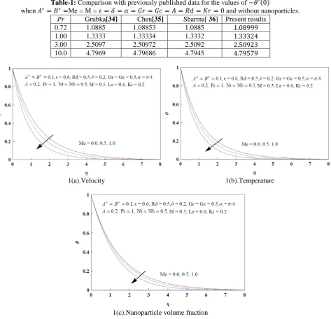
© 2018, IJMA. All Rights Reserved 155 A representative set of graphical results for the velocity, temperature and nanoparticle volume fraction as well as skin friction, local nusselt number and local Sherwood number is present and discuss for different flow parameter values. To verify the accuracy of the results we compared our results with those represented by Grubka [34], Chen [35] & Sharma [36] as shown in table1. The results are in excellent agreement between present and the previous results.

Figure1(a)-1(c) explains the effect of melting parameter Me on velocity, temperature and nanoparticle volume fraction profiles. It is observed that for increasing value of Me the velocity and boundary layer thickness decreases. The temperature distribution decreases with an increasing melting parameter Me. This is because an increasing Me with increasing the intensity of melting, which acts as blowing boundary conditions at the stretching surface and hence tends to thickness the boundary layer. The effect of melting parameters is to reduces the nanoparticle volume fraction profile.

Figures 2 (a)-2(b) depicts the profiles for velocity and temperature for various values of Radiation parameter Rd. It is evident in the figures that an increases Radiation parameter Rd is to enhance velocity and temperature profiles This is due to an increasing the Radiation parameter Rd releases the more heat energy to the flow field. This causes to enhance velocity and thermal boundary layer. In view of this, it concludes that influence of radiation is more significant as 𝑅𝑑 →0(𝑅𝑑 ≠0) and it can be neglect as 𝑅𝑑 → ∞.This agrees the general physical behaviour of the radiation parameter.

The influence of inclined angle on the velocity profile is illustrated in figure (3). It is the fact that as 𝛼= 0 the sheet is in vertical direction and hence maximum gravitational force acts on the flow and when 𝛼=𝜋/2 the sheet is in horizontal direction, the strength of buoyancy forces decreases and hence reduces the velocity boundary layer.

Figure4 (a)-4(c) illustrates the effect of Prandtl number Pr on velocity, temperature and nanoparticle volume fraction. It is seen that the magnitude of the velocity gradient at the surface is higher for higher values of Pr. Thus the velocity field increases with an increase the value of Pr. It is observed that as increasing Pr is leading to decrease the temperature profiles as well as decreases the thermal boundary layer thickness. The nanoparticle volume fraction increases with the increasing Prandtl number value. This is due to the fact that for small values of Pr are equivalent to larger values of thermal conductivities and therefore it is able to diffuse away from the stretching sheet.

Figure 5(a)-5(c) elucidates that when Eyring-Powell parameter(𝜀) increases there is an increase in the velocity profile. Since Eyring-Powell parameter is 𝜀= 1

𝜌𝛽𝑐1𝜈 and =

𝜇

𝜌 . So by increasing Eyring-Powell parameter (𝜀) viscosity of fluid

i.e,𝜇 decreases which causes increasing velocity also fluid becomes less viscous for larger values of Eyring-Powell parameter which enhances fluid velocity. It is noticed that the temperature and nanoparticle volume fraction profiles are decreases with an increasing Eyring-Powell parameter.

Figure 6(a)-6(c) is drawn for the effect of unsteadiness parameter A on velocity temperature and nanoparticle volume fraction profiles. It is clear from the figure that an increasing unsteadiness parameter A reduces the velocity, temperature and nanoparticle volume fraction profiles. At the same time, there is a reduce in the momentum, thermal, concentration boundary layer thickness due to the increasing unsteadiness parameter.

Figure 7 and 8 illustrate the effects of non-uniform heat source/ sink parameters on velocity and temperature profiles. The positive values of 𝐴∗,𝐵∗ heat is generating and releases the heat energy to the flow. Due to this there is an increase in the velocity, temperature profiles with the increase of 𝐴∗,𝐵∗ values.

Figure 9(a)-9(c) shows derivations in velocity, temperature and nanoparticle volume fraction profiles for different values of magnetic field parameter M. When magnetic field strength increases Lorentz force becomes stronger, which creates resistance in the motion of the fluid, so that velocity profile decreases. It is noticed that the temperature and nanoparticle volume fraction profiles are increases with an increasing magnetic field parameter M.

(6)

Figure (12) display the influence of Lewis number Le on nanoparticle volume fraction profile. It is observed from the figure that an increase in the values of Lewis number depreciates the nanoparticle volume fraction and concentration boundary layer thickness decreases. This is due to the fact that mass transfer rate increases.

Figures (13) and (14) depict the variation of thermal Grashof number (Gr) and solutal Grashof number (Gc) on velocity profile. From figures, it is noticed that an increase in the momentum boundary layer thickness and increasing velocity profiles accompanies with an increasing Gr and Gc. The thermal Grashof number Gr signifies the relative effect of the thermal buoyancy force to the viscous hydrodynamic force in the boundary layer as expecting it is noticed that there is a rise in the velocity profile due to the enhancement of thermal buoyancy force. The solutal Grashof number Gc defines the ratio of the species buoyancy force to the viscous hydrodynamic force due to increasing the species buoyancy force there is an increasing the velocity.

Figure(15) shows that the effect of chemical reaction parameter (kr) is to reduces the nanoparticle volume fraction profiles. This is due to the fact that the increasing chemical reaction parameter reduces the concentration boundary layer thickness.

Table-1: Comparison with previously published data for the values of −𝜃′(0)

when 𝐴∗=𝐵∗=Me = M = 𝜀=𝛿=𝛼=𝐺𝑟=𝐺𝑐=𝐴=𝑅𝑑=𝐾𝑟= 0 and without nanoparticles. Pr Grubka[34] Chen[35] Sharma[ 36] Present results

0.72 1.0885 1.08853 1.0885 1.08999 1.00 1.3333 1.33334 1.3332 1.33324 3.00 2.5097 2.50972 2.5092 2.50923 10.0 4.7969 4.79686 4.7945 4.79579

1(a).Velocity 1(b).Temperature

1(c).Nanoparticle volume fraction

(7)

Figure-2: Variation of radiation parameter (Rd) on velocity and temperature profiles

Figure-3: Variation of inclined angle (𝛼)on velocity profile.

4(a) Velocity 4(b) Temperature

4(c) Nanoparticle volume fraction

(8)

5(a).Velocity 5(b) Temperature

Figure-5: Variation of Eyring-Powell fluid parameter (𝜀)on velocity, temperature and nanoparticle volume fraction profiles.

(9)

Figure-7: Variation of non-uniform heat source/sink parameter A*on velocity, temperature profiles

Figure-8: Variation of non-uniform heat source/sink parameter B*on velocity, temperature profiles

(10)

Figure-10: Variation of Thermophoresis parameter (Nt) on velocity, temperature and nanoparticle volume fraction profiles

11(a) Temperature 11(b) Nanoparticle volume fraction

Figure-11: Variation of Brownian motion parameter (Nb) on temperature and nanoparticle volume fraction profiles

(11)

Figure-13: Variation of thermal Grashof number (Gr) on velocity profile

Figure-14: Variation of solutal Grashof number (Gc) on velocity profile

Figure-15: Variation of chemical reaction parameter (Kr)on nanoparticle volume fraction profile

(12)

Table-2: Numerical values of local skin friction coefficient, local Nusselt number and local Sherwood number for different values of𝑀𝑒,𝑅𝑑,𝜀,𝑀,𝐴,𝐾𝑟,𝐴∗,𝐵∗,𝛼,𝑁𝑡,𝑁𝑏,𝐿𝑒.

Me Rd

ε

M A Kr 𝐴∗ 𝐵∗ 𝛼 Nt Nb Le 𝑐_𝑓𝑥 −𝑁𝑢_𝑥 −𝜙′(0)

0.2 1 1 0.2 0.1 0.1 0.1 0.1 0 0.1 0.1 1 −1.937396 1.933218 1.183869

0.4 −2.054798 2.011725 1.239998

0.6 −2.190510 2.102569 1.303912

0.2 1 −1.937396 1.933218 1.183869

2 −1.900713 1.458962 1.293382

3 −1.880101 1.204881 1.347324

1 0.5 −2.218892 1.872103 1.159093

1 −1.937396 1.933218 1.183869

1.5 −1.740928 1.977189 1.201949

1 0.2 −1.553137 1.933218 1.183869

0.4 −1.673683 1.899387 1.170197

0.6 −1.786323 1.867819 1.157600

0.2 0.1 −1.553137 1.933218 1.183869

0.3 −1.654172 2.092968 1.246113

0.5 −1.744609 2.242631 1.281921

0.1 0.1 −1.553137 1.933218 1.183869

0.3 −1.555781 1.930340 1.275106

0.5 −1.557925 1.927988 1.358792

0.1 0.2 −1.548210 1.855707 1.201416

0.4 −1.538307 1.699798 1.236342

0.6 −1.528338 1.542711 1.271031

0.1 0.2 −1.547593 1.849868 1.201992

0.4 −1.533696 1.653739 1.241226

0.6 −1.511522 1.374432 1.287723

0.1 0 −1.553137 1.933218 1.183869

/ 4

π

−1.588180 1.923446 1.179906

/ 3

π

−1.611799 1.916666 1.177178

0 0.1 −1.553137 1.933218 1.183869

0.2 −1.540106 1.917965 0.805071

0.3 −1.527417 1.902698 0.438266

0.1 0.2 −1.557043 1.889365 1.384168

0.4 −1.555871 1.808970 1.481464

0.6 −1.552841 1.733262 1.511536

0.1 1 −1.553137 1.933218 1.183869

2 −1.568682 1.915761 2.041460

3 −1.575631 1.907619 2.703694

4. CONCLUSIONS

This present investigation is a worthwhile attempt to study the problem which involves MHD boundary layer unsteady flow and heat transfer for non-Newtonian Powell-Eyring nanofluid flow past an inclined stretching sheet. The computed results were presented graphically and analyzed the effects of the emerging flow parameters on velocity, temperature and nanoparticle volume fraction profiles and discussed in detail with physical interpretations.

• It is found that effects of the flow parameters M, Me,𝛼, A is to reduces the non-dimensional velocity profile whereas the velocity profile increases with an increase of Rd,

ε

.

• The effect of 𝐴∗,𝐵∗ is to enhances the both velocity and temperature profiles, it is noticed that as A,

ε

increases the temperature and nanoparticle volume fraction profiles decreases as the effect of Pr then reduces the temperature profiles and enhances the velocity and nanoparticle volume fraction profiles.

• The effect of Magnetic field parameter M is to enhance the temperature and nanoparticle volume fraction

profiles, as the effect of Thermophoresis parameter Nt is to enhances the velocity, temperature and

nanoparticle volume fraction profiles, Whereas the nanoparticle volume fraction profiles decrease with the increases of Nb and Le.

• Finally, it is found that the skin friction coefficient value increases with the increase of the values

(13)

decreases with increasing𝑅𝑑,𝑀,𝐾𝑟,𝐴∗,𝐵∗,𝛼,𝑁𝑡,𝑁𝑏,𝐿𝑒.

• It is also seen that mass transfer coefficient value −𝜙′(0) increases with an increasing the values of 𝑀𝑒,𝑅𝑑,𝜀,𝐴,𝐾𝑟,𝐴∗_,_𝐵∗_,_𝑁𝑏_,_𝐿𝑒_{.while decreases with increasing of}_𝑀_,_𝛼_,_𝑁𝑡_.

5. NOMENCLATURE

x distance along the surface y distance normal to the surface u velocity component in x−direction v velocity component in y−direction t time

V velocity field T temperature field

C Nanoparticle volume fraction 𝜏𝑖𝑗 extra stress tensor

p pressure 𝜀,𝛿 fluid parameters 𝜂 local similarity variable 𝑓′ dimensionless velocity 𝜃 dimensionless temperature

𝜙 imensionless Nanoparticle volume fraction 𝛽,𝑐1 material fluid constants

M magnetic parameter Pr Prandtl number Rd Radiation parameter 𝐶𝑓𝑥 local skin friction coeﬃcient

𝑁𝑢𝑥 local Nusselt number

𝑆ℎ𝑥 local Sherwood number

𝑞𝑟 linearized radiative heat flux

𝑘∗_{mean absorption parameter}

𝜎∗_{Stefan-Boltzmann constant}

𝑞′′′ non uniform heat source/sink 𝐴∗_,_𝐵∗_{coefficients of space and temperature} Gr thermal Grashof number

Gc solutal Grashof number Re local Reynolds number

B(t) time-dependent magnetic field 𝐵0 intensity of magnetic field

𝜌 density of fluid 𝜈 kinematic viscosity

𝛼𝑚 effective thermal diffusivity

𝑢𝑚 stretching velocity

𝑇𝑚 surface temperature

𝐶𝑚 surface nanoparticle concentration

𝑇∞ ambient fluid temperature

𝐶∞ ambient fluid concentration

𝐷𝑇 thermophoresis diffusion coefficient

𝐷𝐵 Brownian diffusion coeﬃcient

k thermal conductivity 𝑐𝑝 specific heat capacity

𝑇𝑟𝑒𝑓 reference temperature

𝐶𝑟𝑒𝑓 reference concentration

a positive constant b initial stretching rate 𝑀𝑒 melting parameter Nt thermophoresis parameter Nb Brownian motion parameter Le Lewis number

A unsteadiness parameter 𝜏𝑤 wall shear stress

𝑞𝑤 wall heat flux

𝑞𝑚 wall mass flux

𝜃𝑤 temperature difference parameter

Nr nonlinear thermal radiation parameter Kr chemical reaction parameter

ACKNOWLEDGEMENTS

This research was supported by University Grants Commission-India under Faculty Development Programme. The author gratefully acknowledges the support of UGC.

REFERENCES

1. Crane LJ., Flow past a stretching plate, Z Angrew Math Phys (1970), vol.21, pp.645–647.

2. H.I. Andersson, B.S. Dandapat, Magneto hydrodynamic Flow of a power-law ﬂuid over a stretching sheet,

3. E. Magyari, B. Keller, Exact solutions for self-similar boundary-layer ﬂows induced by permeable stretching walls, Eur. J. Mech. B Fluids (2000) ,vol.19, pp.109–122.

4. Hunegnaw Dessie, Naikoti Kishan, MHD effects on heat transfer over stretching sheet embedded in porous medium with variable viscosity, viscous dissipation and heat source/sink, Ain shams engineering journal(2014),vol.26,pp.967–977.

5. N. Kishan And P. Amrutha, Effects of viscous dissipation on MHD flow with heat and mass transfer over a stretching surface with heat source, thermal stratification and chemical reaction, Journal of Naval Architecture and Marine Engineering (2011), vol.7(1), pp.11–18.

(14)

7. Macha Madhu, Naikoti Kishan,Magneto hydrodynamic mixed convection stagination-point flow of a power-law non-Newtonian nanofluid towards a stretching surface with radiation and heat source/sink, Journal of Fluids(2015),vol.2015,pp.1–14.

8. M Madhu, N Kishan, Finite element analysis of heat and mass transfer by MHD mixed convection stagnation-point flow of a non-Newtonian power-law nanofluid towards a stretching surface with radiation, Journal of the Egyptian Mathematical Society(2016), vol.24(3), pp.458–470.

9. M Madhu, N Kishan, A Chamka, Boundary layer flow and heat transfer of a non-Newtonian nanofluid over a non-linearly stretching sheet, International Journal of Numerical Methods for Heat & Fluid Flow(2016),vol.26(7),pp.2198–2217.

10. M Madhu, N Kishan, MHD boundary-layer flow of a non-Newtonian nanofluid past a stretching sheet with a heat source/sink, Journal of Applied Mechanics and Technical Physics(2016),vol.57 (5), pp.908–915.

11. M. Patel, M.G. Timol, Numerical treatment of Powell-Eyring ﬂuid ﬂow using method of satisfaction of asymptotic boundary conditions, Appl. Numer. Math.(2009),vol.59 pp.2584– 2592.

12. T. Hayat, Z. Iqbal, M. Qasim, S. Obidat, Steady ﬂow of an Eyring Powell ﬂuid over a moving surface with convective boundary conditions, Int. J. Heat Mass Transf.(2012), vol.55 pp.1817– 1822.

13. A.V. Rosca, I.M. Pop, Flow and heat transfer of Powell-Eyring ﬂuid over a shrinking surface in a parallel free stream, Int. J. Heat Mass Transf.(2014), vol.71,pp.321–327.

14. M. Jalil, S. Asghar, S.M. Imran, Self similar solutions for the ﬂow and heat transfer of Powell -Eyring ﬂuid over a moving surface in a parallel free stream, Int. J. Heat Mass Transf. (2013), vol.65,pp.73–79.

15. S. Islam, A. Shah, C.Y. Zhou, I. Ali, Homotopy perturbation analysis of slider bearing with Powell-Eyring fluid, Z. Angew. Math. Phys (2009),vol. 60,pp.1178–1193.

16. V. Sirohi, M.G. Timol, N.L. Kalathia, Numerical treatment of Powell-Eyring fluid flow past a 90 degree wedge, Reg. J. Energy Heat Mass Tran(1984) ,vol.6(3), pp.219–228.

17. R.E. Powell, H. Eyring, Mechanism for relaxation theory of viscosity, Nature(1944) vol.154,pp.427–428. 18. T. Hayat, Z. Iqbal, M. Qasim, S. Obaidat, Steady flow of an Eyring-Powell fluid over a moving surface with

convective boundary conditions, Int. J. Heat Mass Transf.(2012) vol.55, pp.1817–1822.

19. S.U.S. Choi, J.A. Eastman, Enhancing thermal conductivity of fluids with nanoparticles, ASME Pub. Fed. (1995), Vol.231, pp.99–106.

20. W.A.Khan, I.Pop, Boundary-layer flow of a nanofluid past a stretching sheet, Int. J. Heat Mass Transf.(2010), vol.53, Pp .2477-2483.

21. Kuznetsov VA and Nield D A,

International Journal of Thermal Sciences, (2010), vol.49(2), pp.243–247.

22. Transient response behavior of an axisymmetric stagnation flow on a circular cylinder due to time dependent free stream velocity,

23. Rajesh Vemula, Lokenath Debnath, Sridevi Chakrala, Unsteady mhd Free convection flow of nanofluid past an accelerated vertical plate with variable temperature and thermal radiation,

24. Casson Fluid Flow over an

Unsteady Stretching Surface, Ain Shams Engineering Journal(2013), Vol. 4(4), pp. 933-938.

25. L. Roberts, On the melting of a semi-infinite body of ice placed in a hot stream of air, J. Fluid Mech.(1958), vol.4, pp.505-528.

26. T. Hayat, M. Farooq, and A. Alsaedi, Melting heat transfer in the stagnation point flow of Maxwell fluid with doublediffusive convection, Int. J. Numer. Methods Heat Fluid Flow(2014). vol.24, pp.760–774.

27. K. Das, Radiation and melting effects on MHD boundary layer flow over a moving surface, Ain Shams Eng. J.(2014), vol.5, pp.1207–1214.

28. E.M. Epstein, D.H. Cho, Melting heat transfer in steady laminar flow over a flat plate, J. Heat Transfer (1976), vol.98, pp.531-533.

29. M. Kazmierczak, D. Poulikakos, I. Pop, Melting from a flat plate embedded in a porous medium in the presence of steady convection, Numer. Heat Transfer (1986), vol.10, pp.571-581.

30. R.S.R.Gorla, M.A. Mansour, I.A. Hussanien, A.Y. Bakier, Mixed convection effect on melting from a vertical plate, Transport Porous Med.(1999) ,vol.36,pp.245-254.

31. N. Bachock, A. Ishak, I. Pop, Melting heat transfer in boundary layer stagnation point flow towards a stretching/shrinking sheet, Phys. Lett. A(2010), vol.374,pp.4075-4079.

32. A.J. Chamkha, A.M. Rashad, E. Al-Meshaiei, Melting effect on unsteady hydrodynamic flow of a nanofluid past a stretching sheet, Int. J. Chem. React. Eng. (2011), vol.9. Pp.1-13.

33. R.S.R. Gorla, A. Chamkha, A. Aloraier, Melting heat transfer in a nanofluid flow past a permeable continuous moving surface, J. Nav. Arch. Mar. Eng.(2011), vol.2, pp.83-92.

34.

35.

(15)

transfer past a stretching surface embedded in a porous medium using element free Galerkin method

37. I.S. Oyelakin, S. Mondal, P. Sibanda, Unsteady Casson nanofluid flow over a stretching sheet with thermal radiation, convective and slip boundary conditions, Alex. Eng. J. 55 (2016) 1025–1035.

38. P. Mohan Krishna, N. Sandeep, J. V. Ramana Reddy and V. Sugunamma, Dual solutions for unsteady flow of Powell Eyring fluid past an inclined stretching sheet, Journal of Naval Architecture and Marine Engineering (2016), vol.13 (1), pp. 89-99.