Vol 7, No 8 (2017)

(1)

Research Article

August

2017

Computer Science and Software Engineering

ISSN: 2277-128X (Volume-7, Issue-8)

Brain Tumor Segmentation from Multi-Spectral Images

Using Multi-Kernel Learning

Naouel Boughattas* Maxime Berar Kamel Hamrouni Su Ruan

Electric Dep &Tunis-Elmanar Physics Dep & Rouen Electric Dep & Tunis-Elmanar Medecine Dep & Rouen Tunisia France Tunisia France

DOI: 10.23956/ijarcsse/V6I2/01212

Abstract— We propose a brain tumor segmentation method from multi-spectral MRI images. The new idea is to use Multiple Kernel Learnin (MKL) which jointly selects one or more kernels associated to each feature and trains SVM (Support Vector Machine).

First, a large set of features based on wavelet decomposition is computed on a small number of voxels for all types of images, allowing us to build a training feature base. The segmentation task is then viewed as a learning problem where only the most significant features from the feature base are selected and a classifier is then learned. The images are then segmented using the trained classifier on the selected features.

Our algorithm was tested on the real data provided by the challenge of Brats 2012. The dataset includes 20 high-grade glioma patients and 10 low-grade glioma patients. For each patient, T1, T2, FLAIR, and post-Gadolinium T1 MR images are available. Our algorithm was compared to the resulting top methods of the challenge of Brats 2012. The results show good performances of our method.

Keywords— Cerebral MRI, tumor, segmentation, feature selection, multiclass, classification, multiple kernel learning, multimodal.

I. INTRODUCTION

Brain tumor segmentation consists in partitioning the different tumor tissues from normal brain tissues. Fast and accurate segmentation of brain tumor images is an important but difficult task in many clinical applications such as radiotherapy or surgical planning. As it provides a good soft tissue contrast, Magnetic Resonance Imaging (MRI) is currently the standard technique for brain tumor diagnostic (see for example the surveys by Bauer[1], Gordillo[2] or El-Sayed[3]). MRI can also produce different types of tissue contrasts by varying excitation and repetition times, enhancing different aspects of the tissues and revealing different subregions of the tumor such as necrotic, active or edema subregions. Despite continuous advances in imagery technology, brain tumors, owing to their extremely heterogeneous shapes, appearances and locations still present a serious challenge to segmentation techniques.

Over the past years [4], machine learning methods have been more and more used to deal with brain segmentation [1]. There are two types of methods: supervised or unsupervised [5]. In unsupervised methods, the aim is to aggregate the pixels in clusters depending on a given criterion, without any a priori information or label on pixels. The Expectation-Maximization algorithm, the Markov Random Field method and the Gaussian Mixture Model are learning methods from this category, which have all been used in brain tumors segmentation schemes as seen in works by Farzinfar et al.[6], Zhang et al.[7], Ji et al.[8] or Dong et al. [9]. Moreover, these techniques can be used for genuine brain images analysis. In contrast, segmentation methods integrating supervised learning use prior information given by the radiologist on a small set of pixels in order to learn a classifier, which will be then used to label the unlabeled pixels, thus segmenting the whole image volume. This kind of segmentation methods uses various learning techniques, such as Support Vector Machines (SVM) [10], random forests [11, 12] and Bayesian classifier [13]. A classification forest combined with context information and initial probability estimated for the single tissue classes topped the challenge of BraTS 2012 [14].

(2)

ISSN(E): 2277-128X, ISSN(P): 2277-6451, DOI: 10.23956/ijarcsse/V6I2/01212, pp. 10-16

In this paper, we propose a brain tumor segmentation method from MRI multi-sequence. First, a large set of features based on wavelet coefficients is computed on all types of images from a small number of voxels, allowing us to build a training feature base. The segmentation task can be considered as a learning problem where only the most significant features from the feature base are selected. The new idea is to use MKL by associating one or more kernels to each feature in order to solve jointly the two problems: (1) selection of the features and their corresponding kernels, (2) training of the classifier. The tumor and edema are then segmented using the trained classifier on the selected features extracted from the whole image volumes. Finally, a post-processing step, based on morphological operations, is performed.

In order to compare with different state-of-the-art methods, we have tested our method using the database provided by the Multimodal Brain Tumor Segmentation (BraTS) 2012 challenge [14]. It is a large dataset of brain tumor MR scans in which the tumor and edema regions have been manually delineated and been made available to the public. Methods based on random forests [11, 12] have topped the challenge, but as shown by our results on the same database, our method is also competitive.

The paper is organized as follows: The next section of this paper is devoted to our method and its different steps, including a brief presentation of the MKL. Then, we compare our results with those best methods of the MICCAI 2012 BraTS [14] challenge on real data. We conclude finally.

II. METHOD

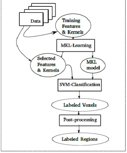
Our method is classically divided into three steps: a learning step, a classification step and a post-processing step as seen Fig. 1. The learning step is composed of two stages: an extraction of associated features and a MKL training. Features are first extracted from a small set of voxels labelled by experts and then selected by MKL method which uses a sparsity constraint. The parameters and hyperparameters of the MKL are estimated in this learning step. Therefore no manually trade-off of these parameters is necessary. The classification is then performed on all the voxels of all images using only the selected features to obtain three classes: edema, tumor or healthy tissues. Finally, the post-processing step corrects some false classification on the segmented regions and their peripheries.

Fig. 1 Proposed framework of our method.

A. Feature Extraction

In the literature, numerous features can be extracted to describe brain tumor texture in MR images. Intensity based features [18], such as mean, variance, and median characterize the grey level of the tumor. Texture based features, such as LBP [19], wavelet coefficients [18] allow to identify different textural patterns in tumor areas and health tissues.

In our experiments, the training points are selected as follows: for each patient, the practician is asked to roughly delineate the tumor boundary, the edema boundary and a small healthy zone on only one slice in one modality of the same patient. Sampling voxels as centers of the features patches in the three regions allow us to generate training sets per class. The number of voxels samples to train the classifiers has been empirically set to 150 samples per class.

B. MKL training

(3)

SVM with this new kernel could be used to classify. The best classification is obtained when the best combination of the kernels is found.

Introduced by Lanckriet et al. in [17], multiple kernel learning methods have been developed to determine the positive weight

d

_m associated to each kernel

k

_m. In a MKL-SVM framework, the decision function has the following form:

1 1

( )

(

,

)

p l

m m i m m i i m

f x



d k

x

 





(1)

where the



_i are the weights associated to each training example

x

_i of label

y

_i and

x

_im and

x

mrepresents the feature associated to kernel

k

_m. If f(x) > 0, the corresponding point is associated to class 1, otherwise class 0.

We can associate each kernel weight to a single kernel applied to one feature. By applying a sparsity constraint on the kernel weights, it will allow us to select both the informative features and adapted kernels. In practice, it allows us to utilize several kernels of the same family with different parametrizations.

Numerous methods and formulations exist for solving the MKL problem in literature, mostly in bi-class settings. Our experimental setting (healthy tissues, edema, tumor) is multiclass setting and any of the bi-class method could be used in a one-against-all strategy. However, in this case there will be as many kernel weights determined as classes. We chose the SimpleMKL algorithm [20] in our method mainly because a version is provided for multi-class settings using a common kernel weights determination for all classes. It will enable a better interpretation of the selected kernels. The SimpleMKL algorithm is based on solving the primal problem using a simple gradient method. The primal problem determines jointly the kernel functions

f

_m, the kernel weights

d

_mand the soft margin parameters



_i:

{ } , ,

1 min

2

. . ( ) 1 , 0, ,

1, 0, .

n m

m m i

f d

m i

i m i i i

m

m m

m

d f C

s t y f x i

d d m

 

 

   

  



(2)

The l₁normsparsity constraint on the positive weights

d

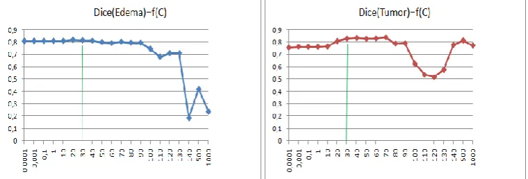
m is given by fixing their sum equal to one. The

regularisation hyperparameter C is adjusted in a fully automatic way by initializing with a very small value and then incremented regularly. Observed on a bi-class problem, increasing C results on growing tumor regions because the regularisation term makes more and more points to be classified to the tumor. It exists an interval of C-value, where segmented regions are stable, corresponding to stable kernel weights. On a multi-class problem, the stability of the segmented region is less observable, but there is still an interval of C-value, corresponding to stable kernel weights. The adopted validation strategy is then: once the variations of kernel weights become lower than a given threshold

( )



i , the

current value of C is chosen. Fig. 2 shows the chosen value of C (C = 30) for the patient HG03, which is within a stability field and near the maximal Dice score.

Fig. 2 Dice scores of edema (left) and tumor (right) segmentation for the patient HG0003. The abscissa denotes the C value and the ordinate indicates the Dice score value.

C. MKL based SVM classification and post-processing step

Once the regularization parameter C is chosen, the MKL-SVM algorithm can be applied on all voxels of the patient volumes using the non-null kernel weights

d

_m and coefficients



_i computed from the previous learning step using equation (1). Indeed, the values of

d

_m define if the corresponding features are selected. If

d

_m = 0, the corresponding feature is not selected. Thanks to the training step and the sparse constraint, we use only a small subset of features associated to the chosen kernels (with non-null weights) to classify the voxels. That allows to decrease classification time and increase the classification performance.

(4)

III. MATERIAL AND RESULTS

A. Material

We evaluate our approach on real patients MRI of the dataset of the MICCAI 2012 BraTS challenge: 20 high-grade glioma patients, where tumor tissues and healthy tissues are well differentiated, and 10 low-grade glioma patients, where tumor tissues and healthy tissues are poorly differentiated, both with and without resection, along with expert annotations for active tumor and edema. For each patient, T1, T2, FLAIR, and post-Gadolinium T1 MR images are available as seen in Fig. 3. All volumes were linearly co-registered to the T1 contrast images, skull stripped, and interpolated to 1mm isotropic resolution. The MR scans are provided as well as the corresponding reference segmentations.

Fig. 3 Slices of the four volumes of a patient (from left to right: post-Gadolinium T1, T1-weighted, T2-weighted and Flair)

B. Experiments & Results

In this paper, we used a set of features based on Multilevel 2-D Discrete wavelet decomposition calculated on a patch surrounding each labeled voxel, as feature for brain tumor description in MR images [18]. The whole feature set is composed of nine different details and one residual coefficients of Haar 2D wavelet decomposition calculated separately on each modality, combined through Gaussian kernels with different parameters defined as the standard deviation of the feature multiplied by factors 0.1,1 or 10. It results on 120 kernels.

For each patient, we can provide the evaluation results corresponding to the segmentations obtained by the MKL learning. We will also present as a control experiment the dice score of the segmentation given by the most-weighted kernel of the MKL. Ideally, the MKL learning results should perform better than any single kernel of the MKL kernel set. The dice score is computed using the on-line tool available during the challenge.

1) Results for High-Glioma patients

Table I Detailed MKL-SVM segmentation results of high-grade gliomas patients in the BRATS dataset. Dice score is reported for the segmentation of edema (E) and active tumor (T).

Volume MKL-SVM Best kernel

E T E T

HG01 0.62 0.60 0.60 0.46 HG02 0.74 0.51 0.52 0.34 HG03 0.82 0.84 0.39 0.74 HG04 0.52 0.69 0.46 0.54 HG05 0.47 0.33 0.08 0.20 HG06 0.45 0.59 0.34 0.52 HG07 0.53 0.60 0.50 0.44 HG08 0.71 0.68 0.27 0.51 HG09 0.68 0.71 0.63 0.59 HG10 0.39 0.59 0.29 0.08 HG11 0.77 0.87 0.45 0.68 HG12 0.42 0.61 0.27 0.10 HG13 0.59 0.70 0.47 0.68 HG14 0.24 0.52 0.28 0.58 HG15 0.78 0.87 0.34 0.78 HG22 0.66 0.41 0.65 0.17 HG24 0.62 0.71 0.38 0.19 HG25 0.51 0.55 0.08 0.20 HG26 0.71 0.50 0.41 0.14 HG27 0.67 0.80 0.55 0.55 mean 0.60 0.63 0.40 0.42

min 0.24 0.33 0.08 0.08

(5)

Table I details the Dice scores for the high-grade patients of the datatset. We compare results of our method as well as the results given by the single best kernel. It can be observed that the results using the best single kernel in the control experiment are worse than the results obtained by the proposed method, except for patient HG14. In this case, the results of our method and the control experiment are similar. Fig. 4 shows an example of segmentation results for one high gliomas patient (HG27).

Fig. 4 Examples of segmentations for one slide of Patient HG27.

Left : edema region, Right: tumor region, Green : True Positives, Blue : False Negatives and Yellow : False Positives.

2) Results for Low-Glioma patients

Table II details the Dice scores for the low-grade patients of the dataset obtained at each step of the method as well as the results given by the single best kernel control experiment. Our learning step is not as effective as the control experiment for three patients out of 10. These results are less globally satisfying than the results for High-grade patients, because the quality of images is not as good as for high grade patients.

Table II Detailed MKL-SVM segmentation results of low-grade gliomas patients in the BRATS dataset. Dice score is reported for the segmentation of edema (E) and active tumor (T).

Volume MKL-SVM Best kernel

E T E T

LG01 0.29 0.26 0.28 0.36 LG02 0.71 0.73 0.71 0.69 LG04 0.60 0.64 0.42 0.26 LG06 0.67 0.54 0.24 0.52 LG08 0.58 0.69 0.59 0.44 LG11 0.41 0.86 0.44 0.85 LG12 0.51 0.66 0.53 0.70 LG13 0.43 0.69 0.13 0.32 LG14 0.15 0.46 0.15 0.52 LG15 0.60 0.78 0.15 0.73 mean 0.49 0.63 0.36 0.54

min 0.15 0.26 0.13 0.26

max 0.71 0.78 0.71 0.85

3) Influence of the number of learning voxels

Given a fixed value of the regularisation parameter C, let us study the influence of the size of the learning set to the Dice score value and to the learning time. Table III shows the Dice score values as well as the learning time under different size of learning sets. From Table III, it can be observed that the Dice score as well as the learning time increase with the increasing of the learning set. With the best value of dice score and a reasonable learning time, the chosen size of the learning set is 150 points.

Table III Inuence of increasing the number of learning points: Dice score values and learning step duration for Patient HG0003.

Number of training voxels

Learning duration (sec.)

Dice scores (Edema/Tumor)

(6)

90 points 2.44 0.80 / 0.81 120 points 3.31 0.81 / 0.81 150 points 3.96 0.82 / 0.84 180 points 5.57 0.82 / 0.84

4) Discussion

Table IV Detailed comparison our MKL-SVM results with those of the methods from the challenge of MICCAI 2012 (Dice score)

Volume HG LG Mean

E T E T

MKL-SVM 0.58 0.65 0.48 0.64 0.60 Zikic [11] 0.70 0.71 0.44 0.62 0.62

Bauer [10] 0.61 0.62 0.35 0.49 0.52 Hamamci [21] 0.56 0.73 0.38 0.71 0.60 Geremia [12] 0.56 0.58 0.29 0.20 0.41 Zhao [14] - - - - 0.33 Subbanna [14] - - - - 0.615 Fernandez [14] - - - - 0.49 Menze[14] 0.57 0.56 0.42 0.24 0.45 Menze[14] 0.70 0.71 0.49 0.23 0.54 Riklin[14] 0.61 0.59 0.36 0.32 0.52

In order to evaluate the performance of the proposed method, we use the mean Dice scores to compare our segmentation results with those of participating methods of the challenge BRATS 2012. This comparison is shown in Table IV. The winning methods of the challenge were: Zikic et al. [11], Bauer et al. [10] and Hamamci et al. [21]. Only Hamamci et al. don't use classification based on features extracted from all modalities. Compared with these three methods, only the method of Zikic et al. [11] performs better than ours. Among all the other methods of the challenge, only that of Subbana et al. [14] performs slightly better than us. The methods presented by Zikic et al. [11] and Geremia et al. [12] use forest classification. The method of Bauer et al. [10] rep ²laced a SVM judged less sophisticate used in a previous version of their method by a random forest classification. In [14], Subbanna et al. used a Bayesian classifier. However, for all those methods the classification step is either completed by a priori information learned on other patients such as tissue-specific intensity based models [11] or regularized via a Conditional Random Field [10], while our method uses a very simple training process. From Table IV, we can see that our method performs better in edema segmentation for low-grade dataset than the winning methods of the challenge.

IV. CONCLUSION

A segmentation system for brain tumor from multi-spectral MRI images is presented in this paper. This system is based on a MKL-SVM algorithm to deal with multi-input data and to solve challenging tumor segmentation problem. The system allows to automatically select multiple kernels to each feature based on wavelet coefficients, to exploit the diversity and the complementarity of all used data and selects automatically the most significant ones thanks to a sparsity constraint posed on kernel weights. The sparsity constraint favours the selection of informative feature. Our MKL-SVM algorithm is followed by a post-processing step based on morphological operations. Our method is compared with other methods participating to the challenge of MICCAI BRATS 2012. This comparison shows that the proposed method gives competitive results especially for low-grade patients.

In future works we would like to extend our training on 3D volumes, to test different MKL implementation, to involve more diverse feature and kernels and to compare on brain tumor datasets labelled with many classes.

REFERENCES

[1] Bauer, S., Wiest, R., Nolte, L.P., Reyes, M.. “A survey of mri-based medical image analysis for brain tumor studies”. Physics in Medicine and Biology 2013;58(13):R97.

[2] Gordillo, N., Montseny, E., Sobrevilla, P.. “State of the art survey on {MRI} brain tumor segmentation. Magnetic Resonance Imaging ”.2013;31(8):1426 - 1438.

[3] El-Dahshan, E.A., Mohsen, H.M., Revett, K., Salem, A.M.. “Computer-aided diagnosis of human brain tumor through MRI: A survey and a new algorithm”. Expert Syst Appl 2014;41(11).

[4] Schad, L.R., Bluml, S., Zuna, I.. “Mr tissue characterization of intracranial tumors by means of texture analysis”.

Magnetic Resonance Imaging1993;11(6):889 - 896.

[5] Hastie, T., Tibshirani, R., Friedman, J.. “The Elements of Statistical Learning”. Springer Series in Statistics; New York, NY, USA: Springer New York Inc.; 2001.

(7)

[7] Zhang, T., Xia, Y., Feng, D.D.. “Hidden markov random field model based brain {MR} image segmentation using clonal selection algorithm and markov chain monte carlo method”. Biomedical Signal Processing and

Control 2014;12(0):10 - 18.

[8] Ji, Z., Xia, Y., Sun, Q., Chen, Q., Feng, D.. “Adaptive scale fuzzy local gaussian mixture model for brain MR image segmentation”. Neurocomputing 2014;134:60 - 69.

[9] Dong, F., Peng, J.. “Brain MR image segmentation based on local gaussian mixture model and nonlocal spatial regularization”. J Visual Communication and Image Representation 2014;25(5):827 - 839.

[10] Bauer, S., Nolte, L.P., Reyes, M.. “Fully automatic segmentation of brain tumor images using support vector machine classification in combination with hierarchical conditional random field regularization”. Medical Image

Computing and Computer-Assisted Intervention-MICCAI 2011 :354-361.

[11] Zikic, D., Glocker, B., Konukoglu, E., Criminisi, A., Demiralp, C., Shotton, J., et al. “Decision forests for tissue-specific segmentation of high-grade gliomas in multi-channel mr”. Medical Image Computing and

Computer-Assisted Intervention-MICCAI 2012. Springer Berlin Heidelberg; 2012, p. 369-376.

[12] Geremia, E., Clatz, O., Menze, B., Konukoglu, E., Criminisi, A., Ayache, N.. “Spatial decision forests for ms lesion segmentation in multi-channel magnetic resonance images”. NeuroImage 2011;57(2):378-390.

[13] Corso, J., Sharon, E., Dube, S., El-Saden, S., Sinha, U., Yuille, A.. “Efficient multilevel brain tumor segmentation with integrated bayesian model classification”. Medical Imaging, IEEE Transactions on 2008;27(5):629-640.

[14] Menze, B., Jakab, A., Bauer, S., Prastawa, M., Reyes, M., Van Leem-put, K.. “The Multimodal Brain Tumor Image Segmentation Benchmark (BRATS) ”. Tech. Rep, 2012.

[15] Chen, X.w., Wasikowski, M.. Fast: “A roc-based feature selection metric for small samples and imbalanced data classification problems”. In: Proceedings of the 14th ACM SIGKDD International Conference on Knowledge

Discovery and Data Mining. KDD '08; New York, NY, USA: ACM. ISBN 978-1-60558-193-4; 2008, p.

124-132.

[16] Wang, L.. “Feature selection with kernel class separability”. Pattern Analysis and Machine Intelligence, IEEE

Transactions on 2008;30(9):1534- 1546.

[17] Lanckriet, G.R., Cristianini, N., Bartlett, P., Ghaoui, L.E., Jordan, M.I.. “Learning the kernel matrix with semidefinite programming”. The Journal of Machine Learning Research 2004;5:27-72.

[18] Zhang, N., Ruan, S., Lebonvallet, S., Liao, Q., Zhu, Y.. “Kernel feature selection to fuse multi-spectral mri images for brain tumor segmentation”. Computer Vision and Image Understanding 2011;115(2):256 - 269. [19] Ojala, T., Pietikainen, M., Maenpaa, T.. “Multiresolution gray-scale and rotation invariant texture classification

with local binary patterns”. Pattern Analysis and Machine Intelligence, IEEE Transactions on 2002;24(7):971- 987.

[20] Rakotomamonjy, A., Bach, F., Canu, S., Grandvalet, Y.. “Simplemkl”. Journal of Machine Learning Research 2008;9(11).