Definition of an active deformation model for manipulation of flexible objects

(1)

Master ARIA - ROBA

Thesis Report

Definition of an active

deformation model for

manipulation of flexible objects

Author:

Vyshakh

_{Palli Thazha}

Supervisors:

S´ebastien

_Briot

Abdelhamid

_Chriette

Philippe

_Martinet

President:

Olivier

_Kermorgant

(2)

List of Figures

1 Different categories of deformable object modeling - Adopted from

[16] . . . 10

2 Indirect positioning of deformable objects adopted from [23] . . . 11

3 Spring model of deformable object [23] . . . 12

4 Classification of mesh points adopted from [23] . . . 12

5 Flow of control method adopted from [23] . . . 13

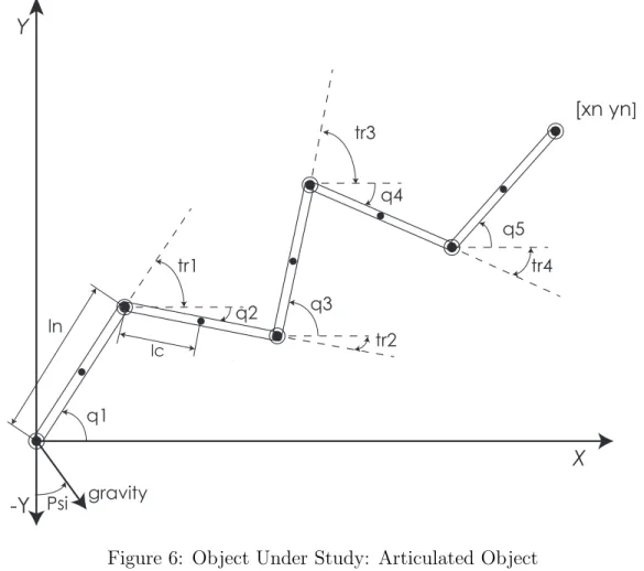
6 Object Under Study: Articulated Object . . . 15

7 Error plot for the potential function . . . 19

8 Error plot for the potential function for object with 4 links . . . 22

9 Configuration space of the object . . . 24

10 Configuration space of a 4 link object . . . 25

13 Configuration space represented as a grid map . . . 27

14 Increments of square areas . . . 30

15 Representation of the trajectory . . . 31

16 Representation of the trajectory (Zoomed) . . . 31

17 Choosing Start and End Configurations from the Configuration Space 32 18 Trajectory generated for 4-link object shown in blue . . . 33

19 Trajectory generated for 4-link object shown in blue . . . 34

20 Configuration Space for different gravity angles Psi . . . 36

21 Configuration Space for a gravity angle of 4π/10 . . . 37

22 Configuration Space for a gravity angle of 6π/10 . . . 37

23 Configuration Space for a gravity angle of 4π/10 (Zoomed) . . . 38

24 Configuration Space for a gravity angle of 6π/10 (Zoomed) . . . 38

25 Dexterous manipulation Setup for 3-link object with two 2R planar robots . . . 43

26 Dexterous manipulation Setup for 4-link object with two 2R planar robots . . . 43

27 Error Propagation for First Task T1 - G1 = 3; G2 = 0.3 . . . 46

28 Error Propagation for Second Task T2-G1 = 3; G2 = 0.3 . . . 46

29 Error Propagation for first task T1 when gain G1 is changed . . . 47

30 Error Propagation for Second task T2 when gain G1 is changed . . . . 48

(5)

38 Apdaptive gain G1 . . . 52

39 Error Propagation for First task T1 for trajectory of 4-link object . . 52

40 Error Propagation for First task T2 for trajectory of 4-link object . . 53

41 Error Propagation for First taskT1 with adaptive gainG1 - four link

object . . . 53

(6)

1 Acknowledgments

The research described in this thesis was carried out from November 2015 to July 2016 as a part of the Robotics (ARMEN) team of the ”Institut de Recherche en

Com-munications et Cybern´etique de Nantes” (IRCCyN) in Nantes. The robotics

mas-ter was financially supported by the European Union, under theErasmus Mundus

program calledInterweave.

First of all, I am deeply indebted to my supervisor Professor S´ebastien BRIOT

for pushing and motivating me to produce results even when I was going through

a tough time, my co-supervisors Professor Philippe MARTINET, and Professor

Abdelhamid CHRIETTE for their encouragement, valuable advises, continuous and indispensable assistance, and their great help. I would like to thank them for their helpful guidance and great care. The numerous discussions and the motivating investment in the research surrounding my thesis is more than greatly appreciated. It is really my pride to perform my Masters research thesis under their supervision.

I would like also to express my gratitude to Professor Olivier KERMORGANT

to have honored me for presiding the jury and for his suggestions allowing me to enforce certain perspectives in my research subject. Also I would like to thank

Pro-fessorIna TARALOVAfor her suggestions and critical remarks on my work which

helped me improve my report and the work that was put into it.

I would like to thank my colleagues who have, all throughout my thesis, helped with various aspects of my work and for supporting me to succeed in the whole research experience and enjoying it at the same time.

I would like to deeply thank my friends in Nantes, and around Europe, especially from University of Genoa and from around the world for the unforgettable moments we spent together. Finally, I owe a huge debt of gratitude and sincere thanks to my parents and family, they have lost a lot due to my research abroad. Without their encouragement and support it would have been impossible for me to finish this work. Thank you.

(7)

2 Abbreviations

MRI - Magnetic resonance imaging

CT - Computed Tomography

NURBS - Non Uniform Rational B-Splines

DoF - Degrees of Freedom

FEM - Finite Element Method

BEM - Boundary Element Method

CV - Computer Vision

CoM - Center of Mass

A* - A-Star

(8)

3 Abstract

Manipulation of flexible objects plays an important rule in the industry. Any in-dustry that involves the use of a deformable object will, at one certain point of time, require robots to handle these objects. Be it handling of food items in the food industry, folding or sorting of clothes in the textile industry, or handling of cables in various industries etc.. every where there arises a need to study how these objects could be manipulated. So modeling of objects has to be studied, using the developed model to plan trajectories and motions for a robot to handle this object has to be studies, vision based control to correctly manipulate the object using the developed motion planning strategies has to be developed. This master thesis is a first step into the study of an articulated object and its manipulation.

The modeling of the object is studied which is used to find the equilibrium config-urations and hence the configuration space of the object. The configuration space is studied and path planning algorithms are used to generate trajectories from one equilibrium configuration to another.

The manipulation of the object using two 2R planar robots is studied. For this, task-priority based control of redundant manipulators is studies and implemented. Simulations and results are documented.

(9)

4 Introduction

4.1 Topic of Research

Robots and robotic technologies have been evolving at a fast pace over the past few decades and there is a wide range of robots specialized for different application like manipulation, navigation, surveillance, rescue, medical treatment and the list goes on. Manipulation of real world objects has been an important area of research for years and robots which can manipulate rigid objects are very common in indus-tries around the globe. Increased productivity, lowered cost and better precision is obtained by using robots. But when it comes to manipulation of soft or flexible objects, the robots are still not capable enough and the technologies which enable to manipulate a soft object with the dexterity of a human hand is still to be de-veloped. Because of this inability of perfect manipulation, the research topic of developing the perfect technology for doing the same has been picking up pace and is a hot topic for developments at this point of time. Several methods have been proposed which try to solve this and although many of them succeed in its own way, they have their own drawback making their application to a wide variety of objects impossible. Some methods even though provides good results are computationally expensive while some others have some other constraints.

Deformable objects are found in a wide range of industries like food industry, garments, packaging, manufacturing, industries involving elastic objects and the list goes on. Deformable objects are hard to manipulate because of their low stiffness and they are susceptible to large deformations on application of force. They change their shape and volume during handling. Thus a static model of the object cannot be used like in the cases of rigid objects. Model based and model-free methods have been studied for manipulation of deformable objects. The state of the art will be detailed in the coming sections.

(10)

4.2 Organization of the report

The rest of the report is organized as follows. In Section 4.3, the general techniques that are used to model deformable objects are specified. In Section 4.4, the state of the art in deformable object manipulation is discussed. In Section 5 the object that is studied is described and elaborated. In Section 6 the modeling of the already defined object and Lagrange formulations of modeling is elaborated. In Section 7 and Section 8, the modeling technique is extended to objected with 3 and 4 connected links respectively. In Section 9 the configuration space of the modeled object is defined and in section 10 the configuration space is represented as a grid map. In Section 11, trajectory generation techniques are studied and applied to the object

manipulation. Shortest path algorithms like A-star algorithm and Probabilistic

Roadmap Method is elaborated. In Section 12 the effect on gravity angle to the equilibrium state of the object is studied. In Section 13 the modeling of robots, redundant manipulation and application of 2R robots for manipulating the proposed object is studied. In Section 14 a task-priority approach for redundant manipulators is studied and results are plotted for different conditions and gains are tuned.

(11)

4.3 Modeling of deformable objects

Deformable objects can be one modeled either in one dimension (lines and curves), two dimensions (surfaces) or three dimensions (solid objects). These models are used for different applications such as animations, image segmentation, 3D reconstruction of bones and organs from MRI or CT scans, haptics, mechanical simulations, surgery planning etc. [16]

All these applications are diverse and the utilization of one single modeling method for all these is not appropriate and over the years a variety of methods have been developed and implemented for the same. The deformable models can be classified into three categories. Heuristic methods, Continuum-mechanical models, and hybrid methods which combine both the previous categories.

Figure 1: Different categories of deformable object modeling - Adopted from [16] The heuristic approaches use straightforward techniques of geometry of the de-formable objects including their elastic properties. In the beginning these methods used to model solid objects as hollow shells because most of the applications focused on deformation on the surface level. This reduced the size to less than a hundredth of its initial size. But this approximation neglects the conservation of its volume. So later, methods like springmass models were extended to include changes in volume -linked volume algorithms, tensor-mass model which used tetrahedral elements were developed.

The continuum-mechanical approaches are more exact but they are far too complex and computationally costly. This category has methods like Finite Element method (FEM) which involves a discretization of the entire object and Boundary Element

(12)

(BEM) approach which maps the calculations of the interior of the object to its surface, thereby requiring discretization of only the surface.

The hybrid approach divides the object into parts and finds the best possible ap-proach for each part bases on how this part is interacted with.

4.4 Manipulation of Deformable objects

A successful attempt of manipulating deformable object using indirect positioning is presented in [23]. They use a crude model of the system and a robust control system to nullify the inadequacies of the model.

Figure 2: Indirect positioning of deformable objects adopted from [23] Model is made for two dimensional objects by discretizing into mesh-points and each mesh point being connected by horizontal, vertical and diagonal springs as shown in Fig.3. The model describes translation, orientation and deformation of the

object. Position vector of the (i, j)-th mesh point is defined aspi,j = [xi,j, yi,j]T (i=

0, . . . , M;j = 0, . . . N). Coefficients kx, ky, kθ are spring constants of horizontal, vertical, and diagonal springs. Assuming that no moment is exerted on each mesh

point. Then, the resultant force exerted on mesh point pi,j can be described as

eg.4.1.

Fi,j =

8 X

k=1

F_i,jk =− ∂U

∂pi,j

(4.1)

U denotes whole potential energy of the object. Then, function U can be calculated by sum of all energies of springs. U can be calculated by:

∂(rm, rn, rp)

∂rm

−λ= 0 (4.2)

"_∂₍_r

m,rn,rp)

∂rp

∂(rm,rn,rp)

∂rn

#

(13)

Vectorrmis defined as a vector that consists of coordinate values of the manipulated

points. Vectorsrp andrn are also defined for positioned and non-target points in the

similar way. Vectorλdenotes a set of forces exerted on the object at the manipulated

points rm by robotic fingers.

Figure 3: Spring model of deformable object [23]

The mesh points pi,j into the following three categories(see Fig 4) in order to

formulate indirect simultaneous positioning:

• Manipulated points: are defined as the points that can be manipulated directly by robotic fingers.

• Positioned points: are defined as the points that should be positioned indi-rectly by controlling manipulated points appropriately.

• Non-target points: are defined as the all points except the above two points.

(14)

4.5 Control Loop

A relation between positioned points and manipulated points are obtained by

lin-earizing 4.2 about an equilibrium point r0 = [r_mT₀, r_pT₀, rT_n₀]T. The following equation

is obtained:

Aδrm+Bδrn+Cδrp = 0 (4.4)

where

A =

" _∂2_U

∂rm∂rp

∂2U ∂rm∂rn

#

|r0 ∈R(2p+2n)×2m (4.5)

B = " _∂2_U

∂rn∂rp

∂2_U ∂rn∂rn

#

|r0 ∈R(2p+2n)×2n (4.6)

C= " _∂2_U

∂rp∂rp

∂2_U ∂rp∂rn

#

|r0 ∈R(2p+2n)×2p (4.7)

Vector δrmis defined as an infinitesimal deviation of the manipulated points from

their equilibrium points. Vectors δrn andδrp are defined in the similar way. 4.4 can

be transformed as

F

δrm

δrn

=−Cδrp (4.8)

where F= [A B].

(15)

An iterative control law is developed based on this linearized equation.

δrm =−SUF−1Cδrp (4.9)

δrn =−SLF−1Cδrp (4.10)

where SU = [Im 0m×n] and SL = [0n×m In]. Let rmk, rkn and rpk be positions of

manipulated points, those of non-target points, and those of positioned points at k-th iteration, respectively. Replacing the deviations in the previous equation with these, it becomes:

r_mk+1 =rk_m−dSUFk−1Ck(rpd−rkp) (4.11)

r_nk =r_nk−1 −dSLFk−−11Ck−1(rpk−1−r k−2

p ) (4.12)

These equations are used in an iterative control loop using a vision sensor to control the manipulated points and bring the positioned points to the desired position.

(16)

5 Object under study

This master thesis will undertake the study of a particular type of object to under-stand how it behaves, and what can be achieved for manipulating it with a dual arm robot. Equilibrium configurations, which we will define later, of the object under different conditions will be studied and the same will be used to generate trajectories of the manipulation points on the object to conform it to a particular configuration. The object under study will be an articulated object which has n links of equal length attached together using revolute joints.

As can be seen from Fig. 8 ln is the length of each link and lc is the distance

of the Center of Mass (CoM) of each link from the end-point of the previous link.

q1 to qn are the angle of orientation of each link of the object till the nth link. The

relative angle between two links of the object is denoted by tr. tr1 denotes the

relative angle between the first and the second link, tr2 denotes the relative angle

between the second and the third link and so on. The angle of gravity with respect

to the object is denoted by psi.

ln

q3

q1

q2

q4

q5 tr1

tr2 tr3

tr4

[xn yn]

X

Y

lc

Psi gravity

-Y

(17)

6 Modeling of the Articulated Object

6.1 Modeling

Regarding the n-link planar object shown in Fig. 8, θk (k = 1,2, . . . , k) is defined

to be the angle measured counterclockwise from the positive x-axis. We also define

qk to be the relative angle between links k and k−1, and link 0 is defined to be

the positive x -axis. For the kth _{link, let} _m

k, lk and lck be its mass, its length, its

distance from joint k to the center of mass (COM) of the link k respectively.

To express the kinematic and potential energy of the robot, for simplicity of deriva-tion, we use the following notation [12] related to the lengths of links:

lki =

  

 

li, i < k,

lck, i=k, 0, i > k

(6.1)

We express (xk, yk), the coordinate of COM of link k, as

xk= n

X

i=1

lkicosθi, yk =

n

X

i=1

lkisinθi. (6.2)

Now we know the basic equation for computing the potential energy of a system is the product of its mass, acceleration due to gravity and and height of the COM in the direction of gravity. So for our system we use the same expression and substitute the height using the above found expressions of the COM. If the gravity angle is zero, the height would be the same as the y coordinate of the COM and we obtain the potential energy as:

P = n

X

k=1

mkgyk= n

X

i=1

n

X

k=1

mklkig

!

cosθi (6.3)

Now in a situation where the manipulation of the system leads to changes in po-sition and orientation of both ends of the object, the gravity vector will not be in the same direction as that of the y-axis of the previously described reference frame of the object. This change in the orientation of the object with respect to gravity

(18)

is incorporated into the system using rotation matrix for a rotation of ψ (the grav-ity angle) about the z axis of the reference frame. The rotation matrix takes the following form:

xnew

ynew

=

cosψ −sinψ

sinψ cosψ

x y

(6.4) From the above expression, we calculate the new y coordinate as:

ynew=x·sinψ+y·cosψ (6.5)

Now this expression for the new y, which is the height of the system according to the new gravity angle is used to compute the expression for the potential energy of the system using the equation as before. The more the number of links the potential energy is updated accordingly.

6.2 Lagrange Formulation

The Lagrange formulation describes the behavior of a system in terms of work and energy stored in the system. The Lagrange equations are expressed in the form:

τ = d dt

∂L ∂q˙

T

−

∂L ∂q

T

(6.6) where

• τ is the vector of generalized forces applied on the system, which are equal to

the input joint torques or forces,

• q is the vector of generalized coordinates, which in our case will be the link

angles

• q˙ is the vector of generalized velocities, in our case this will be zero as the

system is under static conditions.

• L is called the Lagrangian

L=K−P (6.7)

K is the total Kinetic energy and P the total Potential energy (due to gravity, deformations, etc.). Now in our study the system is under static conditions and the formulation becomes

τ =

∂P ∂q

T

(19)

6.3 Equilibrium Using Lagrange Multipliers

For closed-loop robots, such as parallel robots, to which our system is analogous to, the expression of kinetic and potential energies can be obtained using all the

joint variables including the active (qa) and the passive joint coordinates (qd). The

variables qa and qd are not independent and are linked to each other using the

geometric equations described in Section 7.

G(qa, qd) = 0 (6.9)

and

A(qa, qd) ˙qd+B(qa, qd) ˙qa= 0 (6.10)

where A=h_∂q∂G

d

i

and B=h_∂q∂G

a

i

are two matrices depending on qa and qd.

Using these, the Lagrange equations can be rewritten using the Lagrange

multi-pliers λ as

τ +BTλ=τa,where, τa =

d dt

∂L ∂q˙a

T

−

∂L ∂qa

T

(6.11)

ATλ=τd,where, τd=

d dt

∂L ∂q˙d

T

−

∂L ∂q_d

T

(6.12) These set of equations derived using the Lagrange formulation and the geometry

equations can be solved for all sets of [xn yn] for obtaining the equilibrium angles

and hence the configurations.

7 Study of 3-link object

7.1 Geometric Model for 4 link object

To begin with we study an object with 3 links. Studying the geometry of the object,

we obtain two equations linking the link angles θ1, θ2 and θ3 and the end position

of the final link given by xn and yn.

xn−ln·cosθ1−ln·cosθ2−ln·cosθ3 = 0 (7.1)

(20)

This is similar to the Direct Geometric model for a 3R(Revolute) planar robot.

7.2 Equilibrium Configurations

From the model of the 3 link object, we obtain θ2 andθ3 in terms ofθ1,xn and yn.

θ2 =f(θ1, xn, yn) (7.3)

θ3 =f(θ1, xn, yn) (7.4)

This is done using thesolve function in matlab. These expressions forθ2 and θ3

are substituted in the potential energy equation to obtain an equation of potential

energy purely in terms of θ1, xn and yn.

So now we have:

P =f(θ1, xn, yn) (7.5)

P = 3 X

k=1

mkgyk=

3 X

i=1 3 X

k=1

mklkig

!

cosθi (7.6)

This modeling for the potential of the object has been validated using simulink and the error plot is as follows:

Figure 7: Error plot for the potential function

The error is of the order of 10−14 hence validating the potential energy function.

Now, to compute the angles at equilibrium we have to use an equilibrium con-dition which has to be satisfied. At Static Equilibrium, partial differential of the potential energy with respect to the link angles should be zero.

Eqn1 = ∂P

∂θ1

(21)

Now we have an equation that is solved for given value ofxnandynto obtain the

angle of the first link, θ1 at equilibrium at this particular position for the end point

of link 3. This is done using vpasolve function of MATLAB which is a numerical

solver and gives out the values of θ1 which satisfies the equation in a particular

interval. In our case this interval is [0 2π].

Using this value ofθ1 and substituting in the expressions for θ2 andθ3 we obtain

all the equilibrium angles for this pair of xn and yn.

7.3 Equilibrium of 3-link object using Lagrange Multipliers

Using the Lagrange multipliers explained in Section 6.3, we obtain the equations of equilibrium for the 3-link object as:

A=

∂G ∂θ2,3

(7.8)

B =

∂G ∂θ1

(7.9)

τ +BTλ=τa,where, τa =

∂P ∂θ1

T

(7.10)

∂P

∂θ2 ∂P ∂θ3

(7.11)

During equilibrium conditions,τ will be zero. So from the above equations, λ is

solved by taking inverse of BTτa. Multiplying the whole equation by determinant

of BT will help avoid problems with finding the solution. After finding λ, it is

sub-stituted in 7.11 to get the equations which will be solved for finding the equilibrium angles. The equations along with 7.2 will be used for finding the solution of the four

equilibrium angles for different values of [xn yn]

8 Study of 4-link object

8.1 Geometric Model for 4 link object

Now we take up the study of an object with 3 links. Studying the geometry of the object, just like the 3-link object, we obtain two equations linking the link angles

θ1,θ2,θ3 and θ4 and the end position of the final link given byxn and yn.

xn−ln·cosθ1−ln·cosθ2 −ln·cosθ3−ln·cosθ4 = 0 (8.1)

yn−ln·sinθ1−ln·sinθ2−ln·sinθ3−ln·sinθ4 = 0 (8.2)

This is similar to the Direct Geometric model for a 4R(Revolute) planar robot.

8.2 Equilibrium Configurations

From the model of the 3 link object, we obtain θ3 and θ4 in terms of θ1,θ2, xn and

yn.

θ3 =f(θ1, θ2, xn, yn) (8.3)

θ4 =f(θ1, θ2, xn, yn) (8.4)

This is done using thesolve function in matlab. These expressions forθ3 and θ4

are substituted in the potential energy equation to obtain an equation of potential

energy purely in terms of θ1, θ2, xn and yn.

So now we have:

P =f(θ1, θ2, xn, yn) (8.5)

For a four link object the expression for the potential energy is given by Equation 8.6

P = 4 X

k=1

mkgyk=

4 X

i=1 4 X

k=1

mklkig

!

cosθi (8.6)

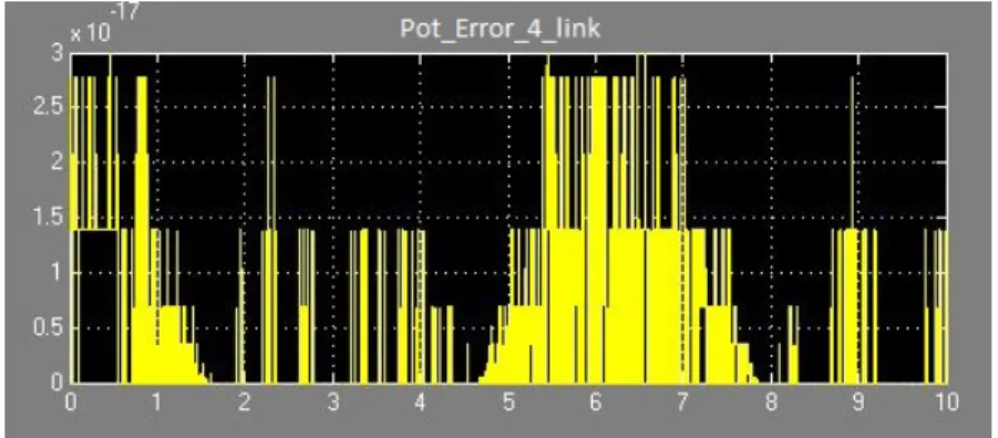
This modeling for the potential of the object has been validated using simulink and the error plot is as follows:

(23)

Figure 8: Error plot for the potential function for object with 4 links

The error is of the order of 10−17 hence validating the potential energy function.

Now, to compute the angles at equilibrium we have to use an equilibrium con-dition which has to be satisfied. At Static Equilibrium, partial differential of the potential energy with respect to the link angles should be zero.

Eqn1 = ∂P

∂θ1

= 0 (8.7)

Eqn2 = ∂P

∂θ2

= 0 (8.8)

Now we have an equation that is solved for given value of xn and yn to obtain

the angle of the first link,θ1 and the second link θ2 at equilibrium at this particular

position for the end point of link 4. This is done usingvpasolve function of MATLAB

which is a numerical solver and gives out the values of θ1 and θ2 which satisfies the

equation in a particular interval. In our case this interval is [0 2π].

Using this value of θ1 and θ2 and substituting in the expressions for θ3 and θ4

we obtain all the equilibrium angles for this pair of xn and yn.

8.3 Equilibrium of 4-link object using Lagrange Multipliers

Using the Lagrange multipliers explained in Section 6.3, we obtain the equations of equilibrium for the 4-link object as:

A=

∂G ∂θ3,4

(8.9)

B=

∂G ∂θ1,2

(24)

τ +BTλ=τa,where, τa=

∂P

∂θ1 ∂P ∂θ2

(8.11)

∂P

∂θ3 ∂P ∂θ4

(8.12)

During equilibrium conditions,τ will be zero. So from the above equations, λ is

solved by taking inverse of BTτa. Multiplying the whole equation by determinant

of BT _{will help avoid problems with finding the solution. After finding} _λ_{, it is}

sub-stituted in 8.12 to get the equations which will be solved for finding the equilibrium angles. The equations along with 8.2 will be used for finding the solution of the four

(25)

9 Obtaining the Configuration Space of the

ob-ject

Now that the modeling of the object is done and a methodology to find equilibrium configuration has been elaborated, this model is used to generate the link angles at equilibrium for all achievable positions for the end-point of the object in Cartesian

space. For a link length of l, the reachable points will be inside a circle of radius

3l. So for each point inside this circle, the corresponding equilibrium link angles are

found and are stored in an array.

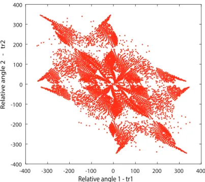
Now to represent each configuration we use the relative angles between two successive links so that the configuration space can be depicted in a two-dimensional image. Hence,

tr1 =θ1−θ2 (9.1)

tr2 =θ2−θ3 (9.2)

wheretr1 and tr2 are the two relative angles for the 3R object.

-400 -300 -200 -100 0 100 200 300 400

Relative angle 1 - tr1

R

ela

tiv

e angle 2 - tr2

Figure 9: Configuration space of the object

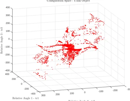
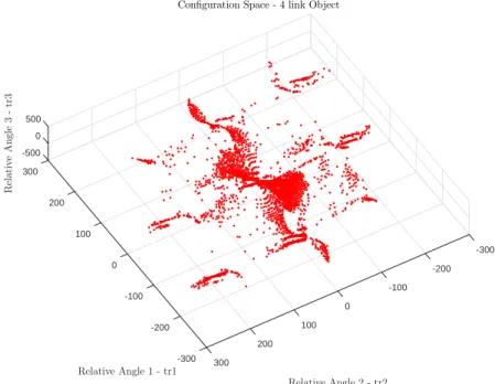
The configuration space for a four-link object will be a 3 dimensional space

(26)

4-dimensional space and so on. As the degrees of freedom increases, it becomes difficult to show graphically the configuration space.

Now to represent each configuration we use the relative angles between successive links so that the configuration space can be depicted in a three-dimensional image. Hence,

tr1 =θ1−θ2 (9.3)

tr2 =θ2−θ3 (9.4)

tr3 =θ3−θ4 (9.5)

(9.6)

wheretr1 , tr2 and tr3 are the three relative angles for the 4R object.

-400 -300 -200

400 -100 0 100 200

R

el

a

ti

v

e

A

n

g

le

3

-tr

3

300 400

200

Relative Angle 1 - tr1 0

Configuration Space - 4 link Object

-200 _-200 -300

Relative Angle 2 - tr2 -100 0

100

-400 ₂₀₀

300

(27)

-400 -200

Relative Angle 2 - tr2 Configuration Space - 4 link Object

0 -400

-300 -200

200 300

-100

200 0

Relative Angle 1 - tr1

R

el

a

ti

v

e

A

n

g

le

3

-tr

3

100 100

200

0 300

-100 400

400

-200 _-300

Figure 11: Configuration space of a 4 link object

-500 300

200

100

-300

0 _-200

-100 -100

Relative Angle 2 - tr2 0 100 -200

200 -300 ₃₀₀ 0

R

el

a

ti

v

e

A

n

g

le

3

-tr

3

500

(28)

10 Configuration Space: Represented as a map

To find a trajectory to move from one configurations of the links to another, we represent the configuration space of the object in the form of a grid map with squares representing each pair of relative angles. The squares marked black have values zero and corresponds to the configurations which are attainable by the object in equilibrium and the squares marked white have a value of 1 and corresponds to the configurations which are not attainable by the object in equilibrium. A part of the big grid map is shown below:

324325326327328329330331332333334335336337338339340341342343 415

416 417 418 419 420 421 422 423 424 425 426 427 428 429 430 431 432 433 434 435

Figure 13: Configuration space represented as a grid map

For a four-link object the same will be a 3D space with black and white cubes. This method is just to help visualize how the algorithm works.

(29)

11 Trajectory Generation

11.1 Objective

The objective of this section is to define a methodology for finding a trajectory to be followed to move from one equilibrium configuration of the object to another one, enabling a dual arm robot to handle the object just like a human could. Now that we have defined a grid map for the configurations, the same could be treated as a path finding problem. The goal will be to move from one square to another in the grid map. Both corresponding to the initial and final configuration. But because all squares are not connected to each other, a small change in the concept of moving between squares will be taken up in the following sections.

11.2 Shortest path Algorithms

Shortest path problems are the ones where one finds a path between two nodes or vertices in a graph which minimizes the sum of the weight of the path followed. The most important algorithms for solving this problem are:

• Dijkstra’s algorithm → solves the single-source shortest path problem. • BellmanFord algorithm →solves the single-source problem if edge weights

may be negative.

• A* search algorithm →solves for single pair shortest path using heuristics to try to speed up the search.

• FloydWarshall algorithm → solves all pairs shortest paths.

• Johnson’s algorithm → solves all pairs shortest paths, and may be faster than FloydWarshall on sparse graphs.

• Viterbi algorithm → solves the shortest stochastic path problem with an additional probabilistic weight on each node.

(30)

11.3 A* (A-Star) Algorithm

A-Star algorithm is a shortest path finding algorithm that finds a locally optimal path when it is possible. Each state is estimated with the following formula that encourages the algorithm to select the state with the closest distance to the goal:

F =G+H (11.1)

where:

• F is the estimated cost of the state

• G is the exact distance from the starting state to the current node

• H is the estimated cost from a given node to the goal

H is the heuristic function that is used to approximate distance from the current location to the goal state. This function is distinct because it is a mere estimation rather than an exact value. The more accurate the heuristic the better the faster the goal state is reach and with much more accuracy.

Algorithm 1 Pseudocode for A* algorithm Put the initial state in the open list

Sb⇐ initial state

repeat

Put the state Sb in the close list (or mark as explored)

for each reachable state Sr from Sb do

if the reachable state is not yet in the list then

Estimate the cost (F=G+H);

Add the reachable state Sr in the open list Mark Sb as the previous state of Sr

else if the new estimation (F=G+H) is better than the previous then

update data in the list

end if end for

Find the best state Sb in the open list

until Sb is the final state

From now on, obstacles will be the squares that represent the unattainable con-figurations of the object. In our case, instead of moving single square by square

(31)

and checking for obstacles, which would lead to no result, as all the squares are not connected with each other, we do the search by considering motions from a square region to another in the grid.

So if there are only obstacles in a given region it is a state that we cannot go to. And if in a region there is atleast one square which is not an obstacle, that region corresponds to a state that we can move to.

In every iteration, the algorithm checks the four square regions that it can move to from the current position and checks if the region is an obstacle and if has already been checked and is in the list. If the region has attainable configurations in it, it chooses the closest to the goal and adds it to the list and marks the current state as the previous state of the reachable state. End the end of the iteration, the best state is found from the list and is chosen as the current state.

The structure of the list is as follows:

X Y G H F Previous Explored(CloseList)

X and Y are the coordinates of the current state, G, H and F are the A* paramenters as explained before. Previous is the position of the previous state in the list as a whole. Explored is either 1 or 0 based on if the state has been explored or not.

5960616263646566676869707172737475767778798081828384858687888990919293949596979899100101102103104105106107108109 381

382 383 384 385 386 387 388 389 390 391 392 393 394 395 396 397 398 399 400 401 402 403 404 405 406 407 408 409 410 411 412 413 414 415 416 417 418 419 420 421 422 423 424 425 426 427 428 429 430

Figure 14: Increments of square areas

Finally when the current state is equal to the goal, the trajectory is found by tracking the path back to the start by using the previous states. The trajectory generated is shown below:

(32)

110112345141312679815161718192021222524232627302829313233353436373839404142434645444748495051525354555659575860616263646566676869707172737475767780797881828384858687889189901001019293959610310294989710510610499107108109110111114112113115116117118119120121122124123125126127128129130131132135134133136137138139140141142143144145146147148149150151152153156155154157158159160161162163164166165167168169170171172173174175176177180179178181182183184185186187188190189191192193194195196197198201200199202203204205206207208209210211214213212215216217218219220221222225223224226227228229230231232235234233236237238239240241242243246245244247248249250251252253254256255257258259260261262263264265266267269268270271272273274275276277280279278281282283284285286287288291290289292293294295296297298301300299302303304305306307308309310311312314313315316317318319320321322325324323326327328329330331332333334335338337336339340341342343344345346349348347350351352353354355356357358359362361360363364365366367368369370371372375374373376377378379380381382383386384385387388389390391392393396395394397398399400401402403404407406405408409410411412413414415416417418419420421422423424425428427426429430431432433434435436438437439440441442443444445446447448449452451450453454457455456458459460461462465464463466467468469470471472473474475478476477479480481482483484485486488487489490491492493494495496499498497502500501503504505506507510509508511512513514515516517518519520523521522524525526527528529530531533532534535536537538539540541544542543547545546548549550551552553554557555556558559560561562563564565568566567569570571572573574575576578577579580581582583584585586589588587591590592593594595596597598599602600601603604605606607608609610611612613614615616617618619620623622621624625626627628629630631634633632635636637638639640641642643644645646647648649650651652655654653656657658659660661662663665664666667668669670671672673674675676678677679680681682683684685686689688687690691692693694695696697700698699701702703704705706707708709710713711712714715716717718719720721722 1 2 3 4 5 6 7 8 9 10 11 12 13 14 15 16 17 18 19 20 21 22 23 24 25 26 27 28 29 30 31 32 33 34 35 36 37 38 39 40 41 42 43 44 45 46 47 48 49 50 51 52 53 54 55 56 57 58 59 60 61 62 63 64 65 66 67 68 69 70 71 72 73 74 75 76 77 78 79 80 81 82 83 84 85 86 87 88 89 90 91 92 93 94 95 96 97 98 99 100 101 102 103 104 105 106 107 108 109 110 111 112 113 114 115 116 117 118 119 120 121 122 123 124 125 126 127 128 129 130 131 132 133 134 135 136 137 138 139 140 141 142 143 144 145 146 147 148 149 150 151 152 153 154 155 156 157 158 159 160 161 162 163 164 165 166 167 168 169 170 171 172 173 174 175 176 177 178 179 180 181 182 183 184 185 186 187 188 189 190 191 192 193 194 195 196 197 198 199 200 201 202 203 204 205 206 207 208 209 210 211 212 213 214 215 216 217 218 219 220 221 222 223 224 225 226 227 228 229 230 231 232 233 234 235 236 237 238 239 240 241 242 243 244 245 246 247 248 249 250 251 252 253 254 255 256 257 258 259 260 261 262 263 264 265 266 267 268 269 270 271 272 273 274 275 276 277 278 279 280 281 282 283 284 285 286 287 288 289 290 291 292 293 294 295 296 297 298 299 300 301 302 303 304 305 306 307 308 309 310 311 312 313 314 315 316 317 318 319 320 321 322 323 324 325 326 327 328 329 330 331 332 333 334 335 336 337 338 339 340 341 342 343 344 345 346 347 348 349 350 351 352 353 354 355 356 357 358 359 360 361 362 363 364 365 366 367 368 369 370 371 372 373 374 375 376 377 378 379 380 381 382 383 384 385 386 387 388 389 390 391 392 393 394 395 396 397 398 399 400 401 402 403 404 405 406 407 408 409 410 411 412 413 414 415 416 417 418 419 420 421 422 423 424 425 426 427 428 429 430 431 432 433 434 435 436 437 438 439 440 441 442 443 444 445 446 447 448 449 450 451 452 453 454 455 456 457 458 459 460 461 462 463 464 465 466 467 468 469 470 471 472 473 474 475 476 477 478 479 480 481 482 483 484 485 486 487 488 489 490 491 492 493 494 495 496 497 498 499 500 501 502 503 504 505 506 507 508 509 510 511 512 513 514 515 516 517 518 519 520 521 522 523 524 525 526 527 528 529 530 531 532 533 534 535 536 537 538 539 540 541 542 543 544 545 546 547 548 549 550 551 552 553 554 555 556 557 558 559 560 561 562 563 564 565 566 567 568 569 570 571 572 573 574 575 576 577 578 579 580 581 582 583 584 585 586 587 588 589 590 591 592 593 594 595 596 597 598 599 600 601 602 603 604 605 606 607 608 609 610 611 612 613 614 615 616 617 618 619 620 621 622 623 624 625 626 627 628 629 630 631 632 633 634 635 636 637 638 639 640 641 642 643 644 645 646 647 648 649 650 651 652 653 654 655 656 657 658 659 660 661 662 663 664 665 666 667 668 669 670 671 672 673 674 675 676 677 678 679 680 681 682 683 684 685 686 687 688 689 690 691 692 693 694 695 696 697 698 699 700 701 702 703 704 705 706 707 708 709 710 711 712 713 714 715 716 717 718 719 720 721 722

Figure 15: Representation of the trajectory

225226227228229230231232233234235236237238239240241242243244245246247248249250 352 353 354 355 356 357 358 359 360 361 362 363 364 365 366 367 368 369 370 371 372 373 374 375 376 377

Figure 16: Representation of the trajectory (Zoomed)

11.4 A-Star applied to higher dimension

(33)

X Y Z G H F Previous Explored(CloseList)

The search will be done in three dimensions. So analogous to the algorithm for the three-link object, we will move in regions but this time not a square, it will be a cube as it is of three dimensions.

To test the algorithm we adopt two points like in Figure 17 as Start and End configurations.

Start = [−60−20−8]

Goal = [9 17 34]

X: -21 Y: -81 Z: -37

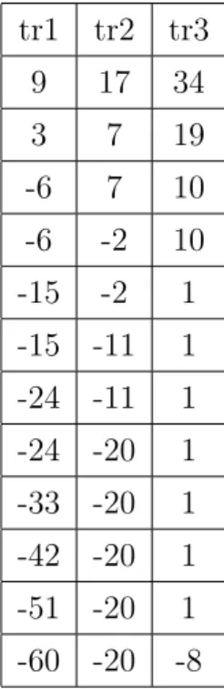
Figure 17: Choosing Start and End Configurations from the Configuration Space The algorithm outputs the trajectory as an array of the configurations through which it has to pass through to reach from the starting configuration to the end configuration.

(34)

tr1 tr2 tr3

9 17 34

3 7 19

-6 7 10

-6 -2 10

-15 -2 1

-15 -11 1

-24 -11 1

-24 -20 1

-33 -20 1

-42 -20 1

-51 -20 1

-60 -20 -8

Table 1: Trajectory in terms of relative angles tr1, tr2 andtr3

The trajectory generated in the configuration space is shown in Figure 18 and 19. This configuration space is for a four-link object under zero gravity angle.

-500 400

200

-300

0 _-200

-100

0 -200

R

el

a

ti

v

e

A

n

g

le

3

-tr

3

100 200 -400

300 500

(35)

Figure 19: Trajectory generated for 4-link object shown in blue

11.5 Probabilistic Road-map Method (PRM)

For configuration spaces of higher degrees of freedom, it is possible to use another method called as Probabilistic Roadmap Method. Probabilistic Roadmap planners

solve motion planning problems where the robot’s configuration space, C is of high

degrees and the environment is defined by thousands of such configurations, defining

the free space F. PRM planner builds only an extremely simplified representation

of F, called a probabilistic roadmap. A roadmap is a graph whose nodes are con-figurations sampled from F according to a suitable probability measure and whose edges are simple collision-free paths, e.g. straight-line segments, between sampled configurations. [9].

In most cases, PRM is used for motion planning algorithms for finding collision free trajectory for a robot. The configuration could be the position of various points on its body and the free space will be the real world with obstacles. In our case, the configuration space is formed the relative angles of the articulated object. So if an

object hasN links, then the configuration space will be of the dimensionN−1. And

we have to find straight line connected paths between two configurations without crossing the obstacles(which in our case are the unreachable configurations) that are there in the configuration space.

PRM planners use two probes based on such algorithms to access geometric

information on the configuration space C:

(36)

Space and C is the configuration space.

• For any pair q, q0 ∈ C, F reeP ath(q, q0) is true if and only if q and q0 can be

connected with a straight-line path lying entirely in F.

The pseudo-code for the algorithm is given below.

Algorithm 2 Pseudocode for a basic PRM algorithm

if F reepath(q1,q2) is truethen

Return path betweenq1 and q2

end if

Initialize the roadmap R with two nodes, q1 and q2.

repeat

Sample a configuration q from C uniformly at random.

if F reeConf(q) is truethen

add q as a new node of R.

end if

for every node v of R such that v 6=q do

if FreePath(q, v) is truethen

add (q, v) as a new edge of R.

end if end for

until q1 and q2 are in the same connected component of R or R contains N + 2 nodes.

if q1 and q2 are in the same connected component of Rthen

return a path between q1 and q2.

else

return NoPath.

(37)

12 Effect of gravity on Object Configuration

To study the effect of gravity on the object configuration, configuration space

cor-responding to different gravity angles P siare studied. It can be seen that the

con-figuration space is not the same and that particular concon-figurations can be attained in certain gravity angles while it cannot be attained in certain others.

-400 -300 -200 -100 0 100 200 300 400

-400 -300 -200 -100 0 100 200 300 400 R el at iv e An gl e 2 -tr 2

Psi = 7pi/10

(a) Configuration Space for a gravity angle of 7π/10

-400 -300 -200 -100 0 100 200 300 400

Psi = 9pi/10

(b) Configuration Space for a gravity angle of 9π/10

-400 -300 -200 -100 0 100 200 300 400

Psi = pi/2

(c) Configuration Space for a gravity angle of π/2

-400 -300 -200 -100 0 100 200 300 400

Psi = -2pi/10

(d) Configuration Space for a gravity angle of -2π/10

Figure 20: Configuration Space for different gravity angles Psi

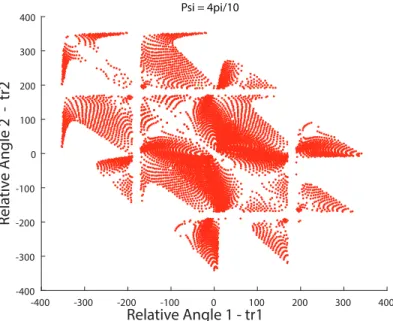
Below is shown the configuration space for two different gravity angles, Psi = 4pi/10 and Psi = 6pi/10.

(38)

-400 -300 -200 -100 0 100 200 300 400 Relative Angle 1 - tr1

-400 -300 -200 -100 0 100 200 300 400

R

ela

tiv

e A

ngle 2 - tr2

Psi = 4pi/10

Figure 21: Configuration Space for a gravity angle of 4π/10

-400 -300 -200 -100 0 100 200 300 400

-400 -300 -200 -100 0 100 200 300

400 Psi = 6pi/10

R

ela

tiv

e A

ngle 2 - tr2

Figure 22: Configuration Space for a gravity angle of 6π/10

Now to understand the effect we zoom in to the same part of the configuration spaces for both gravity angles. It can be seen that, to move from the configuration [-150,320] to [-40,200] is not possible in the case when the gravity angle Psi = 6pi/10 but the same is possible when the gravity angle is 4pi/10. The configuration is given

(39)

my [tr1,tr2] where tr1 and tr2 are the relative angles between the successive links of the object.

-160 -140 -120 -100 -80 -60 -40 -20 0 20

180 200 220 240 260 280 300 320 340 360

Psi = 4pi/10

R

ela

tiv

e A

ngle 2 - tr2

Figure 23: Configuration Space for a gravity angle of 4π/10 (Zoomed)

-180 -160 -140 -120 -100 -80 -60 -40 -20

R

ela

tiv

e A

ngle 2 - tr2

220 240 260 280 300 320 340 360

Psi = 6pi/10

(40)

13 Object manipulation using two 2R-planar robots

13.1 Objective

Now that the modeling, trajectory generation and study of the equilibrium condi-tions under different gravity angles have been completed, we try to implement this manipulation task using two 2R-robots. This will be done by manipulating the two end-points of the object using the two robot end-effectors. This is co-manipulation and even though there are four-DoFs for the two control points of the object, ulti-mately because of two robots manipulating the same object, it becomes 2DoF, i.e; the relative positioning of the two end-effectors.

13.2 Modeling of 2R planar robots

Direct Geometric Model

The direct geometric model for a 2R planar robot is given as follows. L1 and L2

are the length of the proximal and the distal links of the robot. q1 and q2 are the

joint angles and xn and ynare the end-effector coordinates.

xn =L1 ·cos(q1) +L2·cos(q2) (13.1)

yn=L1·sin(q1) +L2·sin(q2) (13.2)

(13.3)

Inverse Kinematic Model

The task space is given by the vector:

X = [xn, yn]T (13.4)

(13.5) The joint space is given by the vector

q = [q1, q2]T (13.6)

The relationship between the joint velocities and the task space velocities is given by

˙

(41)

The jacobian matrix links the joint velocities and the task space.

J =

−L1·sin(q1) −L1·cos(q1)

L1·cos(q1) L2·cos(q2)

(13.8)

13.3 Redundant Manipulation

We have two 2R-robots manipulating two end-points of the articulated object. So we are controlling two degrees of freedom. i.e; the relative position between the two end-points.

We define the manipulation variables as r and t, the horizontal and vertical

distance between the two manipulation points.

r=L1·cos(q12) +L2·cos(q22)−L1·cos(q11)−L2·cos(q21) (13.9)

t =L1·sin(q12) +L2 ·sin(q22)−L1·sin(q11)−L2·sin(q21) (13.10)

Now that we are controlling two degrees of freedom with a four degrees of freedom of the robots, (two degrees of freedom each) we have two degrees of freedom that can be used to achieve more tasks.

(42)

14 Task Priority Approach for Redundant

Ma-nipulators

14.1 Introduction to Task-priority Concept

Robot manipulators are usually designed to have as many number of freedoms as is required by the desired task. But in lots of cases, extra joints are given to make it more dexterous and to add more functionality to the manipulator. They are required to be more flexible and adaptive like a human arm. When the robot end-effector has to follow a specific trajectory, avoiding obstacles, having more degrees of freedom lets it achieve this goal. In [18] a task priority based approach was presented to utilize the extra DoFs of the robot.

This approach deals with the problem of degeneracy, or the situation of not hav-ing enough degrees of freedom to complete all tasks at the same time, by assignhav-ing priorities to the task. So that the task with higher priority is ensured to be executed while the lower priority task is executed as well as possible.

14.2 Inverse Kinematic Solutions with Order of Priority

In this section, the task priority approach [18] is elaborated. We consider the case with two tasks to be executed by the robot. Various papers exists which detail the

(43)

approach with more than two tasks. In our study, as we work with two tasks, we limit the explanation to the task-priority approach for the same.

Considering two sub-tasks defined by the corresponding manipulation variables

T1 ∈ Rm1 and T2 ∈ Rm1 the relationships between the manipulation variable and

the joint-variable q ∈Rn are expressed as follows:

Ti =fi(q) (i= 1,2) (14.1)

(14.2) The differential relationships are given by

˙

Ti =Ji(q) ˙q (i= 1,2) (14.3)

(14.4)

where Ji(q) = ∂fi/∂q ∈ Rmi×n is the Jacobian matrix for the ith manipulation

variable.

The Inverse Kinematic modeling for redundant robots with two tasks is given by:

˙

q =J₁+T˙1+ (In−J1+J1)J2+T˙2 (14.5)

where ˙T1 and ˙T2 are the manipulation variable velocity for the two tasks, In an

identity matrix of size n, in our case n = 4. J₁+ and J₂+ are the pseudo-inverse of

the non-square Jacobian matrices J1 and J2. A pseudo-inverse matrix of a matrix

Am×n _{is defined as a matrix}_A+n×m _{satisfying all of the following four criteria:}

• AA+_A₌_A

• A+_AA+ ₌_A+

• (AA+₎∗ ₌_AA+

• (A+A)∗ =A+A

where A∗ is the Hermitian transpose and AT _{is the transpose of matrix A.}

14.3 Dexterous Manipulation using two 2R planar robots

We have two 2R planar robots with link lengths L1 = 300mm and L2 = 300mm.

(44)

L1

X Y

r

L1 L2

L2

q12 q12 - q22

q11

q11- q21 t

Figure 25: Dexterous manipulation Setup for 3-link object with two 2R planar robots

The joint variable q is defined as the vector of the proximal and the distal joints for both the 2R planar robots.

q = 

  

q11

q21

q12

q22 

  

(14.6)

L1

X Y

r

L1 L2

L2

q12 q12 - q22

q11

q11- q21

t

Figure 26: Dexterous manipulation Setup for 4-link object with two 2R planar robots

(45)

14.4 Definition of First Task

As defined in Section 13.3 we define our first task using the two manipulation variable

r and t

r=L1 ·cos(q12) +L2·cos(q22)−L1·cos(q11)−L2·cos(q21) (14.7)

t=L1·sin(q12) +L2·sin(q22)−L1·sin(q11)−L2·sin(q21) (14.8)

This is the relative positioning of the two end-effectors of the 2R planar robots.

r is the horizontal distance and t is the vertical distance between the end-effectors.

T1 =

r t

(14.9) So now we can define the Jacobian of the first task by partial differential of the function defining the manipulation variables of the first task.

˙

T1 =J1·q˙ (14.10)

J1 =

L1·sin(q11) L2·sin(q12) −L1·sin(q12) −L2·sin(q22)

−L1·cos(q11) −L2·cos(q12) L1·cos(q12) L2·cos(q22)

(14.11) This task ensured the trajectory to be followed for the manipulation of the articulated object. Now to ensure the dexterity of the robot we define a second

task. As the first task takes up only 2 DoF (r and t), we have another 2 DoFs left

for ensuring the dexterity. This will be defined by the relative angle between the two joints of each robot.

14.5 Definition of Second Task

The second task will ensure dexterous manipulation of the object using the two robots. The parameter that defines the dexterity for a 2R planar robot is the angle between its two links. So we can define the second task in the Task-Priority control as follows:

T2 = [q11−q21 , q21−q22]T (14.12)

So now we can define the Jacobian of the second task by partial differential of the function defining the manipulation variables of the second task.

˙

(46)

J2 =

1 −1 0 0

0 0 1 −1

(14.14) Velocity control will be adopted to implement the trajectory following by the pla-nar robots. The velocity command for the manipulation variable will be calculated as

˙

Ti = ˙Ti

0

(t) +Gi·(Ti0(t)−Ti(t)) (14.15)

where ˙Ti is the velocity command for the ith manipulation variable, Ti0(t) is the

desired trajectory, ˙Ti

0

(t) is the derivative of the desired trajectory, and Gi is the

scalar feedback coefficient. The values of Gi are determined experimentally.

For task two, the desired trajectory T0

2(t) can be taken as a constant angle.

T₂0(t) = [pi/2 −pi/2] (14.16)

The joint velocity command is calculated according to the equation 14.17 as follows:

˙

q =J₁+T˙1+ (In−J1+J1)J2+T˙2 (14.17)

14.6 Results and simulation

Below are the results for initial tests run with the proposed task-priority based control law. The plots show the errors for the manipulation variable and the second task variables. It is seen that the first task is well met for a certain period of time and then at the end it shows larger errors. This is due to improper gain tuning.

The gains used are G1 = 3 and G2 = 0.3. Later plots will show a comparison of

different gains and its effect on the performance of the control. However, we can see that the task-priority control law always tries to complete the higher priority task,

i.e; the first task T1 while trying to come closer to the second task as can be seen

(47)

0 1 2 3 4 5 6 7

Time(s)

-20 -10 0 10 20 30 40

E

rr

or

in

r(

t)

Error propagation of First task - r

(a) Error propagation for r

0 1 2 3 4 5 6 7

Time(s)

-40 -20 0 20 40 60

E

rr

or

in

t(

t)

Error propagation of First task - t

(b) Error propagation for t

Figure 27: Error Propagation for First Task T1 -G1 = 3; G2 = 0.3

0 1 2 3 4 5 6 7

Time(s)

-20 -10 0 10 20

E

rr

or

in

q

11-q

21(

t)

Error propagation of Second task

(a) Error propagation forq11−q21

0 1 2 3 4 5 6 7

Time(s)

-10 -5 0 5 10

E

rr

or

in

q

12

-q

22(

t)

(b) Error propagation forq12−q22

Figure 28: Error Propagation for Second Task T2- G1 = 3; G2 = 0.3

14.7 Gain Tuning for the two Tasks

We take up the study of the effect of changing gains G1 and G2 on the performance

of the system. We will be testing a trajectory that has been generated using the previously elaborated methods. The goal is to manipulate the object from an initial configuration of [-150,320] to a final configuration of [-40,200], where the values rep-resent the relative angles between the links of the object. The trajectory is obtained first in terms of the x and y coordinates of both the robot end-effectors. Then this is transformed to the r and t coordinates representing the relative positioning of the end-effectors. We have a spline array of values for r and t, which we input to the task-priority control algorithm and also differentiate to find the manipulation variable velocity.

(48)

14.7.1 Tuning the gain G1

First we keep G2 constant and change G1. We take four values of G1

G1 = 

  

0.5 1 2 5     (14.18)

G2 = 0.3 (14.19)

The initial configuration of the robot is:

q=     π/2 0 π/2 3π/2



  

This leads to an initial T1 as

T1stby =

100

0

(14.20)

The results for the different values of G1 are shown below. In Fig 28 the errors of

the task 1 T1 implementation is shown when G1 is changed while keeping G2 at a

constant value of 0.3. As can be seen the gain in the range of 0.5 - 1 gives good performance and is stable till the end of the task execution. Higher values of gain

G1 shows unfavorable behavior by the end of the simulation.

0 1 2 3 4 5 6

Time(s) -40 -30 -20 -10 0 10 20 30 40 E rr or in r( t)

Error propagation of First task - r G1 = 0.5 G1 = 1 G1 = 2 G1 = 5

(a) Error propagation forr

0 1 2 3 4 5 6

Time(s) -40 -30 -20 -10 0 10 20 30 40 E rr or in t( t)

Error propagation of First task - t G1 = 0.5 G1 = 1 G1 = 2 G1 = 5

(b) Error propagation fort

Figure 29: Error Propagation for first task T1 when gain G1 is changed

Fig 34 shows the error plot for the evolution of the first task T1 when G1 is

changed while keeping G2 at a constant value of 0.3. The plots show similar

(49)

behavior of the error in the case of task 2 is such that the control law tries to bring it closer to the reference values as much as possible.

0 1 2 3 4 5 6 7

Time(s) -20

-10 0 10 20 30 40

E

rr

or

in

q

11-q

21(

t)

Error propagation of Second task G1 = 0.5

G1 = 1 G1 = 2 G1 = 5

0 1 2 3 4 5 6 7

Time(s) -10

-5 0 5 10 15 20 25

E

rr

or

in

q

12

-q

22(

t)

G1 = 1 G1 = 2 G1 = 5

Figure 30: Error Propagation for Second task T2 when gain G1 is changed

14.7.2 Tuning the gain G2

Fig 35 shows the error for the first task when G2 is changed and G1 is kept at a

constant value.

G2 = 

    

0.0 0.1 0.3 0.5 0.8 

    

(14.21)

G1 = 1 (14.22)

As can be seen from 35 change in the gain G2 has very little effect on the execution

of task 1. it almost remains the same. But from the plot for the evolution of task 2

from the figure 36 we can see that as G2 is increased there is considerable decrease

(50)

0 1 2 3 4 5 6 Time(s) -40 -30 -20 -10 0 10 20 30 40 E rr or in r( t)

G2 = 0.0 G2 = 0.1 G2 = 0.3 G2 = 0.5 G2 = 0.8

0 1 2 3 4 5 6

Time(s) -40 -30 -20 -10 0 10 20 30 40 E rr or in t( t)

G2 = 0.0 G2 = 0.1 G2 = 0.3 G2 = 0.5 G2 = 0.8

0 1 2 3 4 5 6 7

Time(s) -20 -10 0 10 20 30 40 E rr or in q 11-q 21( t)

G2 = 0.1 G2 = 0.3 G2 = 0.5 G2 = 0.8

0 1 2 3 4 5 6 7

Time(s) -10 -5 0 5 10 15 20 25 E rr or in q 12 -q 22( t)

G2 = 0.1 G2 = 0.3 G2 = 0.5 G2 = 0.8

14.8 Effect of standby position of robots on the control

We try the same with another stand-by position for the robot and the results are shown below:

The initial cofiguration of the robot is:

q=     π/2 π/4 π/2 3π/4



  

This leads to an initial T1 as

T1stby =

275.7359

0

(51)

0 1 2 3 4 5 6 Time(s) -40 -30 -20 -10 0 10 20 30 40 E rr or in r( t)

G1 = 0.5 G1 = 1 G1 = 2 G1 = 3 G1 = 5

0 1 2 3 4 5 6

Time(s) -40 -30 -20 -10 0 10 20 30 40 E rr or in t( t)

G1 = 0.5 G1 = 1 G1 = 2 G1 = 3 G1 = 5

0 1 2 3 4 5 6 7

Time(s) -20 -10 0 10 20 30 40 E rr or in q 11-q 21( t)

G1 = 0.5 G1 = 1 G1 = 2 G1 = 3 G1 = 5

0 1 2 3 4 5 6 7

Time(s) -80 -60 -40 -20 0 20 40 E rr or in q 12 -q 22( t)

G1 = 0.5 G1 = 1 G1 = 2 G1 = 3 G1 = 5

0 1 2 3 4 5 6

Time(s) -40 -30 -20 -10 0 10 20 30 40 E rr or in r( t)

G2 = 0.0 G2 = 0.1 G2 = 0.3 G2 = 0.5 G2 = 0.8

0 1 2 3 4 5 6

Time(s) -40 -30 -20 -10 0 10 20 30 40 E rr or in t( t)

G2 = 0.0 G2 = 0.1 G2 = 0.3 G2 = 0.5 G2 = 0.8

(52)

0 1 2 3 4 5 6 7 Time(s) -20 0 20 40 60 80 E rr or in q 11-q 21( t)

G2 = 0.1 G2 = 0.3 G2 = 0.5 G2 = 0.8

0 1 2 3 4 5 6 7

Time(s) -80 -60 -40 -20 0 20 E rr or in q 12 -q 22( t)

G2 = 0.1 G2 = 0.3 G2 = 0.5 G2 = 0.8

14.9 Adaptive Gain Change for obtaining minimum error

As is observed from figures 29, the performance changes with respect to time and the values in the spline. This can be overcome by an adaptive gain which changes

according to the error evolution. G1 can change values to obtain the minimum error

possible for executing the task T1. The results with adaptive gain is plotted below.

We can clearly see the better error results for taskT1 in Fig.37 and the gain changes

has also been shown in 38

0 1 2 3 4 5 6

Time(s) -40 -30 -20 -10 0 10 20 30 40 E rr or in r( t)

0 1 2 3 4 5 6

Time(s) -40 -30 -20 -10 0 10 20 30 40 E rr or in t( t)

Definition of an active deformation model for manipulation of flexible objects

Master ARIA - ROBA

Thesis Report