Comparing the structure of power-law graphs and
the Internet AS graph
Sharad Jaiswal, Arnold L. Rosenberg, Don Towsley
Computer Science DepartmentUniv. of Massachusetts, Amherst
{sharad,rsnbrg,towsley}@cs.umass.edu
Abstract— In this work we devise algorithmic techniques to compare the interconnection structure of the Internet AS Graph with that of graphs produced by topology generators that match the power-law degree distribution of the AS graph. We are guided by the existing notion that nodes in the AS graph can be placed in tiers with the resulting graph having an hierarchical structure. Our techniques are based on identifying graph nodes at each tier, decomposing the graph by removing such nodes and their incident edges, and thus explicitly revealing the interconnection structure of the graph. We define quantitative metrics to analyze and com-pare the decomposition of synthetic power-law graphs with the Internet-AS graph. Through experiments, we observe qualitative similarities in the decomposition structure of the different fami-lies of power-law graphs and explain any quantitative differences based on their generative models. We believe our approach pro-vides insight into the interconnection structure of the AS graph and will find continuing applications in evaluating the representa-tiveness of synthetic topology generators.
Index Terms—Internet Topology, AS Graph, power-law graphs
I. INTRODUCTION
In recent years, a significant amount of work has focused on understanding the properties of the Internet Autonomous Sys-tem graph. In their pioneering study which compared
graph-based models for the Internet topology, Zeguraet al.[24]
iden-tified that the Internet has anon-random structurethat was not
captured by then-existing topology generators. Specifically,
they emphasized the presence of anhierarchy in the manner
in whichAutonomous Systems1 were interconnected.
Subse-quently, another important set of observations was reported by
Faloutsoset al.[10], regarding the statistical properties of some
metrics of the Internet graph. Using measurements of the con-nectivity of the Internet nodes at both the router and the AS level, they found that several graph metrics such as the distri-butions of node degrees, the degree ranks of the nodes, and
the number of nodes within hhops of each other, could be
described by power-laws. The presence of power-laws in the Internet graph is now considered to be empirically well estab-lished. Similarly the notion of an hierarchical structure in the Internet graph, and the presence of a routing hierarchy has also been commonly noted in literature [24], [13]. These observa-tions have been a starting point for a flurry of work on devel-oping synthetic Internet topology generators. Generators such
1An AS is a group of routers and end-hosts that have common routing
poli-cies, with respect to the rest of the Internet.
as Tiers andTransit-Stubcreate graphs with an explicit hier-archical structure as a model for the Internet. From another
starting point, work by Barabasiet al.[5], Aielloet al.[2] and
others [7], [17], [15] has led to topology generators that aim primarily to match the power-law degree distribution of the In-ternet graph.
There have been several studies comparing power-law de-gree based generators and the Internet graph. In [18], the au-thors compared the graphs produced by these generators based on metrics such as power-law exponents, degree rank,
hop-plot and eigenvalue distributions. In [7] the authors
intro-duced the clustering coefficient and the median shortest path length as useful metrics for distinguishing among the different
topology generators. And, most recently, Tangmunarunkit et
al.[22], carried out an extensive comparison study, using a wide
range of metrics, including expansion (neighborhood size), re-silience (size of a cut-set for a balanced bipartition) and distor-tion (minimum-communicadistor-tion-cost spanning tree). Although there isn’t yet a consensus on which of the above-mentioned metrics are the most important, one common property of these metrics is that they do not give insight into the structure of the graph. Our work in this paper addresses the following
ques-tion: how well do power-law graphs capture theinterconnection
structure(such as hierarchy) of the Internet graph?
One possible way of thinking about the “structure” of a graph is by comparison with canonical topologies such as a star, a mesh or a binary tree. In our context, there is a widespread belief that the Internet graph is hierarchical in structure. In this study, we use algorithmic techniques to explore the struc-tural properties of power-law graphs with respect to the Internet graph, guided by existing notions of how ASes connect to each other. Using the notion that ASes are arranged in tiers, we iden-tify nodes at each tier, and recursively decompose the graph to expose its interconnection structure. We define metrics of the resulting decomposition, which then allow us to quantitatively and statistically compare the structural properties of power-law graphs and the Internet graph. The properties of the decompo-sitions of these graphs allow us to also examine questions like whether the graph is hierarchical in nature. We observe, and through statistical tests exhibit, similarities in the decomposi-tion structure of power-law graphs as compared to the Internet AS graph. We also find that both the skewed-degree distribu-tion and the degree of preferential connectivity play a role in defining the decomposition structure of these graphs. These
two properties cause a large number of nodes (which also have small-degrees) to directly depend on the high-degree nodes for connectivity to the rest of the graph, and also contribute to the resiliency of the graph by causing high-degree nodes to connect with each other.
The rest of this paper is organized as follows. In Section II, we elaborate on existing notions of the structure of the
In-ternet graph. Section III introduces algorithmic techniques
which leverage knowledge of structural properties of the ternet graph and apply them to power-law graphs and the In-ternet graph, to achieve an hierarchical decomposition of these graphs. We describe some metrics of interest which can be used to compare the decompositions of the different graphs. We also describe some related work which has also examined issues like the presence of an hierarchy in the AS graph, and in power-law random graphs. In Section IV we introduce the graph families that we examine as part of this study. Section V discusses the results from the decomposition, and their implications for the structure of the graphs. We also examine the decompositions of the different families of graphs, and compare the similari-ties in more detail through statistical tests. We describe future directions for this work, and conclude in Section VI.
II. STRUCTURE OF THEASGRAPH
The Internet is composed of a collection of administrative
domains calledAutonomous Systems. Based on the properties
of the routes starting, ending or passing through an AS, it can be
classified as either astubor atransitAS. As defined in [24], a
stub AS is one such that the path connecting any two end-hosts,
u andv, in the Internet traverses this AS only if eitheruor v
belongs to this AS. Transit ASes do not have this restriction, and can hence serve as an intermediary in any path. Stub ASes usually correspond to universities or large commercial organi-zations, which rely on transit ASes for connectivity to the rest of the Internet. They themselves do not offer such a service to any
other AS. Transit ASes, in Internet terms, areservice providers
and are typically regional and national level ISPs, orbackbone
networks. They offer connectivity to several stub ASes and are also well-connected to each other.
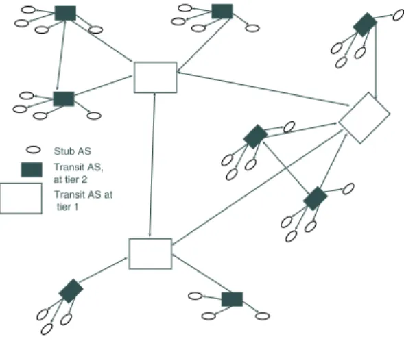
Stub AS Transit AS, at tier 2 Transit AS at tier 1
Fig. 1. Structure of the AS graph
The notions of transit and stub domains suggest a structure as to how ASes connect in the Internet. Stub nodes connect with
one or more transit nodes, and all paths originating or
culminat-ing in a Stub node must traverse theseprovidertransit nodes.
Also, transit domains can be either providers to, orcustomers
of other transit nodes. Thus, based on these provider-customer relationships, each AS in the Internet can be considered as
be-longing to a particular tier2, with the ASes at the highest tier
being the transit domains that have no providers (the so called Tier-1 providers). Stub ASes are completely dependent on the transit nodes in the tier above for connectivity to the rest of the Internet (to a lesser extent, this is true also of lower tier transit ASes. However transit ASes can also route some traffic through
peeringrelationships they have with other transit ASes in the same tier.).
The arrangement of nodes into different tiers, as described above, and the relationship between the transit and stub ASes also provides a possible hierarchical structure of the Internet graph. One can conceive of the Internet as composed of a set of transit ASes at the top of the hierarchy, offering connectiv-ity to both transit and stub ASes, at the next tier. The second tier transit ASes themselves provide connectivity to other ASes below them, and so on. In Section III, we introduce techniques that allow us to examine the structure of the graph based on this notion.
III. EXPLORING STRUCTURE
We now describe the technique we use to understand and compare the structure of the Internet AS graph with those of graphs that have been generated to simply match the power-law degree distribution of the AS graph. Our efforts are guided by the interconnection properties of the transit and stub nodes in the Internet AS graph, as described in the previous section.
We begin by describing a criterion to identify the root-level transit nodes. We then decompose the graph by removing these nodes and their incident edges from the graph. The procedure is then repeated recursively, over every connected component of the resulting graph. A concise description of the procedure is as follows:
1) Given an input graph,G, select a set of nodes to be
re-moved.
2) Compute the connected components (CCs) of the graph
Gobtained after removing the selected nodes.
3) Repeat the procedure recursively on the resulting CCs, until the number of nodes that can be removed is less than
1.
This technique serves two objectives. It assigns the nodes of the graph to a particular level (or tier): at each level of decom-position, the nodes selected for removal belong to that level. Also, the decomposition of the graph at each level exposes the interconnection structure among nodes within that level.
A key aspect of this technique is the criterion used to select nodes to be removed at each level of the decomposition. Our
first choice for this metric is based onnode degree. We order
the nodes in each connected component in descending order
of degree and choose a fixed fractionαof the highest degree
nodes to remove. We justify using this metric by looking into the degree of the ASes in the Internet in relation to the tier to
2or “level”; we use the terms “level” and “tier” (to which a node belongs)
Average degree Tier 1 614.29 Tier 2 19.30 Tier 3 6.93 Tier 4 4.30 TABLE I
AVERAGE DEGREE OFASES IN DIFFERENT TIERS
which they belong. Using the inference techniques developed in [12], we first arrange the ASes into their respective tiers. The
average degrees of theProviderASes3 appears in Table I. As
can be observed, the average degree of the ASes decreases as we go down the tiers, suggesting a positive correlation between a node’s tier and its degree. In Figure 2 we plot the ASes, ar-ranged in the x-axis as per the tier to which they belong, with their respective degrees in the y-axis. Looking at this figure we observe that in the actual Internet, an AS with a smaller degree can be placed at a tier higher than an AS with a higher degree. This indicates that node degree does not completely capture the semantics of how ASes are placed in the real AS graph.
0 0.5 1 1.5 2 2.5 3 3.5 0 0.5 1 1.5 2 2.5 3 3.5 Log10(As Index) log10(Node Value) Tier1 Tier2 Tier3 Tier4
Fig. 2. Degree of ASes in different tiers
We considered two other metrics. The first isnode rank, a
notion adapted fromPageRank, a metric developed in [19] to
rank web pages. (A similar notion to capture the “authority” of web pages was also developed in [16].) Let the nodes of the graph be denoted1,2, ..., N. Letd(j)denote the degree of node
j, and letN b(j)denote the set ofj’s neighbors in the graph.
Thenr(j)is the steady-state probability of visiting nodejwhile performing a random walk in the graph where each outgoing
link from a node is equally likely to be chosen,r(j)satisfies
r(j) =
i∈Nb(j)
r(i)
d(i)
3The provider ASes correspond to the nodes we seek to remove at each level
of decomposition.
N
j=1
r(j) = 1
This metric is computed iteratively. Initially all nodes are
assigned the rank-value 1/N. At each step, the ranks of the
nodes are computed based on the above definition and normal-ized such that ranks of all nodes sum to 1. This procedure is
repeated until the values of the node ranks converge4. Our third
choice of the metric isnode stress, a metric that is based on the
link valuemetric defined in [22]. Thestressof a nodev in a graph, is a measure of the number of node-pair shortest paths
that pass throughv. We define thenode stressof any node in the
graph to be the size of its traversal set, normalized by the num-ber of all node-pairs in the graph. The traversal set of a node
v is the set of all node-pairs(s, d)in the graph, whose
short-est path traverses nodev. After computing theNode Stressand
Node Rankof all nodes in the input graphs, we found that there is a very strong correlation between the degree of the node and itsstressor rank. Therefore, we do not obtain any new infor-mation about the interconnection semantics of the input graphs using these metrics. Hence we restrict ourselves to presenting results of the decomposition procedure, using only the node de-gree metric.
We describe some metrics that allow us to characterize a de-composition quantitatively.
• NCC quantifies the number of CCs at any level of the
decomposition.
• σCC is the standard deviation of the sizes of the CCs at
each level.
• Dthe depth of the decomposition, i.e., number of levels of
recursion until we do not find any more nodes to remove from the CCs at that level of recursion.
• We also examine the distribution of sizes of the CCs at
each level of decomposition, and the distribution of node degrees in the largest CC at each level of decomposition. In addition to exposing the interconnection structure of the input graph, this decomposition procedure allows us to examine whether the graph has hierarchical properties. Although there is no precise general notion of hierarchy, one way of think-ing about it is in terms of classical hierarchical graphs, such as rooted trees. A key characteristic of such graphs is that a
path from a node vin this graph, to any other node (which is
not a descendant ofv) passes through the parent ofv. Hence the
removal of nodes belonging to a higher tier would partition the graph of the remaining nodes at tiers below. One can observe an appropriate parallel of this characteristic in the Internet graph. The transit nodes with no providers would form the “root” tier, and other transit and stub nodes would successively be arranged in the tiers below, based on the relationships among these ASes. However, it is not clear if this structure is hierarchical in the sense of the rooted trees, described above. It is worth noting that breaking a graph into tiers does not necessarily shed any light into whether it has an hierarchical structure, since tiering does not impose the notion that nodes in a tier depend on the
4Another way of computing the Node Rank is to consider the stochastic
ma-trix derived from normalizing the columns of the adjacency mama-trix of the graph under consideration. The Node Ranks of the graph nodes are then the values in the principle eigenvector of the stochastic matrix [19].
one above them for connectivity. Nodes within a tier could be well connected within themselves, and perhaps also to nodes in tiers above the one immediately on top of them. In fact, a tiering could be induced in any graph, hierarchical or not. We soon discuss this in more detail, and explore to what extent the graphs we examine exhibit such hierarchical characteristics.
A. Related studies
There has been some previous work incharacterizingthe
hi-erarchy of the Internet graph. In [13], the authors observed that ASes can be divided into four classes, with significant variation of average degree between the classes. The authors propose a tiering induced upon the AS graph, with the class of ASes with the highest average degree at the top tier, followed by others in descending order of the average degree. A similar tiering of ASes has also been introduced in [12], [21], but using the logi-cal relationships between the ASes. In [12], the authors create a logical tiering based on the Customer-Provider relationship between ASes, with a Provider AS assigned a tier higher than its Customer. A similar approach has been suggested by [21], using logical relationships and some notion of node intercon-nectivity to distinguish adjacent tiers. A recent work [22] also considers the hierarchical characteristic of the Internet graph, and the degree to which the degree based generators capture
this property. Their metric of choice is the distribution of
link-values, where the value of a link can be roughly defined as the number of node pairs whose shortest paths traverse this link. The authors study the distribution of link-values for the Inter-net router and AS level graphs, power-law graphs and some canonical graphs. Examining the distribution of this metric for different topologies and comparing it with the distribution of the classical tree topology, the authors qualitatively compare the relative degrees of hierarchy of graphs of different topolo-gies. Although this metric serves a useful purpose in distin-guishing among the different graphs, it falls short of answering several questions. The distribution of link-values does not lend any insight into the interconnection structure of the graph which would have led to this distribution. Also, observing the distri-bution of link-values does not answer some questions about the nature of the hierarchy, whether it is balanced, how deep is it etc. In other words, we are not able to “visualize” the structural properties of these graphs.
IV. INPUT GRAPHS
We now introduce the set of graphs that we examine. The Autonomous Systems topology has been created from
the BGP routing tables collected at the route-views server
(route-views.oregon-ix.net). The route-viewsdata
set consists of routing tables exported from BGP routers of var-ious Tier-1 ASes, and provides one of the most comprehensive views of the current Internet. Since BGP is a path vector proto-col, the routes advertised in these tables can be used to infer AS adjacencies and thus the AS graph. One problem with this ap-proach is that ASes selectively announce routes to other ASes based on the contractual agreements between them. Hence, if we have information only from some select BGP routers, we may miss out on some advertised routes (and hence AS adja-cencies) in the AS graph. In a recent work [8] the authors have
discussed this problem, and have extended theroute-viewsdata
set with BGP routing tables of a few other ISPs, and entries from the Internet Routing Registry. They found the AS topol-ogy constructed from this data set to have a significant number of extra edges. Moreover, the degree distribution of this aug-mented AS graph was found to not conform to a strict power-law distribution. The authors also examined the nature of these missing edges between the the two data sets, and found that most were either peer-peer edges between lower-tier ASes, or customer-provider edges. We applied our decomposition
tech-niques on AS graphs constructed from both theroute-viewsand
the extended data set. We found (as will be discussed in detail in Appendix A) that our results and observations hold across these two different topologies. Moreover, a major source of the extra edges in the extended topology (nearly 72% [8]) are customer-provider links. These are from a multi-homed AS to its providers, and may be fail-over links that are used only when the primary link is not operational. This brings into question the relevance of some of the missing edges between the two data
sets. Based on these points, we chose to adopt theroute-views
data set as our AS topology of reference for this study. Finally, even though the degree distribution of the AS graph constructed
from theroute-viewsdata set may not follow a strict power-law,
these graphs share important characteristics. Both have a highly skewed degree distribution, and common generative principles such as a notion of preferential connectivity. These character-istics, as we will soon observe, play a key role in determining the decomposition structure of these graphs. Thus, we argue, power-law graphs are relevant models for comparison with the AS graph.
We represent the AS level topology of the Internet by a graph,
G =< V, E >, where eachv ∈ V denotes an AS and each
e ∈ Eis an undirected inter-AS connection inferred from the
routing table data. We use the routing tables from May, 2004 to construct the AS topology. Next, we consider two variants of power-law based degree generators,
• PLRG(power law random graph) is a generator developed
in [2]. Given a target number of nodesNand a power-law
exponentβ, PLRG first assigns degrees to all the nodes
drawn from this power-law distribution. It then randomly matches degrees among all the nodes. This procedure may produce graphs which are not connected, as well as graphs that have have self-loops and duplicate links. It has been shown in [2] that there exists a giant connected
compo-nent, for a large range of values ofβ. We hence search for
this giant connected component and remove all duplicate links and self-loops.
• GLP(generalized linear preference) [7] extends the
tech-nique proposed in [5]. Starting with a small set of core nodes, the technique incrementally constructs the graph. At each step, one of two operations is probabilistically
chosen(i)adding a new node along withm links, or(ii)
addingmnew links without a node. In both cases, the links
are connected to existing nodes with a probability that is proportional to their degrees.
As a means of comparison with classical random graphs,
we also choose topologies generated by theWaxman
genera-tor [23]. The classical Erdos-Renyi random graph model [6] assigns a uniform probability for creating a link between any
AS Graph PLRG GLP Waxman
Number of Nodes 17611 17525 17611 17611
Number of Edges 38015 43377 27199 35222
TABLE II
CHARACTERISTICS OF THEINPUT GRAPHS
AS Graph PLRG GLP Waxman
Depth 9 14 6 37
TABLE III
DEPTH OF THE DECOMPOSITION
pair of nodes. The Waxman generator extends the classical model by randomly assigning nodes to locations on a plane and making the link creation probability a function of the Euclidean distance between the nodes.
Table VII describes some specific properties of the studied graphs. We use the Autonomous System graph inferred from the Route-view server’s routing table data collected on May, 2004, as our reference graph. The topologies generated us-ing other generative mechanisms aim to match the AS graph in terms of numbers of nodes and edges. We generated 100 instances of these graphs with a different initial seed for each instance; the table presents the average quantities computed over all these instances. The empirical complementary cumu-lative distribution of the node degrees of the AS graph follows
a power-law, with an exponentβ =−1.125. The graphs
gen-erated by the PLRG and GLP generators closely (although, not exactly) match this exponent.
V. RESULTS FROM THE DECOMPOSITION
Initially we choose a fixed value ofα= 0.01 5the fraction of
nodes to be removed from the CCs of the graph at each level of
decomposition. We later use different values ofα, at different
levels of decomposition and briefly discuss the differences in results in Appendix C.
Let us first consider the decomposition of the graphs with power-law degree distributions, namely the AS graph, PLRG and GLP graphs. We start by removing the top 1% highest degree nodes and their edges from the input graph. We then identify the CCs in these decomposed graphs, and repeat the
5Studies have reported that about 1% of all ASes in the Internet have no
providers. About 20 of these ASes have been found to form (almost) a clique, which would be another (lower) estimate of the Tier-1 ASes.
AS Graph PLRG GLP Waxman Level 1 8267 7651 11414 7 Level 2 1190 697 380 18 Level 3 749 492 238 23 Level 4 375 392 145 32 Level 5 273 326 73 39 TABLE IV
NUMBER OFCCS AT THE FIRST FIVE LEVELS OF THE DECOMPOSITION
0 2 4 0.75 0.8 0.85 0.9 0.95 1
x: log10(size of the connected component)
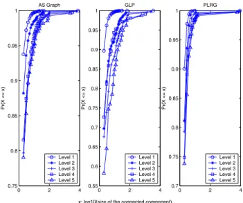
Pr(X <= x) AS Graph Level 1 Level 2 Level 3 Level 4 Level 5 0 2 4 0.55 0.6 0.65 0.7 0.75 0.8 0.85 0.9 0.95 1 Pr(X <= x) GLP Level 1 Level 2 Level 3 Level 4 Level 5 0 2 4 0.7 0.75 0.8 0.85 0.9 0.95 1 Pr(X <= x) PLRG Level 1 Level 2 Level 3 Level 4 Level 5
Fig. 3. CDF of the sizes of CCs of first 5 levels of decomposition
AS Graph PLRG GLP Waxman Level 1 45% 50% 21% 99% Level 2 76% 88% 73% 99% Level 3 66% 90% 66% 99% Level 4 80% 90% 54% 99% Level 5 75% 90% 51% 99% TABLE V
PERCENTAGE OF NODES IN THE LARGESTCCIN THE FIRST 5LEVELS OF DECOMPOSITION
procedure recursively. In all three classes of graphs, we observe nontrivialsized CCs until a level of recursion ranging from 6 -14 as shown in Table III.
One observes in Table IV that the removal of the selected nodes decomposes the graph into a large number of CCs. The distribution of the sizes of these CCs is, however, highly skewed, with a large fraction of CCs being trivial. This can also be observed in Figure 3, which plots the CDF of this distribu-tion, and indicates that between 80-90% of all CCs have either 1 or 2 nodes. Although we have not yet carried out statistical tests to back this claim, visually these distributions seem similar, for the AS, PLRG and GLP graphs. The disparity in the sizes of the
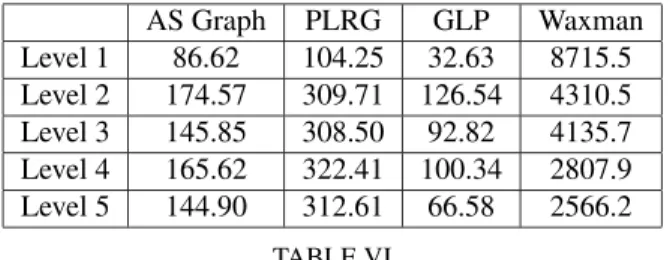
CCs is also reflected in Table VI which computesσCC, which
are extremely high across the three families of graphs. The next common characteristic of the decomposition is the existence of a “giant” CC at each level of decomposition. This giant CC, as shown in Table V, contains 21-50% of nodes in the first level, and 50-90% of nodes in subsequent levels. However, there is also a substantial difference in the relative sizes of the giant CC in the first level of decompositions of GLP graphs (21%), AS Graphs (45%) and PLRG Graphs (50%). We consider the rea-sons behind this difference imminently.
The decomposition structure of the power-law graphs is strik-ingly different from that of the Waxman graph. Removing the highest-degree nodes from that graph fails to decompose the graph in any significant measure. As can be seen from Table IV, a very small number of CCs are formed at each level of the
de-AS Graph PLRG GLP Waxman Level 1 86.62 104.25 32.63 8715.5 Level 2 174.57 309.71 126.54 4310.5 Level 3 145.85 308.50 92.82 4135.7 Level 4 165.62 322.41 100.34 2807.9 Level 5 144.90 312.61 66.58 2566.2 TABLE VI
STANDARD DEVIATION OF THESIZE OFCCS IN THE FIRST 5LEVELS OF THE DECOMPOSITION
composition, with one CC comprising almost all nodes of the graph, and a few trivially sized CCs. This is not surprising since in a classical Erdos-Renyi random graph, most nodes have a de-gree close to the mean dede-gree of the graph, with the maximum degree of the graph being orders of magnitude smaller than the maximum degrees in a similar sized power-law graph. Hence, the removal of the highest degree nodes has a very limited im-pact on the structure of the graph. This difference also trans-lates into a significantly larger depth of decomposition for the Waxman graph. PLRG GLP 35 40 45 50 55 60
% of nodes with degree <=10 connected to highest 1\% degree nodes
AS Graph = 46%
Fig. 4. A measure of the preferential connectivity in PLRG, GLP and AS
Graphs
We now explain why there is a significant difference in the relative sizes of the giant CCs, in the first level of decomposi-tion among the three graph families. We know that these graphs have a very skewed degree distribution (80% - 90% of nodes
in the three graph families have degree≤3, and 95% of node
have degrees≤10) and the node-degrees of the highest-degrees
nodes are orders-of-magnitude higher than the average node de-gree. We observe also that most nodes that are not in the gi-ant CC belong to trivial sized connected CCs. One explanation for this could be that nodes with small degrees comprise most of the neighbors of nodes with the largest degrees. Removing the highest-degree nodes could disconnect many of these low-degree nodes, which would then form trivial-sized connected CCs. In order to understand how this observation helps explain the difference in the relative sizes of the giant CCs, we examine Figure 4 which is a box-plot of the percentage of nodes with
degree≤ 10, that are connected only to the removed
highest-degree nodes. We notice that GLP graphs have, in general, a much higher fraction of small-degree nodes connected solely to the highest degree nodes (median: 60%), as compared to the AS Graph (median: 46%), which in turn has a higher percent-age of such nodes than PLRG graphs (median: 41%). Removal of the highest degree nodes in the GLP graphs thus disconnects a greater percentage of nodes in the remaining graph, as com-pared to PLRG and AS Graph. This directly leads to a smaller size of the giant CC in the GLP graphs. On the other hand, PLRG graphs, which have the smallest percentage of small-degree nodes connected to the highest-small-degree nodes, have larger giant CCs resulting from the decomposition. This difference in structure can be explained by the differences in the connectivity models of these graphs. PLRG graphs are based on a linear-preference connectivity model, while it has been reported in [9] that in the Internet, new ASes have a much stronger preference to connect to large-degree ASes than predicted by the linear preference model. GLP graphs have been designed explicitly to incorporate this greater than linear preference for new ASes, in order to connect with ASes with large degrees.
To further support our observation that connection prefer-ences of lower-degree nodes determine the sizes of the gi-ant CCs, we have also constructed power-law graphs with a preference for high-degree nodes, to connect with the lowest-degree nodes (as described in Appendix B). Since nearly all the smallest-degree nodes in such graphs are connected to the highest-degree nodes, the decomposition results in no giant
CCs at any level of decomposition.6
We now address the question of whether these graphs are hi-erarchical. First, the graphs’ decompositions tend to be highly imbalanced, with the size of the largest CC being orders of mag-nitude larger than the average size of the CCs. Second, there are many CCs at each level of the decomposition. Referring to our previous discussion, a criterion we stipulated for a graph to be hierarchical was that nodes (aside from those in the topmost level) would depend on the nodes in the level above for paths to the rest of the graph. This is true for the decomposition of the graphs we have studied, since members of the (numerous) small CCs are disconnected from the graph upon removal of the nodes at a higher level. Also, these nodes form a substan-tial fraction of nodes (50% to 79% at decomposition level 1). Thus, based on this criterion, the resulting decomposition does have hierarchical properties. However, the fact that there exist numerous trivial-sized CCs is a result of the skewed degree dis-tributions of these graphs and their preference for small-degree nodes to connect with large-degree nodes. Moreover a signifi-cant fraction of nodes at each decomposition level remain part of a giant CC, with the relative size of this CC rising to as much as 90% of all nodes at lower levels. Since the presence of this giant CC implies that a large percentage of nodes remain con-nected even upon the removal of the nodes at the level above, it serves as a counterpoint to our earlier evidence that power-law
6This also helps illustrate why a substantial fraction of nodes in the graph
remain in one giant CC. In the PLRG, GLP and AS Graphs, because of a pref-erence for nodes to connect with nodes of a higher degree, high degree nodes themselves tend to connect with each other. In the power-law graph determin-istically constructed with high degree nodes connecting with the lowest degree nodes (described in Appendix B), there exist few edges between the high degree nodes, resulting in a very low resiliency of these graphs.
graphs have hierarchical properties.
To summarize, the decomposition structures of the AS Graph, and GLP and PLRG power-law graphs seem to be quali-tatively similar. All three graphs show a non trivial depth of de-composition, a large number of trivially sized CCs at each level, and a “giant” CC that comprises a significant percentage of the nodes. We have explained the quantitative difference in the size of the CCs as resulting from the differences in their connectiv-ity models. In the next subsection, we focus on the similarities in the decomposition behaviors of these families through statis-tical tests.
A. Statistical tests comparing the decomposition of PLRG, GLP and AS Graphs
We first consider the distribution of node degrees in the giant CC at each level of decomposition. As can be observed from Figure 5, the initial input graphs from the three sources show a power-law distribution of degrees. However the distributions of degrees in the largest CC of subsequent levels no longer follow a power-law. In fact the tail seems to drop exponentially in the case of all three families. As a first step toward ascertaining if the degrees of the nodes in the giant CC come from the same distribution for the three graph families, we perform a visual statistical test. We plot the quantile-quantile plots (qq-plots) of the degree distributions of nodes in the giant CC from the first level of decomposition. A linear trend in the qq-plot for all the three graphs, considered pairwise, indicates that degree distributions come from at least the “same type” of distribution, albeit with different parameters.
100 102 10−4 10−3 10−2 10−1 100
Complementary cumulative fraction of nodes
AS Graph Level 1 Level 2 Level 3 Level 4 100 102 10−4 10−3 10−2 10−1 100 Degree PLRG Level 0 Level 1 Level 2 Level 3 100 102 10−4 10−3 10−2 10−1 100 GLP Level 0 Level 1 Level 2 Level 3
Fig. 5. CCDF of node degrees in the original graph (Level 0), and nodes in the giant CC of the first 3 levels of decomposition (Levels 1 - 3)
Given this visual evidence, we tried to identify candidate an-alytical distributions that would describe our data. We observe two distinct regions in the log-log plot of this data, a linear body, and an exponentially dropping tail. Hence, we postulate that instead of a single distribution, a hybrid of two different distributions would better describe the entire dataset. As can-didate distributions, we choose the Pareto for the body, and the Exponential distribution for the tail. We observe an encourag-ing visual fit of these distributions in their respective regions
in Figure 7. The next step is to test the match through a sta-tistical goodness-of-fit test, for which purpose we employ the Kolmorogov-Smirinov two-sample test. The null hypothesis for this test is that two given input sample-sets are from the same underlying distribution. The test statistic is defined as follows.
LetX1 andX2 denote the input sample-sets, and let F1, F2
be their respective Empirical Distribution functions. The test statistic T is computed as:
T =maxx∈X1∪X2|F1(x)−F2(x)|
We initially found that the null hypothesis was rejected at
the95%confidence level, for some graph instances. Since this
could be an artifact of the large number of samples we have available for the test, we redid the KS test with a randomly cho-sen subset from the entire data set. We now find that the good-ness of fit tests succeed for both the Pareto and the Exponential
distribution at a95%confidence level. Based on these tests, we
believe that the distributions of node degrees in the largest CCs come from the same family of distributions, for the PLRG, GLP
and AS graphs7.
We now consider if it is possible to compare the parameters of these distributions. We first consider only the parameters of the Pareto distribution, which is fitted to the body of the sam-ple population. For each samsam-ple graph from the GLP or the Pareto family, we first need to infer the parameter of the Pareto
distribution. To do this, we employ theleast squaresestimator
method, as described in [20]. In Figure 8, we box-plot the in-ferred values of the parameter for the Pareto distribution fitted to the degree of the nodes in the giant CC in the first level of decomposition. For the AS-graph, the value for this parameter is 1.40. From the box-plot we observe that though the inferred parameters for the GLP and PLRG graphs are spread over a range of values, they are fairly close to the inferred value for the AS Graph. It is difficult to make a more precise quantitative comparison between the inferred values of these parameters, given that there is a small range of parameters for which the goodness-of-fit tests do not reject the null hypothesis.
1.3 1.35 1.4 1.45 1.5 1.55 AS Graph = 1.40 PLRG GLP
Inferred Value of Pareto Parameter
Fig. 8. Box-plot of inferred parameters for the Pareto distribution over GLP
and PLRG graphs
7We include the qqplots and the plots of fitted distribution of the degree of
nodes in the giant CC, from the first three levels of decomposition in the ex-tended version of this paper [14].
0 5 10 15 20 25 30 35 40 0 2 4 6 8 10 12 14 16 18 20 AS Graph Quantiles GLP Quantiles 0 5 10 15 20 25 30 35 40 0 2 4 6 8 10 12 14 16 18 20 PLRG Quantiles GLP Quantiles 0 5 10 15 20 25 30 35 0 2 4 6 8 10 12 14 16 18 20 PLRG Quantiles GLP Quantiles
Fig. 6. qq plot of degree of nodes in the giant CC, first level of decomposition
100 101 102 103 10−4 10−3 10−2 10−1 100 x: log10(degree) Pr(X > x) AS Pareto Exponential 100 101 102 103 10−4 10−3 10−2 10−1 100 x: log10(degree) Pr(X > x) PLRG Pareto Exponential 100 101 102 103 10−4 10−3 10−2 10−1 100 x: log10(degree) Pr(X > x) GLP Pareto Exponential
Fig. 7. Fitting Pareto and Exponential distributions to body and tail of node degrees in giant CCs, first level of decomposition
To summarize, through the use of both visual and quantitative goodness-of-fit tests, we observe the metrics used to quantify the decomposition of a graph, are defined by same family of distributions for the AS, PLRG and GLP graphs, indicating that these graphs have a similar and closely related decomposition structure.
VI. CONCLUSIONS ANDFUTURE WORK
This work was motivated by the notion that, as defined by their business relationships, there exists a structure in the man-ner in which the Autonomous Systems in the Internet connect with each other. More specifically, the notion that ASes are ar-ranged in tiers, and a particular AS node connects with others, usually through a provider AS in a preceding tier. In this work, we use simple metrics, to identify ASes in a particular tier, and using decomposition techniques, examine the inter-connection structure between them. We then apply these techniques to graphs generated from the PLRG and GLP family of genera-tors. We observe, and validate through statistical tests, that the AS graph, and graphs from the PLRG and GLP families have similar decomposition structure. We also discuss the hierarchi-cal properties, of these decomposition structures.
We observed in Section III, that if we arrange the nodes of the AS graph into different tiers, based upon inferring logical relationships between them, then a node of a lower degree (or
lower node stress) can be present in tier higher than a node
with a larger degree (ornode stress). Hence these metrics may
not capture all the necessary semantics of how nodes in the AS graph interconnect. An interesting issue to look into carefully is how to map the semantics of the logical relationships between ASes on to links in undirected graphs. With respect to our
de-composition techniques, this would help in choosing which and how many nodes to extract at each level of decomposition.
Our decomposition techniques can be considered comple-mentary to other metrics defined in previous works [7], [18], [22] to compare Internet topology generators and the AS graph. The approach in this work is new in the sense that it is the first to look explicitly into the inter-connection structure of power-law graphs. Applications of these techniques will include examin-ing graphs generated by new schemes aimed at emulatexamin-ing the AS Graphs, such as [11], [3], [4].
ACKNOWLEDGMENTS
The work of A.L. Rosenberg was supported in part by NSF Grants CCR-00-73401 and CCF-03-42417. S. Jaiswal and D. Towsley acknowledge support from the NSF under grants ANI-9805185, ITR-0080119, ITR-0085848 and ANI-0240487.
REFERENCES
[1] http://topology.eecs.umich.edu/archive.
[2] W. Aiello, F. Chung, and L. Lu. A random graph model for massive
graphs. InProceedings of the 32nd Annual Symposium on the Theory of
Computing, 2000.
[3] D. Alderson, J. Doyle, R. Govindan, and W. Willinger. Towards an
optimization-driven framework for designing and generating realistic
In-ternet topologies.ACM Computer Communication Review, 33(1), 2003.
[4] S. Bar, M. Gonen, and A. Woll. An incremental super-linear prefererential
Internet topology model. InProceedings of PAM, 2004.
[5] A. L. Barab´asi and R. Albert. Emergence of scaling in random networks.
Science, (286):509 – 512, 1999.
[6] B. Bollobas.Random Graphs. Academic Press, 1985.
[7] T. Bu and D. Towsley. On distinguishing between Internet power-law
generators. InProceedings of IEEE Infocom, May 2002.
[8] H. Chang, R. Govindan, S. Jamin, S. Shenker, and W. Willinger. Towards
capturing representative as-level internet topologies.Computer Networks,
Route-views Extended
Number of Nodes 10670 10900
Number of Edges 22002 31180
TABLE VII
CHARACTERISTICS OF THEINPUT GRAPHS
[9] Q. Chen, H. Chang, R. Govindan, S. Jamin, S. Shenker, and W. Willinger.
The origin of power laws in Internet topologies revisited. InProceedings
of IEEE Infocom, 2002.
[10] M. Faloutsos, P. Faloutsos, and C. Faloutsos. On power-law relationships
of the Internet topology. InProceedings of ACM Sigcomm, Aug. 1999.
[11] M. Fayed, P. Krapivsky, J. W. Byers, M. Crovella, D. Finkel, and S. Rid-ner. On the emergence of highly variable distributions in the autonomous
system topology.ACM Computer Communication Review, July 2003.
[12] Z. Ge, D. Figuieredo, S. Jaiswal, and L. Gao. On the hierarchical struture
of the logical Internet graph. InProceedings of SPIE ITCom, 2001.
[13] R. Govindan and A. Reddy. An analysis of inter-domain topology and
route stability. InProceedings of IEEE Infocom, 1997.
[14] S. Jaiswal, A. Rosenberg, and D. Towsley. Comparing the structure of power-law graphs and the Internet AS graph. Technical Report 04-30, CS Dept., UMass Amherst, May 2004.
[15] C. Jin, Q. Chen, and S. Jamin. Inet: Internet topology generator. Technical Report CSE-TR-433-00, EECS Dept., University of Michigan. [16] J. Kleinberg. Authoritative sources in a hyperlinked environment. In
Proc. 9th ACM-SIAM Symposium on Discrete Algorithms, 1998. [17] A. Medina, A. Lakhina, I. Matta, and J. Byers. Brite: An approach to
universal topology generation. InProceedings of MASCOTS, 2001.
[18] A. Medina, I. Matta, and J. Byers. On the origin of power-laws in Internet
topologies.ACM Computer Communication Review, 30(2), 2001.
[19] L. Page, S. Brin, R. Motwani, and T. Winograd. The pagerank citation ranking: Bringing order to the web. Technical report, CS Dept., Stanford University, 1998.
[20] R. E. Quandt. Old and new methods of estimation and the pareto
distri-bution.Metrika, 10:55–82.
[21] L. Subramanian, S. Agarwal, J. Rexford, and R. Katz. Characterizing the
Internet hierarchy from multiple vantage points. InProceedings of IEEE
Infocom, 2002.
[22] H. Tangmunarunkit, R. Govindan, S. Jamin, S. Shenker, and W. Willinger.
Network topology generators: Degree-based vs. structural. In
Proceed-ings of ACM Sigcomm, 2002.
[23] B. M. Waxman. Routing of multipoint connections. IEEE Journal on
Selected Areas in Communications, 6(9):1617–1622, Dec. 1988. [24] E. Zegura, K. L. Calvert, and M. J. Donohoo. A quantitative comparison
of graph-based models for internetworks. IEEE/ACM Transactions on
Networking, 5(6):770 – 783, Dec. 1997.
APPENDIX
A. Comparing the Route-views and Extended AS topologies
We now compare the results of our decomposition tech-niques on two versions of the AS graph topology. The first
(that we shall term Route-views) is derived solely from the
BGP routing tables of the route-views repository. The
sec-ond topology (termedExtended) is constructed from
connec-tivity information attained from data sources in addition to the
route-viewsrepository. As we can observe in Table VII,
theExtendedtopology has 40% more edges and about 2% more
nodes than theRoute-viewstopology.
As discussed earlier, theroute-viewsdata set is based on BGP
tables collected from mostly Tier-1 ASes, which may not have information about some links between lower-tier ASes. In order to get around this problem, the extended data-set augments the
route-viewsdata set with information from BGP routers of sev-eral other lower-tier ASes, and using information from the In-ternet Routing Registry. This additional information, especially that from the routing registry provides us with more inter-AS
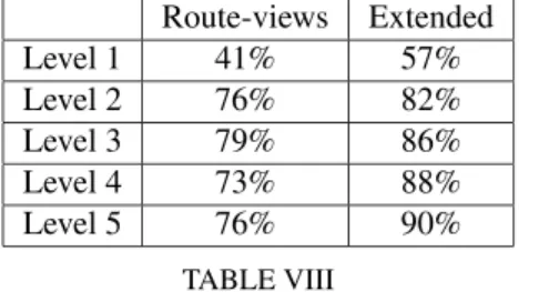
Route-views Extended Level 1 41% 57% Level 2 76% 82% Level 3 79% 86% Level 4 73% 88% Level 5 76% 90% TABLE VIII
PERCENTAGE OF NODES IN THE GIANT COMPONENT IN THE FIRST 5
LEVELS OF THE DECOMPOSITION
edges than obtained from theroute-viewsdata set alone. We
actually downloaded instances of the AS topology (from [1]) created using the augmented data set as part of the study done by [8] dating from March, 2001.
Let us now apply our decomposition techniques to both these graphs. We observe that the main difference in the decompo-sition is that, across all levels of decompodecompo-sition, the extended topology has a larger relative size of the giant component as compared to the route-views topology. For example, in the first level of decomposition 57% of all nodes are in the giant
compo-nent in theExtendedtopology as compared to 41% in the
Route-viewstopology. Let us examine why this is the case. Firstly, as
pointed earlier, several extra edges in theExtendedtopology are
links between a multi-homed AS and its providers. It is possible that an AS may spread such links across providers in different tiers. Thus, as an example, upon removal of the highest 1% de-gree nodes, a customer AS may lose some of its provider links, but could continue to remain connected to the giant component by virtue of also having links with lower-degree (or lower-tier) ASes. In order to verify this notion, we looked into what
per-centage of nodes with degree≤10are connected solely to the
highest 1% degree nodes. In the case of theRoute-views
topol-ogy, nearly 46% of such nodes were connected only the highest
degree nodes, and this falls to 39% of nodes in theExtended
topology. Also, another source of the extra edges are peer-peer links between lower-tier ASes. The existence of such links fur-ther increases the resiliency of the giant component across all levels.
Finally, we examined the degree distribution of nodes in the
giant components at different levels of decomposition. We
found that, similar to theRoute-viewstopology, the degree
dis-tribution in theExtendedgraph follows the Pareto in the body
and the Exponential distribution for the tail, as is shown in Fig-ure 9. We have statistically verified this hypothesis by doing goodness-of-fit tests for these distributions.
To summarize, after applying our decomposition techniques on the augmented data set we observe the decomposition of the
Extendedtopology remains qualitatively and statistically
simi-lar to theRoute-viewstopology despite some quantitative
dif-ference in the size of giant connected components at different levels of decomposition.
B. Decomposition over different PLRG constructions
A question we consider is if the similarity of the decompo-sition in the three family of graphs is simply a byproduct of
100 102 10−4 10−3 10−2 10−1 100 x: log10(degree) Pr(X > x) AS Pareto, a = 1.18 Exp, l = 7.0 100 101 102 10−4 10−3 10−2 10−1 100 x: log10(degree) Pr(X > x) AS Pareto, a = 1.05 Exp, l = 5.0 100 101 102 10−4 10−3 10−2 10−1 100 x: log10(degree) Pr(X > x) AS Pareto, a = 1.12 Exp, l = 2.9
Fig. 9. Fitting Pareto and Exponential distributions to body and tail of node
degrees in the giant CC at first 3 levels of decomposition in theExtended
topol-ogy
the fact that they have the same degree distribution? In order to answer this question, we construct three different types of PLRG graphs, each starting with the same node degree distribu-tion, but with nodes interconnected differently. The first type of graph is the standard PLRG graph in which nodes of a certain degree are randomly matched with each other. In the second type of graph (termed PLRG-ascending), we connect nodes in the following way. We start with the highest-degree node, and enforce the policy that this node give priority to connect with the lowest-degree nodes, until its degree is exhausted. We then move on to the next highest-degree node. In this construction, nodes with high degrees are sparsely connected with each other. The third type of graph (termed PLRG-descending) is con-structed in the reverse manner as the former - a higher priority is given for nodes with high degrees to connect with each other. Upon applying our decomposition technique to these graphs, we observe that both PLRG-ascending and PLRG-descending show a very different decomposition structure than the standard PLRG graph. At the first level of decomposition itself, these graphs break down into many connected components, with no existence of a giant component. This simple example illustrates that replicating the degree distribution of a graph is not suffi-cient to reproduce its decomposition characteristics.
PLRG PLRG-ascending PLRG-descending Level 0 50% 1% 22% Level 1 88% 95% 92% Level 2 90% 97% 95% Level 3 91% 97% 96% Level 4 90% 98% 95% TABLE IX
PERCENTAGE OF NODES IN THE LARGEST CONNECTED COMPONENT IN THE FIRST FIVE LEVELS OF DECOMPOSITION
C. Decomposition with different values ofα
Until now in our decomposition, we have used a fixed value
ofα = 0.01, as the fraction of nodes to be removed in each
stage of the decomposition. In Table X we present results from
carrying out the decomposition for different values ofα.
Be-low, we present only the figures for the relative size of the gi-ant component in the first level of decomposition, we have ob-served similar trends for lower levels. We note that, except for the Waxman graph, the size of the giant component decreases
with an increase inα, and after a certain point, there no longer
exists a “giant” component.
α AS Graph PLRG GLP Waxman 0.005 59% 57% 33% 99% 0.010 45% 50% 21% 99% 0.020 14% 38% 1% 98% 0.030 3% 29% 1% 97% 0.040 1% 17% 1% 96% 0.050 1% 6% 1% 94% TABLE X
PERCENTAGE OF NODES IN THE LARGEST CONNECTED COMPONENT IN DECOMPOSITION LEVEL1WITH VARYINGα