Sharif University of Technology
Scientia IranicaTransactions E: Industrial Engineering www.scientiairanica.com
Population-based metaheuristics for R&D project
scheduling problems under activity failure risk
M. Ranjbar
, H. Validi and R. Fakhimi
Department of Industrial Engineering, Faculty of Engineering, Ferdowsi University of Mashhad, Mashhad, Iran. Received 20 May 2014; received in revised form 10 January 2015; accepted 15 June 2015
KEYWORDS Project scheduling; Risk;
Scatter search; Genetic algorithm.
Abstract. In this paper, we study scheduling of R&D projects in which activities may to be failed due to the technological risks. We consider two introduced problems in the literature referred to as R&D Project Scheduling Problem (RDPSP) and Alternative Tech-nologies Project Scheduling Problem (ATPSP). In both problems, the goal is maximization of the expected net present value of activities where activities are precedence related and each of them is accompanied with a cost, a duration, and a probability of technical success. In RDPSP, a project payo is obtained if all activities are succeeded, while in ATPSP, if one of activities is implemented successfully, the project payo is attained. We construct a solution representation for each of these problems and construct two population-based metaheuristics including scatter search algorithm and genetic algorithm as solution approaches. Computational experiments indicate scatter search outperforms genetic algorithm and also available exact solution algorithms.
© 2016 Sharif University of Technology. All rights reserved.
1. Introduction
In a lot of industries, projects are subject to con-siderable uncertainty due to various causes. Factors inuencing the completion date of a project include activities that are required but were not identied beforehand, activities taking longer than expected, activities that need to be redone, resources being unavailable when required, late deliveries, etc. In Research and Development (R&D) projects, activities may also fail altogether, for instance because the new technology under study does not perform as anticipated or because a toxicity test is not passed (in case of drug development). This risk is often referred to as technical risk. We consider the main sources of uncertainty
*. Corresponding author. Tel.: +98 51 38805092 E-mail addresses: m [email protected] (M. Ranjbar); [email protected] (H. Validi);
[email protected] (R. Fakhimi)
in R&D projects, namely, the possibility of activity failure.
De Reyck et al. [1] introduced the modular R&D project scheduling as an R&D project consisting of several modules. In this problem, each module contains one or more activities that pursue a homogeneous target, for instance, representing repeated trials or technological alternatives. Each activity has a cost, a duration, and a Probability of Technical Success (PTS). It should be mentioned that in some references, such as [2], the term \alternative" has been used in-stead of \activity" in the ATPSP, but we use \activity" in this research. A module is successful when at least one of its included activities succeeds. Successful completion of the whole project requires successful completion of all the modules; project success equates with receiving a project payo (cash inow). In their model, they made a number of simplifying assump-tions, including unlimited resources and no explicit consideration of the uncertainty in activity durations or project cash ows.
In this paper, we consider two problems: the RDPSP and the ATPSP. These two problems were introduced by De Reyck and Leus [3] and each of them is a special case of the modular R&D project scheduling problem. The goal is maximization of the expected Net Present Value (eNPV) in both the aforementioned problems. The RDPSP is a single-activity-module project scheduling problem in which each module consists of only one activity and successful completion of the whole project requires successful completion of all the activities. The ATPSP is a single-module project scheduling problem in which the project consists of one module and technical success of an activity leads to obtaining the project payo.
The literature on project scheduling is vast and interested readers are referred to recent literature sur-veys in this eld (e.g. [4,5]). In this study, we focus only on R&D project scheduling problems. The main topic of interest in the literature surveys on the scheduling under uncertainty is duration uncertainty, sometimes complemented with uncertain resource availabilities [6-8]. In this paper, we incorporate the concepts of activity success or failure into the scheduling decisions. A branch-abound (B&B) algorithm was developed for the RDPSP by De Reyck and Leus [3]. A similar model is tackled by [9,10] in which the scheduling of failure-prone new-product-development testing tasks is studied when non-sequential testing is admitted. The concept of modular projects is hinted at [1], but the authors do not develop any solution procedure. This re-search work has been continued by Creemers et al. [11] in which modular projects by considering the impact of activity duration variability on the project's value are studied. Also, Ranjbar and Davari [2] develops a B&B algorithm for the ATPSP. In all of the foregoing references, the resource constraint has not been taken into account, but recently, Coolen et al. [12] considered scheduling modular projects on a bottleneck resource. They described various policy classes, established the relations among them, and developed exact algorithms to optimize two dierent classes.
Closely related to the model developed in this paper is the work on sequential testing, in which a series of tests is to be performed to diagnose a system (i.e., to know its state, which usually is either `working' or `failing'). A solution in this setting is an inspection strategy, which is specied on the basis of the state of the already inspected components. Each component is to be inspected next, or halts if it is able to recognize the correct state of the system. Reviews of this body of literature can be found in [13,14]. The main dierences with our scheduling problem is that the inspections will continue as long as the state of the system is not known, whereas we allow the project to be aborted preliminarily if this is better for the project's value.
One of the most important weaknesses in the
previous research works on R&D project scheduling problems is that the developed solution approaches are applicable only for small-scale test instances. Thus, developing solution approaches which can solve large-scale and practical problems is really a research gap. To overcome this crisis, in this research, we construct ecient solution approaches.
The contributions of this article are twofold:
1. We develop representations of two solutions for the RDPSP and ATPSP, respectively;
2. We develop two population-based metaheuristic algorithms including two dierent combining meth-ods and customized repairing and local search procedures to solve both problems.
The remainder of this paper is organized as follows. Section 2 contains formal denition and formulation of the RDPSP and ATPSP. Our scatter search algorithm along its components is described in Section 3 and computational performance is evaluated in Section 4. Finally, Section 5 contains a summary, some conclu-sions, and ideas for further research.
2. Formulation of the problems
The objective of RDPSP and ATPSP is to maxi-mize eNPV of the project by constructing a project schedule specifying when to execute each activity. In the RDPSP (ATPSP), the nal project payo is only achieved when all activities are (one activity is) successful, and the project is terminated as soon as an activity fails (succeeds). Activity success or failure is revealed at the end of each activity. Consequently, in the RDPSP (ATPSP), each activity will start only if all the activities scheduled to nish earlier have a positive (negative) outcome and hence, in the objective function, the activity cash ows are weighted by the probability of joint success (failure) of all its scheduled predecessors. We do not consider resource constraints and duration uncertainty, and consider the PTS of the dierent tasks as independent. The parameters that are used throughout the paper are dened in Table 1.
Without loss of generality, we assume activity 0 to be a dummy activity representing project initiation and be the predecessor of all other activities with c0= d0=
0 and p0 = 1. Activity n + 1 is also a dummy activity
representing project completion and is a successor of all other activities. We assume that di> 0 for all
non-dummy activities. A deadline is imposed on project completion because we require that sn+1 . This
deadline is needed because optimization will try to push the start times of activities to innity if the optimal eNPV of a particular problem instance is negative.
A schedule s is feasible if it respects the con-straints imposed by A. In the RDPSP (ATPSP), the
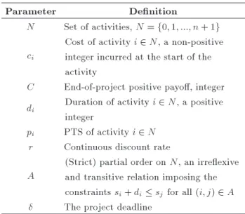
Table 1. Denitions of parameters.
Parameter Denition
N Set of activities, N = f0; 1; :::; n + 1g ci
Cost of activity i 2 N, a non-positive integer incurred at the start of the activity
C End-of-project positive payo, integer di Duration of activity i 2 N, a positive
integer
pi PTS of activity i 2 N
r Continuous discount rate A
(Strict) partial order on N, an irreexive and transitive relation imposing the constraints si+ di sjfor all (i; j) 2 A
The project deadline
objective is to maximize the project's eNPV , so the cost of each activity is weighted by the probability of joint success (failure) of the already nished activities. We represent each schedule by a vector of start times s = (s0; s1; :::; sn+1) where si is a non-negative integer
and indicates the start time of activity i. We also consider f = (f0; f1; :::; fn+1) as the vector of nish
times, where fi = si+ di, indicates the nish time of
activity i.
The RDPSP can now be formulated as the follow-ing non-linear integer programmfollow-ing model:
max g1(s) = n
X
i=1
ciexp( rsi)
Y
j2F BA(si)pj
+ C exp( rsn+1)
Yn j=1pj;
subject to:
si+ di sj 8(i; j) 2 A;
sn+1 ;
si2 Z+ 8i 2 N:
In the objective function g1(s) which indicates eNPV
of schedule s, F BA(si) indicates the set of activities
which are nished before or at the start time of activity i. g1(s) includes two main terms in which exp(:) shows
exponential function. The rst term indicates the expected value of costs while the second term shows the expected value of revenue. The rst constraint of the model indicates the nish-to-start precedence relations among activities imposed by set A. The second constraint implies that dummy end activity n + 1 must be nished before or at the given deadline.
The last constraint shows that all start times are non-negative integers (Z+ indicates the set of non-negative
integers).
The formulation of ATPSP is similar to that of RDPSP, but instead of g1(s), we use g2(s), where:
g2(s) = n
X
i=1
0
@exp( rsi)ci
Y
j2F BA(si)
(1 pj)
1 A +CX t2NUF 0 @exp( rt) 0 @1 Y k2F A(t)
(1 pk)
1 A Y
j2F B(t)
(1 pj)
1 A
+C X
i:fi2NUF=
0
@exp( r(si+ di))pi
Y
j2F B(si+di)
(1 pj)
1 A : In g2(s), F B(fi) shows the set of activities which are
nished before nish time of activity i. In addition, NUF shows the set of non-unique nish times such that every t 2 NUF is equivalent to the nish time of at least two activities. The set of activities, which are nished at t 2 NUF, are shown by F A(t). In addition, F B(t) shows the set of activities which are nished before time instant t. g2(s) includes three main terms in which
the rst term represents the expected costs in which Q
j2F BA(si)(1 pj) indicates the probability of joint
failure of all activities nished before or at the start time of activity i. We assume that if in a schedule for two activities, j 2 N, we have fj = si, then activity
i will start if activity j fails. The summation of two other terms in g2(s) indicates the expected revenue.
The second term displays the expected revenue for the activities whose nish times belong to NUF. In this formula, (1 Qk2F A(t)(1 pk)) shows the probability
of succeeding at least one of the activities nished at time instant t. Moreover, Qj2F B(t)(1 pj) indicates
the probability of joint failure of all activities nished prior to the time instant t. Finally, the last term species the expected revenue for the activities with unique nish times. In this formula,Qj2F B(si+di)(1 pj) represents the probability of joint failure of all
activities nished prior to the completion time of activity i.
3. Schedule representation
Our heuristic algorithms use a schedule representation to encode a schedule. Although there are various approaches for schedule representation of the clas-sic resource-constrained project scheduling problem (see [15]), there is not any solution representation for RDPSP and ATPSP in the literature. We develop two schedule representations for the RDPSP and ATPSP based on the solution approaches made by [2,3], re-spectively.
3.1. Schedule representation for the RDPSP Based upon solution of [3], RDPSP is solved in two phases. In the rst phase, a feasible extension E of A, which updates sets F BA(si) for some i 2 N, is
produced. Then, function g1(:) is optimized subject
to new precedence constraints, which constitutes the second phase. If all feasible extensions of A will be implicitly or explicitly enumerated, nding an optimal schedule for RDPSP is guaranteed. The second phase (optimization for the given new precedence constraints) amounts to project scheduling with eNPV objective without resource constraints (see [16]). We consider the case in which all activity cash ows during the development phase are negative, which is typical for R&D projects. In this case, the scheduling problem is easily solved because all intermediate cash ows are non-positive: Each activity can be scheduled to end at the earliest of the start times of its successors in E. Depending on whether the corresponding eNPV is positive or negative, we set s0 = 0 or sn+1 = ,
respectively. Based upon this solution approach, we represent each schedule of the RDPSP by a set of pairs f(i; j) : 8(i; j) =2 Ag. In other words, we consider pairs of activities for which there is not any directed path between them in the project network. For each (i; j) =2 A, we consider three dierent scenarios: (i ! j); (i j), and (ijjj), where (i ! j) implies sj si+di
and (ijjj) implies jointly relations si + di > sj and
sj+ dj > si. In other words, relation (i ! j) indicates
that activity j can start after the end of activity i due to the information ow from i to j. Also, relation (ijjj) designates that activities i and j will overlap in execution. Each schedule representation is feasible i there is no cycle in the corresponding project network. When a feasible schedule representation is generated, we schedule all activities based on their latest possible start times, calculated based on the Critical Path Method (CPM). Now, if there is a pair (i; j) =2 A for which we have (ijjj) in our schedule representation, but we know sj si+ di on the basis of start times
values obtained from the Latest Start Schedule (LSS), we change (ijjj) into (i ! j).
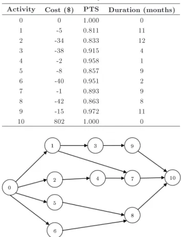
As an example, we consider a project with 11 activities as represented in Figure 1.
Other project data are given in Table 2. In this example, we assume a discount rate of 5% per month and the project deadline is 67 months. Consider the following feasible schedule representation:
f(1 ! 2); (1jj4); (1jj5); (1jj6); (1jj8); (2jj3);
(2 5); (2jj6); (2jj8); (2jj9); (3jj4); (3jj5); (3jj6); (3jj7); (3jj8); (4jj5); (4jj6); (4jj8); (4jj9); (5jj6); (5jj7); (5jj9); (6jj7); (6jj9); (7jj8); (7jj9); (8jj9)g:
Table 2. Project data.
Activity Cost ($) PTS Duration (months)
0 0 1.000 0
1 -5 0.811 11
2 -34 0.833 12
3 -38 0.915 4
4 -2 0.958 1
5 -8 0.857 9
6 -40 0.951 2
7 -1 0.893 9
8 -42 0.863 8
9 -15 0.972 11
10 802 1.000 0
Figure 1. Network of the example project.
Figure 2. Optimal schedule of the RDPSP.
The corresponding LSS of this representation is pre-sented in Figure 2, which is also optimal schedule with eNPV of $11.37. Using information obtained from the LSS, this representation will be changed as follows:
f(1 ! 2); (1 ! 4); (1jj5); (1 ! 6); (1 ! 8); (2jj3); (2 5); (2 ! 6); (2 ! 8); (2jj9); (3 ! 4); (3 5); (3 ! 6); (3 ! 7); (3 ! 8); (4 5); (4jj6); (4 ! 8); (4jj9); (5 ! 6); (5 ! 7); (5 ! 9); (6jj7); (6jj9); (7jj8); (7jj9); (8jj9)g:
This change implies that the relation between solution space and solution representation space is not one to one, because several solution representations may correspond to an identical schedule.
Figure 3. Optimal schedule of the ATPSP.
3.2. Schedule representation for the ATPSP In the ATPSP, we use a direct representation and show each schedule by its vector of start time s = (s0; s1; :::; sn+1). Ranjbar and Davari [2] dene the
concurrency property and prove that there is an op-timal solution for each instance of the ATPSP which is concurrent. Based on this property, the start time or nish time of each activity, which is dened as an event, is concurrent with the start time or nish time of at least another activity. Thus, our solution representation for the ATPSP is subject to the concurrency property. Figure 3 presents the optimal schedule of the ATPSP with eNPV of $671.77 based on the example project depicted in Figure 1. We represent this schedule as s = (0; 2; 28; 13; 40; 2; 0; 41; 17; 17; 50).
4. Solution approaches
In this section, we develop two metaheuristics including scatter search and genetic algorithm. These two algorithms are both population-based and we have considered some similar or common operators for them, but their overall structures are dierent.
4.1. A scatter search algorithm
Scatter Search (SS) was developed by Glover and Laguna [17] as a heuristic algorithm for integer pro-gramming models. In this algorithm, solutions are generated randomly such that they cover most parts of the solution space. Similar to tabu search algorithm, SS has diversication and intensication procedures to enhance its eciency [18]. For a brief and general introduction to SS, we refer the readers to [19]. Scatter search algorithm has been used in previous research on scheduling problems, such as [20-23].
Figure 4 shows the main structure of our SS algo-rithm as a owchart for both the RDPSP and ATPSP in which some operators have dierent procedures for each problem. In the rst step, an initial population P containing jP j solutions is generated using the initial population generation method, described in Section 4.1. If the termination criterion, a given time limit, is met, the SS algorithm stops; otherwise, it continues. In the second step, the reference set RefSet, including b elite solutions of P , is constructed using the reference set building method, described in Section 4.2. The solutions of RefSet are called reference solutions. Next, the NewSubsets, each of them containing two reference solutions, are generated.
In this stage, the best solution of the current
Figure 4. Flowchart of the SS algorithm.
population is kept and the other solutions are removed. Subsequently, two solutions of each subset, called parents solutions and shown by (sf; sm), are selected
and the combining operator, described in Section 4.3, is applied to them. We consider sfand smas the father
and mother solutions, respectively. Since it is possible that generated schedules ss and sd are infeasible, we
apply the repairing operator, described in Section 4.5, to them. Then, the objective functions of schedules ss, and sd are evaluated and the better schedule is
selected to be improved by the local search operator, described in Section 4.6, with probability of pls. The
selected schedule will be added to the population P after improvement by the local search operator. After selection of all pairs (sf; sm) in NewSubsets, the size of
population P will be 2jP j. In this stage, population P will be updated by removing jP j worse schedules from P .
Figure 5. Pseudo-code of the initial population generation method for the ATPSP.
4.1.1. Initial population generation method
Each member of the initial population P in the RDPSP is generated randomly. For this purpose and for each pair of activities (i; j) =2 A, we select one of the three cases (i ! j); (i j), or (ijjj), randomly. Since the generated project network may include cycle and be infeasible, we use the repairing procedure expressed in Section 4.4.
Also, each member in the initial population of ATPSP is a random solution and is created by the method, illustrated in Figure 5, by pseudo-code. In this approach, activities are added one by one to a partial schedule s. EA(s) indicates the set of eligible activities, initialized by all activities which do not have any predecessor. Also, SA(s) represents the set of scheduled activities initialized as an empty set.
After the initialization step, we follow an iterative while-loop to construct a random solution. In each iteration, an individual activity is added to the partial schedule s. At step 3, one of the eligible activities, shown by j, is selected randomly. Next, eligible start times for activity j in schedule s, noted by ESj(s), are
calculated based upon concurrency property. Next, one of the eligible events for the start time of activity j is chosen, randomly, and activity j starts in that time. It should be noticed that for each activity j which does not have any predecessor (successor), t = 0(t = dj) is always a valid start time. However, in the next
step, sets EA(s) and SA(s) are updated. In order to update set EA(s), activity j should be removed from EA(s) and all activities i 2 Suc(j) for which P red(i) SA(s) should be added to EA(s), where Suc(j) and P red(j) indicate the set of successors and predecessors of activity j, respectively. Also, set SA(s) is updated simply as SA(s) = SA(s) [ j.
4.1.2. Reference set building and subset generation methods
The reference set, RefSet, is a collection of both high quality solutions and diverse solutions that are used to generate new solutions by way of applying the combin-ing, repaircombin-ing, and local search operators. We construct RefSet based on the method applied for construction of RefSet1 of scatter search in [22]. We select the
solution with the smallest objective function, shown
as s1, as the rst member of RefSet and remove it from
P . The next best solution s in P is chosen and added to RefSet only if Dmin(s) th dist, where Dmin(s) is
the minimum of the distances of solution s to the all solutions currently in RefSet. Also, th dist indicates a threshold distance. In the RDPSP, the dierence between two solutions equals the number of dierent ordered activities (i; j) =2 A in two solutions divided by the number of unordered pairs of activities. Also, in the ATPSP, the dierence between two solutions equals the number of dierent start times for identical non-dummy activities in two solutions divided by the number of non-dummy activities. Thus, the dierence between every two solutions changes in range [0,1]. This process is repeated until b members are chosen for RefSet. Whenever no qualied solution can be found in the population, the RefSet is completed with random solutions generated based on the initial population generation method. For these members of RefSet, the condition of minimum threshold distance is ignored.
In the next step, NewSubsets are generated con-sisting of all pairs of reference solutions. The pairs in NewSubsets are selected at a time in lexicographical order and the combining, repairing, and local search operators are applied to generate one trial solution. Thus, the size of P will be always (b2 b)=2 + 1, where
one more solution shows the best solution so far. 4.1.3. Combining operators
After the selection of parents sf and sm from
New-Subsets, a combining operator combines these two schedules to generate children ss and sd, respectively.
We use two dierent methods as combining operators. We consider the Combining Operator 1 (CO1) as the well-known two-point crossover operator in which the crossing points are determined randomly. If we consider cp1and cp2as the crossing points where cp1<
cp2, the elements of ssare identical to the elements of
sf, except those placed in positions [cp
1; cp2] for which
elements of smare used to construct ss. Generation of
sd is similar to generation of ss but with exchanging
the roles of sf and sm. For example, consider the two
following schedule representations sf and sm for the
RDPSP and assume cp1= 8 and cp2= 19.
sf = f(1jj2); (1 ! 4); (1jj5); (1 ! 6); (1 ! 8);
(2 ! 3); (2 ! 5); (2 ! 6); (2 ! 8); (2 ! 9); (3jj4); (3jj5); (3 ! 6); (3 ! 7); (3 ! 8); (4jj5); (4 ! 6); (4 ! 8); (4 ! 9); (5 ! 6); (5 ! 7); (5jj9); (6jj7); (6jj9); (7jj8); (7jj9); (8jj9)g;
sm= f(1jj2); (1jj4); (1jj5); (1 6); (1 ! 8);
(2 ! 3); (2 ! 5); (2 6); (2 ! 8); (2 ! 9); (3 4); (3jj5); (3 6); (3jj7); (3 ! 8); (4 ! 5); (4 6); (4 ! 8); (4 ! 9); (5 6); (5jj7); (5jj9); (6 ! 7); (6 ! 9); (7 ! 8); (7 ! 9); (8jj9)g:
By applying the two-point crossover operator to sf and
sm, the two following schedule representations sm and
ssare obtained.
ss= f(1jj2); (1 ! 4); (1jj5); (1 ! 6); (1 ! 8);
(2 ! 3); (2 ! 5); (2 6); (2 ! 8); (2 ! 9); (3 4); (3jj5); (3 6); (3jj7); (3 ! 8); (4 ! 5); (4 6); (4 ! 8); (4 ! 9); (5 ! 6); (5 ! 7); (5jj9); (6jj7); (6jj9); (7jj8); (7jj9); (8jj9)g;
sd = f(1jj2); (1jj4); (1jj5); (1 6); (1 ! 8);
(2 ! 3); (2 ! 5); (2 ! 6); (2 ! 8); (2 ! 9); (3jj4); (3jj5); (3 ! 6); (3 ! 7); (3 ! 8); (4jj5); (4 ! 6); (4 ! 8); (4 ! 9); (5 6); (5jj7); (5jj9); (6 ! 7); (6 ! 9); (7 ! 8); (7 ! 9); (8jj9)g:
For the ATPSP, if we refer to parents as s0f and s0m
and assume cp1 = 4 and cp2 = 7, by applying the
two-point crossover operator to s0f and s0m, we obtain
ospring schedules s0s and s0d as follows.
s0f = (0; 0; 11; 18; 23; 2; 23; 24; 25; 22; 33) and
s0m= (0; 2; 0; 17; 21; 13; 0; 24; 25; 22; 35);
s0s= (0; 0; 11; 17; 21; 13; 0; 24; 25; 22; 33) and
s0d = (0; 2; 0; 18; 23; 2; 23; 24; 25; 22; 35):
Also, we design the Combining Operator 2 (CO2) based on a path-relinking algorithm developed by Ranjbar et al. [22]. The CO2 gets two parent solutions as inputs
and generates a set of child solutions as follows. In this method, the elements of sf and smare compared
from left to right respectively. The rst element of sf which diers from the corresponding element of sm
is changed such that to be identical with sm. This
change creates a new solution (s1). For example, in
the RDPSP, the two following solutions sf and sm
dier in the second element, indicating the precedence relation between activities 1 and 4. Thus, s1 is a
copy of sf, but in which relation (1 ! 4) has been
changed to (1jj4), taken from sm. Next, we nd the rst
dierent element between s1 and sm which is related
to activities 1 and 6. Using changing relation (1 ! 6) to (1 6), s2 is generated from s1. This process
is repeated until we reach sm. In this example, 13
dierent solutions are generated. The CO2 randomly selects two solutions, one solution from the rst half of all the generated solutions and another one from the second half. These two solutions are considered as children solutions.
sf = f(1jj2); (1!4); (1jj5); (1!6); (1!8);
(2!3); (2!5); (2!6); (2!8); (2!9); (3jj4); (3jj5); (3!6); (3!7); (3!8); (4jj5); (4!6); (4!8); (4!9); (5!6); (5!7); (5jj9); (6jj7); (6jj9); (7jj8); (7jj9); (8jj9)g; s1= f(1jj2); (1jj4); (1jj5); (1!6); (1!8); (2!3);
(2!5); (2!6); (2!8); (2!9); (3jj4); (3jj5); (3!6); (3!7); (3!8); (4jj5); (4!6); (4!8); (4!9); (5!6); (5!7); (5jj9); (6jj7); (6jj9); (7jj8); (7jj9); (8jj9)g;
s2= f(1jj2); (1jj4); (1jj5); (1 6); (1!8); (2!3);
(2!5); (2!6); (2!8); (2!9); (3jj4); (3jj5); (3!6); (3!7); (3!8); (4jj5); (4!6); (4!8); (4!9); (5!6); (5!7); (5jj9); (6jj7); (6jj9); (7jj8); (7jj9); (8jj9)g;
s3= f(1jj2); (1jj4); (1jj5); (1 6); (1!8); (2!3);
(2!5); (2 6); (2!8); (2!9); (3jj4); (3jj5); (3!6); (3!7); (3!8); (4jj5); (4!6);
(4!8); (4!9); (5!6); (5!7); (5jj9); (6jj7); (6jj9); (7jj8); (7jj9); (8jj9)g;
...
s13= f(1jj2); (1jj4); (1jj5); (1 6); (1!8); (2!3);
(2!5); (2 6); (2!8); (2!9); (3 4); (3jj5); (3 6); (3jj7); (3!8); (4!5); (4 6); (4!8); (4!9); (5 6); (5jj7); (5jj9); (6!7); (6!9); (7!8); (7 ! 9); (8jj9)g; sm= f(1jj2); (1jj4); (1jj5); (1 6); (1!8); (2!3);
(2!5); (2 6); (2!8); (2!9); (3 4); (3jj5); (3 6); (3jj7); (3!8); (4!5); (4 6); (4!8); (4!9); (5 6); (5jj7); (5jj9); (6!7); (6!9); (7!8); (7!9); (8jj9)g:
The CO2 method follows the same strategy for the ATPSP, but it deals with numbers instead of precedence relations.
4.1.4. Repairing operator
It is possible that the ospring schedules generated by the initial population generation method or by the crossover operator are infeasible. In order to overcome this problem, we repair each schedule representation after its generation. For this purpose, we generate a random sequence of all pairs (i; j) =2 A and then check the feasibility of the network based on this sequence. Whenever the infeasibility condition is found due to a relation like (i ! j), we change it as (i j). As an example, consider the schedule representation ss
introduced in Section 4.3. Since there is loop 2 ! 5 ! 6 ! 2 in the corresponding project network of this schedule representation, we should change precedence relation (5 ! 6) as (5 6).
The repairing operator for the ATPSP includes two steps. The rst step is applied to infeasible solutions for the purpose of making them feasible while the second step is applied to the solutions which are not subject to the concurrency property. In the rst step in which the precedence constraints are investigated, for each activity i 2 N, if si < max
j2P red(i)ffjg, we
set si = max
j2P red(i)ffjg. In the second step of the
repairing method, for each activity i 2 N in which si =2 ESi, we shift the activity to the direction that has
more positive or less negative impact on the objective
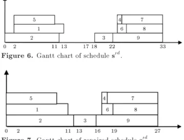
Figure 6. Gantt chart of schedule s0d.
Figure 7. Gantt chart of repaired schedule s0d.
function by the minimum amount required such that we have si 2 ESi. For example, consider schedule
representation s0d, shown in Section 4.3 and depicted
in Figure 6.
In this schedule, at rst, activity 2 is scheduled which is concurrent with event t = 0. Then, activities 1 or 5 are scheduled where none of them is concurrent with available events. Thus, we change s1= 0 and s5=
0. Then, activities 3, 4, 5, 6, 7, 8, and 9 are shifted to the left such that the precedence relations among them is kept and s3 = f2 = 12. Finally, we obtain schedule
representation s0d = (0; 0; 0; 12; 17; 0; 17; 18; 19; 16; 27),
depicted in Figure 7. 4.1.5. Local search operator
A local search operator is applied to each children schedule with the probability of pls to enforce search
intensication. For the RDPSP, this operator changes each unordered pair (ijjj) as (i ! j) and (i j) if each of these directions does not make the project network infeasible. For each direction of each unordered pair of activities, the eNPV is calculated. It should be noticed that the impact of each change is evaluated while other unordered pairs of activities are not changed. The current schedule is replaced with the best schedules found in the aforementioned alterations and the local search procedure is repeated.
Similarly, for the ATPSP, we change the start times of activities instead of direction of the unordered pair of activities. For this purpose and for a given schedule s, we should rst calculate the ESi(s) based
upon concurrency property for each activity i 2 N. Then, siis changed to each time t 2 ESi(s) while start
times of other activities are kept the same. Finally, the impact of each change is evaluated and the best found solution is replaced with the current solution and this procedure is repeated. Both the foregoing local search procedures are stopped whenever no improvement is obtained anymore.
4.2. A genetic algorithm
The Genetic Algorithm (GA) was developed by [24] based on the biological evolution idea for solving compound optimization problems. GA has been widely used in optimization problems [25]. Our GA starts with generation of the initial population P with size of jP j. Each element (solution) of the P is gen-erated by the initial population generation method, described in Section 4.1.1. In order to develop a new element P , each element of the current population, which is considered as the father schedule (sf), is
mated randomly with other element of the population, considered as the mother schedule (sm). They
con-stitute a couple and each couple generates two child schedules, considered as the son schedule (ss) and the
daughter schedule (sd). The child generation process
is performed using three operators, i.e. combining, mutation, and local search. The combining and local search operators have been presented in Sections 4.1.3 and 4.1.5. The mutation operator selects 100pmut
percent of cells of each solution and changes them randomly to other dened states. Since the gener-ated child solutions may be infeasible, the repairing operator, described in Section 4.1.4, is also applied in the necessary cases to make the generated solutions feasible.
The child with the better eNPV is chosen as the child (sc) of the parents and is improved by the
local search operator with probability of pls. Next,
it is added to the end of P . Then, the population, consisting of the 2jP j elements, is updated by deleting half of its elements in such a way that the best individuals will appear in the population more than those with a worse eNPV value, emulating the \survival of the ttest" principle of nature. To that purpose, we delete population elements using a biased random sampling method in which the deletion probability of each element is inversely proportional to its eNPV. In order to prevent drop of the best-found schedule so far, we will never delete it from the population. This procedure will be continued until the termination criterion is met.
5. Computational results 5.1. Benchmark problem set
All coding was implemented in the Visual C++ 6.0 en-vironment; all experiments were run on a PC Pentium IV 3 GHz processor with 1024 MB of internal memory. For the RDPSP, we used the test sets of [3] including 420 test instances in which n = 10; 15; 20; 25; 30; 35; 40 and OS = 0:25; 0:5, and 0:75 where OS is the Order Strength, the number of precedence-related activity pairs divided by the theoretically maximum number of such pairs in the network [26]. For each com-bination of n and OS, 20 test instances were
gen-erated varying in the durations of activities, costs, and PTSs: durations and costs are realizations of (independent) discrete uniform random variables on the intervals [1; 15] and [ 50; 0], respectively, and the PTS-values are with uniform probability chosen from [80%; 100%].
Also, for the ATPSP, we used test sets generated by De Reyck and Leus [3] including 60 test instances in which they chose n = 6; 8; 10; 12 and OS = 0:4; 0:6, and 0:8. For each combination of n and OS, they generate ve test instances. Moreover, durations and costs are realizations of (independent) discrete uniform random variables on the intervals [1; 10] and [ 100; 10], respectively, and the values of PTS are with uniform probability chosen from [50%; 100%]. Unless mentioned otherwise, we set r = 0:05.
In order to compare the eciency of our developed algorithms, we generated two large-scale test sets including 120 test instances of RDPSP with n = 50; 100 and 30 test instances of ATPSP with n = 12; 15. 5.2. Setting of parameters
Using Design Of Experiments (DOE) technique and based on hard test instances of the RDPSP and ATPSP, we set the SS's parameters pls, th-dist, jP j, and
b. For each time limit, we considered three levels for the rst three parameters as follows: pls = 0:01; 0:03,
and 0.05; th-dist = 0:2; 0:4, and 0.6; jP j = 10b; 15b, and 20b. Also, for each of time limits, T L = 1, 10, and 100, we considered three levels for parameter b as shown in Table 3.
For each time limit, we ran a 34 full factorial
design and found the results of Table 4.
Similarly, we set the parameters of GA as jP j, pls,
and pmut, as shown in Table 5.
Table 3. Levels of parameter b.
T L b
1 4, 6, 8 10 12, 14, 16 100 20, 30, 40 Table 4. Setting of parameter. T L b pls th-dist jP j
1 6 0.03 0.2 10b
10 12 0.03 0.4 10b
100 30 0.05 0.4 15b Table 5. Levels of the GA's parameter.
T L pls jP j
1 0.02 50 10 0.03 100 100 0.05 500
Table 6. Comparative results for combining methods.
Time limit T L = 1 second T L = 10 seconds T L = 100 seconds
Solution method SS+ CO1
SS+ CO2
GA+ CO1
GA+ CO2
SS+ CO1
SS+ CO2
GA+ CO1
GA+ CO2
SS+ CO1
SS+ CO2
GA+ CO1
GA+ CO2 RDPSP n = 50 23.81 21.44 26.46 24.67 8.18 5.61 9.00 6.14 0.16 0.04 0.20 0.14
n = 100 64.15 56.31 72.48 60.71 12.45 9.10 14.15 11.07 3.61 1.53 4.08 2.23 ATPSP n = 15 19.07 18.50 27.53 19.13 5.87 4.98 7.15 5.21 0.01 0.00 0.02 0.00 n = 20 29.64 24.71 36.38 26.09 8.13 7.13 8.92 7.18 2.07 1.81 2.37 1.96 TAPD 34.17 30.24 40.71 32.65 8.66 6.71 9.81 7.40 1.46 0.85 1.67 1.08
Table 7. Comparative results for the RDPSP. T L
T L = 1 second T L = 10 seconds T L = 100 seconds
SS+CO2 B&B SS+CO2 B&B SS+CO2 B&B
n
10 1.41(59) 0.00(60) 0.00(60) 0.00(60) 0.00(60) 0.00(60)
15 8.97(51) 6.34(53) 1.07(58) 1.04(58) 0.00(60) 0.00(60)
20 14.21(47) 8.94(51) 4.91(54) 2.84(57) 0.00(60) 0.00(60)
25 17.86(35) 29.94(20) 13.84(45) 26.84(25) 5.143(53) 19.02(35) 30 26.74(19) 35.83(13) 18.27(33) 31.11(19) 17.94(34) 28.60(23) 35 45.12(9) 51.59(5) 34.27(20) 37.61(16) 30.12(18) 34.08(20)
40 50.64(0) 59.71(0) 44.07(8) 54.88(3) 35.61(17) 41.37(14)
TAPD. (Avg#opt) 23.56(31.43) 27.48 (28.86) 16.63(39.71) 22.05(34) 12.69(43.14) 17.58(38.86)
5.3. Comparative computational results
As the termination criterion, we consider three time limits T L = 1, 10, and 100 seconds and run our SS, GA, and B&B procedures of [2,3] in the given time limits. The performance of our SS and GA for the RDPSP and ATPSP with two dierent combining methods have been summarized in Tables 5, 6, and 7, respectively. We report the Average Percent Deviation (APD) from the optimal solutions (or best known solutions). The best known solutions for the RDPSP with n = 10; 15; 20; 25; 30; 35; 40 and for the ATPSP with n = 6; 8; 10; 12 have been determined using B&B algorithms of [2,3]. For other test instances (large-scale test instance), the best found solutions have been obtained by SS or GA. The result of Table 6 shows the performance of SS and GA based on APD with two dierent combining methods of CO1 and CO2. This comparison has been made on the basis of large scale test instances which are more applicable for meta-heuristic algorithms. From Table 6 and based on the Total Average Percent Deviation (TAPD), we conclude that SS algorithms combined with CO2 has the best performance in both the RDPSP and the ATPSP. Also, it can be seen that with identical combining operator, SS outperforms GA in average. Thus, in the rest of
this paper, we compare only performance of SS+CO2 with exact solution algorithms.
The result of Table 7 shows that the developed SS+CO2 algorithm for the RDPSP dominates the B&B algorithms of [3]. In addition to APD, in each cell of this table, the number of times the optimal solution (#opt) is obtained is reported inside parenthesis. For test instances with n = 10, 15, and 20, the B&B algorithm has better performance than that of our developed SS+CO2, but for larger test instances, our SS+CO2 algorithm outperforms the B&B algorithm (in terms of both APD and #opt). The last row of Table 7 indicates the summarized results in terms of Total Average Percent Deviation (TAPD) and average number of optimal solutions (Avg#opt). This row indicates that SS+CO2 algorithm surpasses the B&B algorithm.
Similar to those of Table 7, the results of Table 8 indicate that our SS+CO2 algorithm outperforms the B&B algorithm of [2] in average and also for larger test instances (n = 10 and 12).
5.4. Sensitivity analysis
In this section, we analyze the impact of repairing and local search operators. On the basis of the
Table 8. Comparative results for the ATPSP. T L
T L = 1 second T L = 10 seconds T L = 100 seconds
SS+CO2 B&B SS+CO2 B&B SS+CO2 B&B
n
6 0.00(15) 0.00(15) 0.00(15) 0.00(15) 0.00(15) 0.00(15) 8 0.20(14) 0.17(13) 0.00(15) 0.00(15) 0.00(15) 0.00(15)
10 0.84(10) 2.44(4) 0.21(13) 0.59(8) 0.00(15) 0.05(14)
12 2.46(4) 3.35(0) 0.38(9) 2.32(3) 0.21(12) 1.86(5)
TAPD. (Avg#opt) 0.88(10.75) 1.49(8) 0.15(13) 0.73(10.25) 0.05(14.25) 0.48(12.25) Table 9. Impact of repairing and local search operators on the performance of SS+CO2.
n RDPSP ATPSP
10 15 20 25 30 35 40 6 8 10 12
SS+CO2/repairing 0.67 2.84 7.14 18.91 25.14 41.57 58.10 0.01 0.08 0.35 0.72 SS+CO2/local search 0.96 2.34 6.18 20.41 25.37 48.63 60.72 0.03 1.38 2.54 2.0
performance of SS+CO2, around 25% of precedence relations generated in RDPSP schedules were repaired (inversed). Also, around 35% of start times generated in ATPSP schedules were changed to nd feasible solutions. Moreover, in the second phase of the repairing operator of ATPSP, 18.5% of start times were changed because of the concurrency property. These results indicate that if we do not apply the repair-ing operator, a noticeable percent of solutions must be regenerated. To show eciency of the repairing operator, we run the SS+CO2 algorithm over both RDPSP and ATPSP without repairing operator by considering T L = 10 seconds. In this case, instead of each infeasible solution, a new random solution is generated until a feasible solution is found. In Table 9, the row titled by \SS+CO2/repairing" indicates the APD values while repairing operators have not been applied in the SS+CO2 algorithm. By comparing these outcomes with similar values reported in Tables 5 and 6, we nd that performance of the algorithm has decreased by as many as 6.65 and 4.8 percent for RDPSP and ATPSP, respectively.
Also, we run the SS+CO2 algorithm over both RDPSP and ATPSP without their corresponding local search procedures. The last row of Table 9 shows that the performance of SS+CO2 algorithm has decreased by around 7.8 and 6.47 percent for RDPSP and ATPSP, respectively.
6. Summary, conclusions, and further research In this paper we studied the project scheduling problem under the risk of failure of activities. We consid-ered two introduced problems in the literature: the RDPSP and ATPSP. We developed a scatter search
metaheuristic for the mentioned problems with especial components. Using available test sets in the literature, we compared the performance of our developed scatter search algorithm with those of the branch-and-bound algorithms, developed by Ranjbar and Davari [2] and De Reyck and Leus [3] for the ATPSP and RDPSP, respectively. The computational experiments indicated that our algorithm has better performance, especially for larger test instances.
For future research, we propose to consider the modular project scheduling and extend our algorithm for this new problem. In addition, developing new exact and metaheuristic algorithms with more ecient operators for the RDPSP and ATPSP can be interest-ing research topics.
Acknowledgments
This work is supported by Ferdowsi University of Mashhad as a research project with number 26821 and date 21-5-2013.
References
1. De Reyck, B., Grushka-Cockayne, Y. and Leus, R. \A
new challenge in project scheduling: The incorporation of alternative failures", Tijdschrift voor Economie en Management, LII(3), pp. 411-434 (2007).
2. Ranjbar, M. and Davari, M. \An exact method for
scheduling of the alternative technologies in R&D projects", Computers & Operations Research, 40(1), pp. 395-405 (2013).
3. De Reyck, B. and Leus, R. \R&D-project scheduling
when activities may fail", IIE Transactions, 40(4), pp. 367-384 (2008).
4. Hartmann, S. and Briskon, D. \A survey of variants and extensions of the resource-constrained project scheduling problem", European Journal of Operational Research, 207, pp. 1-14 (2010).
5. Weglarz, J., Jozefowska, J., Mika, M. and Wal, G.
\Project scheduling with nite or innite number of activity processing modes - A survey", European Journal of Operational Research, 208, pp. 177-205 (2011).
6. Herroelen, W. and Leus, R. \Project scheduling under
uncertainty: survey and research potentials", Euro-pean Journal of Operational Research, 165(2), pp. 289-306 (2005).
7. Sabuncuoglu, I. and Goren, S. \Hedging production
schedules against uncertainty in manufacturing envi-ronment with a review of robustness and stability re-search", International Journal of Computer Integrated Manufacturing, 22(2), pp. 138-157 (2009).
8. Vieira, G.E., Herrmann, J.W. and Lin, E.
\Reschedul-ing manufactur\Reschedul-ing systems: a framework of strategies, policies, and methods", Journal of Scheduling, 6(1), pp. 39-62 (2003).
9. Schmidt, C.W. and Grossmann, I.E. \Optimization
models for the scheduling of testing tasks in new product development", Industrial and Engineering Chemistry Research, 35, pp. 3498-3510 (1996).
10. Jain, V. and Grossmann, I.E. \Resource-constrained
scheduling of tests in new product development", Industrial and Engineering Chemistry Research, 38, pp. 3013-3026 (1999).
11. Creemers, S., Leus, R. and De Reyck, B. \Project
scheduling with alternative technologies: incorporat-ing varyincorporat-ing activity duration variability", In Pro-ceedings of the IEEE International Conference on Industrial Engineering and Engineering Management (IEEM 2010), Macau, pp. 7-10 (December 7-10, 2010).
12. Coolen, K., Wei, W., Talla Nobibon, F. and Leus, R.
\Project scheduling with modular project completion on a bottleneck resource", In Proceeding of the 13th International Conference on Project Management and Scheduling (PMS2012), Belgium, pp. 125-128 (April 1-4, 2012).
13. Boros, E. and Unluyurt, T. \Diagnosing double regular systems", Technical Report RRR 30-97, RUTCOR-Rutgers Center for Operations Research, RUTCOR-Rutgers Uni-versity, US (1997).
14. Unluyurt, T. \Sequential testing of complex systems: a
review", Discrete Applied Mathematics, 142, pp. 189-205 (2004).
15. Kolisch, R. and Hartmann, S. \Heuristic algorithms
for solving the resource-constrained project scheduling problem: classication and computational analysis", In Project Scheduling - Recent Models, Algorithms and Applications, Weglarz, J., Ed., Kluwer Academic Publishers, Boston, pp. 147-178 (1999).
16. Herroelen, W.S., Van Dommelen, P. and
Demeule-meester, E.L. \Project network models with dis-counted cash ows a guided tour through recent devel-opments", European Journal of Operational Research, 100(1), pp. 97-121 (1997).
17. Glover, F. and Laguna, M., Tabu Search, Kluwer
Academic Publishers, Boston (1997).
18. Laguna, M. and Marti, R., Scatter Search:
Methodol-ogy and Implementations in C, Kluwer Academic Press (2003).
19. Mart, R., Laguna, M. and Glover, F. \Principles
of scatter search", European Journal of Operational Research, 169(2), pp. 359-372 (2006).
20. Alvarez-Valdes, A., Crespo, E., Tamarit, J.M. and
Villa, F. \A scatter search algorithm for project scheduling under partially renewable resources", Jour-nal of Heuristics, 40, pp. 95-113 (2006).
21. Debels, D., De Reyck, B., Leus, R. and Vanhoucke,
M. \A hybrid scatter search/electromagnetism meta-heuristic for project scheduling", European Journal of Operational Research, 169, pp. 638-653 (2006).
22. Ranjbar, M., De Reyck, B. and Kianfar, F. \A hybrid
scatter search for the discrete time/resource trade-o problem in project scheduling", European Journal of Operational Research, 193(1), pp. 35-48 (2009).
23. Yamashita, D.S., Armentano, V.A. and Laguna, M.
\Scatter search for project scheduling with resource availability cost", European Journal of Operational Research, 169, pp. 623-637.
24. Holland, H.J., Adaptation in Natural and Articial
Systems, The University of Michigan Press, Ann Arbor (1975).
25. Gen, M. and Cheng, R., Genetic Algorithms and
Engineering Optimization, Wiley (2007).
26. Mastor, A.A. \An experimental investigation and
comparative evaluation of production line balancing techniques", Management Science, 16(11), pp. 728-746 (1970).
Biographies
Mohammad Ranjbar was born in 1978 in Mashad, Iran. He received his BSc and PhD degrees from the Department of Industrial Engineering at Sharif university of Technology in 2000 and 2007, respectively. Also, he received his MSc degree from University of Tehran, Faculty of Engineering. In addition, he was a visiting PhD student at London Business School, Department of Operations Management, from October 2005 to March 2006. On February 2008, he joined Ferdowsi University of Mashhad and presently, he is an Associate Professor of Industrial Engineering at this university. Dr. Ranjbar is the author of 22 papers published in national and international journals, 10 papers presented in the international conferences.
Hamidreza Validi was born in 1989 in Mashhad. He received his BSc degree in Industrial Engineering from Ferdowsi University of Mashhad in 2012 and is currently an MSc student of Industrial Engineering at Sharif University of Technology.
Ramin Fakhimi was born in 1990 in Birjand. He received his BSc degree in Industrial Engineering from Ferdowsi University of Mashhad in 2012 and is cur-rently an MSc student of Industrial Engineering at Sharif University of Technology.