Adaptive Nonlinear Observer Design
Using Feedforward Neural Networks
M.R. Dehghan Nayeri 1
and A. Alasty
This paper concerns the design of a neural state observer for nonlinear dynamic systems with noisy measurement channels and in the presence of small model errors. The proposed observer consists of three feedforward neural parts, two of which are MLP universal approximators, which are being trained o-line and the last one being a Linearly Parameterized Neural Network (LPNN), which is being updated on-line. The o-line trained parts are able to generate state estimations instantly and almost accurately, if there are not catastrophic errors in the mathematical model used. The contribution of the on-line adapting part is to compensate the remainder estimation error due to uncertain parameters and/or unmodeled dynamics. A time delay term is also added to compensate the arising dierential eects in the observer. The proposed observer can learn the noise cancellation property by using noise corrupted data sets in the MLP's o-line training. Simulation results in two case studies show the high eectiveness of the proposed state observing method.
INTRODUCTION
The state observation problem is one of the most essential problems in modern control theory. In lin-ear systems, the solution is well known and can be expressed by the Kalman lter (for stochastic noise) and Luenberger's observer (for noises of a determin-istic nature) 1]. Since early 1980, many published papers have been devoted to the theory and practice of nonlinear observers 2-4]. Based on linearization techniques, the extended Luenberger observers were proposed for nonlinear systems 5]. Nonlinear observer analysis and synthesis, using the Lie-algebra approach and Lyapunov based methods, can be found in 2,6]. The sliding mode observers for linear systems were considered and studied in 7].
On the other hand, the growing need of industry for tackling complex systems and the capability of Neural Networks (NNs) for approximating functions and dynamical systems 8,9], have motivated NN-based identication and control approaches 10]. The main reason for this is the fact that NN-based approaches
1. Department of Aerospace Engineering, Sharif University of Technology, Tehran, I.R. Iran.
*. Corresponding Author, Center of Excellence in Design, Robotics and Automation (CEDRA), Department of Me-chanical Engineering, Sharif University of Technology, Tehran, P.O. Box 11365-9567, I.R. Iran.
allow the modeling and control of highly uncertain dynamical systems with unknown nonlinearities, un-modeled dynamics and disturbances.
In 11], Zhu et al. focused on the application of Dynamic Recurrent Neural Networks (DRNN), as observers for nonlinear systems. They considered a class of Single-Input-Single-Output (SISO) nonlinear time-varying systems, where they proved the bound-edness of the observer error and the DRNN weights during adaptation using the Lyapunov stability theory and the well-known universal approximation theorem for neural networks 9,11]. With an alternative ap-proach, Wang and Wu 12] exploited the multilayer recurrent neural networks as matrix equation solvers and utilized this scheme to synthesize linear state observers in real time by solving Sylvester's equation for pole placement. There are, also, examples of static feedforward neural network applications in observer and controller designs. For example, Ahmed and Riyaz 13] considered an o-line training scheme for a Multilayer Perceptron (MLP) based observer design for nonlinear systems. They noted that although the NN observer requires more computation in the training phase, it is more computation-ecient compared to the Extended Kalman Filter (EKF) in the implementation phase.
An interesting approach was presented in 14] by Vargas and Hemerly, where they employed Linearly Parameterized Neural Networks (LPNN) for the design
of an adaptive observer for general nonlinear systems. LPNN include a wide class of networks, including Radial-Basis-Function (RBF) networks, adaptive fuzzy systems and wavelet networks. They used the Lya-punov stability theory to prove the stability of the observer and the NN weights. In 15], the Luenberger observer was suggested for extension in two ways rst, the unknown nonlinear dynamics were estimated by a dynamic NN second, the time delay term was added to compensate the arising dierential eects in the Luenberger observer.
Besides all the theoretical approaches to the subject matter, there are also a number of application-oriented studies on the use of neural networks. Most commonly investigated applications are observer and controller designs for robot manipulators 16], induc-tion motors 17], synchronous generators 18] and the air-fuel ratio in gasoline engines 19]. Most of the referred studies followed a conservative approach to the NN based observer design, wherein they mostly extended a classical approach, such as EKF or Lu-enberger, by using the NNs. In this study, a design approach, which uses only NNs, is suggested for ob-serving the states of nonlinear dynamic systems with noisy measurement channels.
The structure of the proposed observer consists of three parts, which are being trained separately. The rst two parts are o-line trained MLP networks and the last part is a Linearly Parameterized Neural Network (LPNN) that is being trained on-line.
Two dierent o-line schemes are proposed for training of the rst two MLP networks. The rst one is trained, based on an error Backpropagation (BP) algorithm and, then, the other is trained, based on a Backpropagation Through Time (BTT) algo-rithm 20,21]. Finally, a recursive steepest descent on-line algorithm is used to train the third part (the LPNN). It is pointed out that the o-line trained parts (without an on-line training part) would be able to generate state estimates instantly and almost accurately, if there were not catastrophic errors in the mathematical model used. The contribution of the on-line part is to compensate the remainder of the estimation error, due to uncertain parameters and/or unmodeled dynamics, from instantaneous output error feedback (measured output minus estimated output).
DEVELOPMENTOF THENEURAL
OBSERVER DESIGN
Consider the class of nonlinear dynamic systems given by:
_
x(t) =f(x(t)u(t)t) (1) y(t) =Cx(t) +y(t) (2)
wherex(t)2<n is the state vector of the system (the initial state, x
0, is unknown)
u(t) 2 <q is a given control actiony(t)2<mis the output vector (u(t) and y(t) are assumed to be measurable at each timet)C2 <m
nis a known output matrix f :<n
+q+1
!<nis a nonlinear function describing the system dynamics and y(t)2<m is an unknown random vector representing additive measurement noises.
One can utilize the following scheme for an ob-server mathematical model:
_^
x(t) =F(^x(t)u(t)t) +H(y(t);y^(t)]) (3) where ^x(t) is the observed state vector at timety^(t) = C^x(t)F can be regarded as an approximation of the described state space mapping and H is an unknown nonlinear function that can be approximated. The second term on the right-hand side of Equation 3 intends to correct the estimated trajectory, based on the current residual values y(t);y^(t)].
The application of such observers to a class of me-chanical systems when only the position measurements are available, turns out to be not so good. To describe this, consider an original dynamic mechanical system that is given as a second-order ODE:
Z(t) =G
Z(t)Z_(t)u(t)t
(4)
y(t) =Z(t) (5)
or, in an equivalent standard Cauchy form of: _
x 1(t) =
x 2(t) _
x 2(t) =
G(x(t)u(t)t) (6) y(t) =x
1(t): (7)
So, the corresponding nonlinear observer (Equation 3) has the form:
^_ x
1(t) ^_ x
2(t)
=
^ x
2(t)
G(^x(t)u(t)t) !
+
H1( y(t);^x
1(t)]) H2(
y(t);^x 1(t)])
: (8) In such systems, if only the position estimation er-ror y(t);x^
1(t)] is fedback, any current information, containing the output (y=x1(t)), has no inuence on the velocity estimates, ^x2(t), that leads to their bad estimates. To improve the rate estimation error x
2(t) ;x^
2(t)], it has been suggested in 15] to add a time delay term to the observer model (Equation 3) as follows:
^_
x(t) =F(^x(t)u(t)t)
where h is a positive constant corresponding to a selected time delay. Ifhis small enough, the following interpretation can be utilized:
_ y(t)h
;1(^
y(t);y^(t;h)): (10) In this section, it is assumed that the mathematical model described by Equation 1 is known to be accurate enough and almost certain. The arising problems, due to uncertain parameters and unmodeled dynamics, are addressed in the following section. Considering the above mentioned assumption, the proposed neural observer consists of two o-line trained networks with the following discrete form:
^ xk
+1 =NI (^
xkukW NI) + NFT(yk;y^k]yk
;1 ;y^k
;1] W
NFT) (11) where NI Identier) and NFT (Neural-Feedback-Tuning) are separately trained MLP net-works, which are used to approximate the nonlinear mapping functions,F andH (in Equation 9), respec-tively and W
NI and W
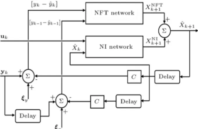
NFT are their corresponding weight and bias parameters. The architecture for the proposed observer is shown in Figure 1.
The training procedures of the NI and NFT, which are done o-line, are quite dierent. First, the NI is trained by the well-known backpropagation (BP) algorithm and, then, using the trained NI, the NFT is trained, based on the Backpropagation Through Time (BTT) algorithm. Detailed descriptions of training procedures are addressed in the next section.
OFF-LINE TRAINING FOR THENEURAL
OBSERVER
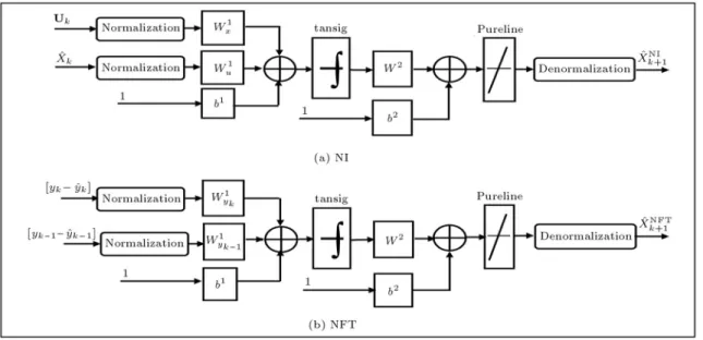
Both the NI and NFT are two-layer tansig/pureline MLP networks, as shown in Figure 2. Such MLP networks are universal approximators, because they
Figure1. Neural observer architecture.
can learn any nonlinear complex mapping using gener-ated input/target sets, given sucient neurons in the hidden layer 9]. Training procedures of the mentioned networks are, as follows, in the next subsections. BP Training forthe NI
The function of the NI is to identify the plant model (Equation 1) and to be used as a part of the observation process. It is also used to backpropagate the equivalent error to the NFT by calculating the plant Jacobians.
By using the state space model of the system, the problem of NI training can be regarded as an approx-imation process of state space nonlinear mapping, so that the NI can approximate the discrete-time model of the system as:
x NI
k+1 = NI ;
xMkukW NI
(12)
wherexMk is the state vector generated by the dieren-tial equations of the system (Equation 1) and x
NI
k+1 is the NI output vector.
As previously mentioned (in Figure 1), x NI
k+1 is the contribution of the NI network in the observed state vector (^xk
+1). Here, the training of the NI is to adjust its weight parameters so that it emulates the dierential Equation 1. The objective of training is to reduce average error dened by:
J= 12Nd Nd X
i=1
Nh;1 X
k=0 ;
xMk +1(i)
;x NI
k+1(i) T;
xMk +1(i)
;x NI
k+1(i)
(13) where Nd is the number of training sets, i represents the data set, which is the ith training sample andNh is the number of time horizons. Input-state training patterns are obtained from the operation history of the plant under various conditions.
One of the most important problems in observer operation is the measurement noise. Even if a typical observer can work in the presence of measurement noise, these noises are transferred to the estimated states and, sometimes, the performance of the observer deteriorates signicantly. One of the solutions to this problem, which is proposed in this paper, is to use neural network learning capabilities, in the same way that one can learn the neural observer, so that it cancels incoming noises from the outgoing states. For this reason, in the o-line training phase, the incoming states to the NI, i.e. xMk, are corrupted with a Gaussian white noise, while the noise-free states are used for error backpropagating. Using the proposed method, the neural network learns to cancel the noises, which are coming from the measurement channels. The same procedure would be employed in NFT training, as will be discussed. The block diagram for NI training is given in Figure 3.
Figure2. MLP network structure for (a) NI and (b) NFT.
Figure3. Block diagram for training the NI network. Using the backpropagation algorithm, the weight parameters of the NI are updated in the following manner:
Wk =Wk
;1+( ;1)
@J @Wk
(14)
whereand are learning rate and momentum coef-cient, respectively and should satisfy the following condition:
01: (15)
Through the learning process, and should be identied adaptively and normalization of training sets should be done. For more details of the BP method, readers are referred to 22].
The training would be terminated when the aver-age error between the plant states and NI outputs (J in Equation 13) converges to a small value.
The problem arising here is that, in a real time process,xMk does not exist to be fedback to the NI net-work, therefore, after the training is done, the following relation is used as an approximation to Equation 12 in
real time: ^ xk
+1= NI(^
xkukW
NI): (16)
BTT Training forthe NFT
As the observer structure (Figure 1 and Equation 11) indicates, the contribution of the NFT (Neural-Feedback-Tuning) is to close the estimation loop, be-cause the NI network is an open loop estimator and is not stable by itself. Here, the NFT makes the neural observer be a stable closed-loop estimator. As previously mentioned (Figure 2), the NFT network is a two-layer MLP, which has a universal approximation property. For NFT o-line training, a method, based on the Backpropagation-Through-Time (BTT) algo-rithm, is developed. The objective of this method is to minimize the following receding horizon cost function:
J = 12N+1 X
k=1
xMk ;x^k T
Q xMk ;^xk
(17)
where N is an appropriate time horizon and Q is a positive denite weighting matrix. The BTT algorithm can be regarded as a trial and error learning procedure, which consists of two main parts. First, from randomly selected initial states and an arbitrary given control eort (which can be randomly selected or generated by a designed control system), the plant model and observer are derived forN steps. Second, the weight and bias parameters in the NFT are updated, using the equivalent error generated. To perform these steps, the state sensitivity of the cost function is dened by:
kx,; @J @x^k
Using the chain rule, the above gradient can be devel-oped as:
kx=Q ;
xMk;x^k
+
@x^k +1 @x^k
T k +1 x + @x^k
+2 @x^k
T
k+2
x k= 12N;1 (19)
Nx =Q ;
xMN;x^N
+
@x^N +1 @x^N
T N
+1
x (20)
N+1
x =Q; xMN
+1 ;x^N
+1
: (21)
Using the weight parameters of the NI and NFT, the existing Jacobians can be expressed as:
@^xk +1 @x^k
=
@NI(^xkukW NI) @x^k
; "
@NFT; ^ ey
k^ ey
k ;1 W
NFT @^ey
k
#
C (22) @^xk
+1 @^xk
;1 =;
"
@NFT; ^ ey
k^ ey
k ;1 W
NFT @e^y
k ;1 # C (23) ^ ey k=
yk;Cx^k: (24)
The formula for derivation of MLP Jacobians@ NI
@^x k
@NFT
@^e y
k
and @NFT
@^e y
k ;1
is described in the Appendix, Equations A1 and A2.
Now, the o-line BTT training procedure of the NFT can be summarized as follows:
i) Generate small random weights and biases for the NFT network
ii) Set the plant initial states with random numbers in the operation region of the plant and observer initial states with arbitrary numbers (for example, zero)
iii) Forward pass: Run the plant model, neural ob-server and controller for N steps forward from k = 1 to N + 1. If there is not a designed control algorithm, set the control inputs as a sinusoidal function with random amplitude and frequency in the operation region of the plant. The forward pass generates sequences of plant states, xM
1 xM
2
xMN
+1 and observed states, ^
x1x^2 x^N
+1
iv) Backward pass: Using the operation results in Step (iii), run the state sensitivity equations backward from k = N + 1 to 1, to evaluate the equivalent error,kxk=N+ 1N1
v) Update the weights and biases of the NFT network using:
W
NFT(j+ 1) =j W
NFT(j) +j(j;1)
N
X
k=1
@x^k +1 @W
NFT(j) T
k +1
X (25)
where: @x^k
+1 @W
NFT(j) =
@NFT; ^ ey
k^ ey
k ;1 W
NFT(j) @W
NFT(j) +
@x^k
+1 @x^k
@^xk @W
NFT(j) +
@^xk
+1 @x^k
;1
@x^k ;1 @W
NFT(j)
: (26) j and j are momentum coecient and variable learning rate, respectively, and should be selected adaptively 22]. The terms @x^
k +1
@^x k and
@x^ k +1
@^x
k ;1 can be calculated using Equations 22 and 23
vi) Go to Step iii until convergence.
The training would be terminated when, by updating the NFT weights, no appreciable change in the receding horizon cost function (Equation 17) is observed.
In Equation 26, the formulas for derivation of @NFT(^e
y k
^ ey
k ;1W NFT(j))
@WNFT
(j) , which is the gradient of the MLP output with respect to its weights and biases vector, are explained in the Appendix, Equations A3 through A7.
To achieve the generalization property, the train-ing algorithm should be repeated for other sets of initial conditions and set-points iteratively. An important matter is the o-line training of NFT. In the forward pass phase, the output signals are corrupted with a Gaussian white noise but, in performance measure and state sensitivity equations, noise free output signals are backpropagated. Using this procedure, the NFT learns the noise cancellation property (the same as the NI, as described in the last section).
ADDITIVE ON-LINE ADAPTING PART In the previous section, a comprehensive neural ob-server was designed, based on the assumption that the mathematical model of the system is known and there are not catastrophic errors in the model. But, there are many nonlinear systems, in which the mathematical models are not completely known and/or some of their parameters are not certain. Although the neural observers, generally, have robustness properties, in the presence of large model errors, the observer results may
be unsatisfactory. One of the possible solutions to this problem is to add an adaptive online term, whose contribution is to compensate the remainder estimation error, due to unmodeled dynamics and/or parameter variations, from instantaneous output error feedback (measured output minus observed output).
In this paper, Linearly Parameterized Neural Networks (LPNNs) are used as the adaptive part. These networks are mathematically very simple and computationally ecient for on-line training. The neu-ral observer structure (Equation 11) can be modied by adding the on-line updating LPNN, as:
^ xk
+1=NI(^
xkukW NI) + NFT(yk;y^k]yk
;1 ;y^k
;1] W
NFT) + WB(yk;^yk) +bB]: (27) During real time implementation, the o-line trained parts (i.e., NI and NFT) are only simulated and are not updated, but, WB and bB are updated, at each time step, using the following recursive steepest descent algorithm:
Wkb =W
k;1
b +(;1) @Jk
@Wkb
(28)
where and are learning rate and momentum coecient, respectively, and Wb is a vector made by arranging the elements ofWB andbB.
The instantaneous performance measure (Jk) is dened by:
Jk = 12 (yk;y^k)
T(
yk;y^k): (29) Finally, @Jk
@Wk b
can be developed as: @Jk
@Wkb
= (^yk;yk)
TC @^xk @Wkb
(30)
where @x^ k
@Wk b
is calculated through the following recur-sive relation:
@^xk @Wkb
=
h
D1]D2]
Dn]I] i
n(nm+n) +
@NI(^xk ;1
uk ;1
W NI) @^xk
;1 ;
@NFT; ^ ey
k ;1^ ey
k ;2 W
NFT @e^y
k ;1 +WB
! C
! @^xk
;1 @Wkb
!!
: (31)
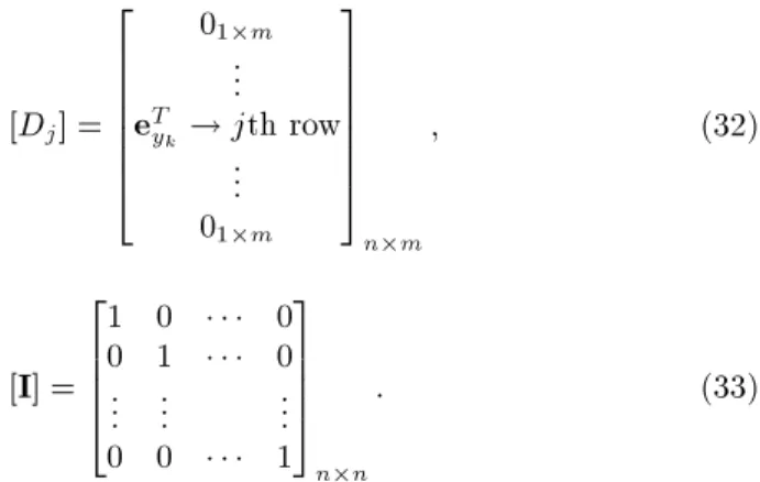
nandmhave been dened in the previous section and: Dj] =
2 6 6 6 6 6 6 4
01m ... eTy
k
!jth row ... 01m
3 7 7 7 7 7 7 5
nm
(32)
I] = 2 6 6 6 4
1 0 0
0 1 0
... ... ...
0 0 1
3 7 7 7 5
nn
: (33)
The training would be terminated when the instan-taneous performance measure (Equation 29) becomes less than a desired value or processor computation time becomes more than a time step. The archi-tecture of the overall neural observer is shown in Figure 4.
It is also noted that the stability of the on-line training part is not a challenging matter here, because the NI + NFT can stably observe the states, even though the on-line part is removed in the estimation process. The main role of the on-line part is not to stabilize the process, but to reduce the remainder error due to unmodeled dynamics. Most of the referred papers have used the on-line part as the process stabilizer 14-16], in which the guaranty of stability is crucial. Therefore, if the on-line updating (LPNN) tends to diverge in a time step, the algorithm will remove it in that step and, then, in the next step, on-line updating begins with zero (or random) initial weights and biases.
SIMULATION RESULTS
In this section, simulation results of two examples, illustrating the applicability of the proposed neural observer, are presented.
Case Study 1
Consider the Van der Pol oscillator 15] with the output subjected to the measurement noises:
_ x1=x2
_ x2=(1
;x 2 1)x
2 ;x
1 y=x1+y
ICs:x1(0) = 2 x2(0) = 1:
First, it is assumed that the model is perfect and is known and equal to 1.50. Initial conditions for the observer and time step are chosen as 15]:
^
x1(0) = ^x2(0) = 0 h= 0:3sec]:
Measurement noise, (y), is assumed to be white noise, with a variance equal to 0.1. The number of hidden neurons in the NI and NFT networks is selected to be 20 and 16, respectively.
First, NI and then NFT were trained o-line using BP and BTT, respectively. For o-line training, a hundred ICs were picked up randomly from the operating range of the plant. The training iteration was stopped when no appreciable change in the criterion function was observed. In this case, the observer results for an IC, which has not been used in the trainings, are reported in Figure 5. It is noted that, in this case, the on-line part is not presented. The results show that the proposed scheme yielded satisfactory smooth state estimates.
Second, it is assumed that the 's value are not known and, also, an unmodeled dynamics L(t) is added, such that:
_ x1=x2
_ x2=(1
;x 2 1)x
2 ;x
1+L(t):
For o-line training, the value of is chosen equal to 1.5, but, its real value (for the plant) is taken as 2.5. Initial conditions, measurement noise and time step are the same as the rst part. L(t) is selected to be a Gaussian white noise with the variance equal to 0.4. In this case, the behavior of the overall neural observer, in the presence of the on-line adapting part, is shown in
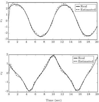
Figure 5. Real and estimated states of the Van der Pol
oscillator with noise.
Figure 6. Real and estimated states of the Van der Pol
oscillator with modeling error and noise.
Figure 6. By studying the results, it is obvious that the observation is quite satisfactory, even in the presence of a 40%parameter error ('s error) and almost large, unmodeled dynamics. In comparison to 15], where the observed states are noisy, due to measurement noise, the results of the proposed simulation show that the measurement noise is not transferred to the observed states.
Case Study 2
Consider a single-link robot manipulator, rotating in a vertical plane 14], described as:
_ x1
_ x2
=
x2 ;sin(x
1) +u(t)
+ f y=x1+y
where the unmodeled dynamics are given as follows: f = 0:01
x1cos(x1) x2sin(x2)
and u(t) is selected to be zero. In addition to what has been considered in 14], this paper considers unmodeled dynamics, f, and measurement noise,y, which introduces a more general case. After o-line training, the overall observer was tested with plant initial conditions as follows:
x1(0) = 2 x2(0) = 1:
While the observer initial conditions, time step and measurement noise are chosen as:
^
x1(0) = ^x2(0) = 0 h= 0:4sec]
y ! white noise, with the variance equal to 0.15 the number of hidden neurons in the NI and NFT networks is selected as 23 and 18, respectively. The
Figure7. Real and estimated states of the robot
manipulator with modeling error and noise.
behavior of the overall neural observer is shown in Figure 7. The results are completely satisfactory, even in the presence of measurement noise and unmod-eled dynamics. The results verify, again, that the observed states are not noisy, due to measurement noise.
CONCLUSION
In this paper, a new neural observer is designed and it is shown that it can provide a good enough estimation process for nonlinear dynamic systems in the presence of internal uncertainties and external perturbations. The proposed scheme consists of three neural parts, two of which are o-line trained MLP networks and the other being an on-line updating LPNN. If the mathematical model is perfect, the o-line parts are sucient for the observation process, but, in the presence of model error, the on-line part adapts and compensates the estimation error, due to model error. By adding a time delay term, the arising dierential eects are compensated. MLP's o-line training, using noise corrupted data sets, helps the observer to cancel most of the measurement noises from the observed states. The numerical experiments demonstrate the high eectiveness of the proposed technique.
REFERENCES
1. Luenberger, D.G. \Observing the state of linear sys-tems",IEEE Transactions on Military Electron,8, pp
74-90 (1964).
2. Gauthier, J.P., Hammouri H. and Othman S. \A simple observer for nonlinear systems: Applications to bioreactors", IEEE Transactions on Automatic Con-trol,37, pp 875-880 (1992).
3. Marino, R. and Tomei, P. \Adaptive observer with arbitrary exponential rate of convergence for nonlinear systems", IEEE Transactions on Automatic Control,
40, pp 1300-1304 (1995).
4. Ciccarella, G., Dalla Mora, M. and Germani, A. \A Luenberger-like observer for nonlinear systems", In-ternational Journal of Control,45, pp 537-556 (1993).
5. Walcott, B.L., Corless, M.J. and Zak, S.H. \Compara-tive study of nonlinear state observation technique",
International Journal of Control, 45, pp 2109-2132
(1987).
6. Tsinias, J. \Further results on observer design prob-lem", Systems and Control Letters, 14, pp 411-418
(1990).
7. Sira-Ramirez, H. and Spurgeon, S.k. \On the robust design of sliding observers for linear systems",Systems and Control Letters,23, pp 9-14 (1994).
8. Funahashi, K. and Nakamura, Y. \Approximation of dynamic systems by continuous time recurrent neural networks",Neural Networks,6, pp 801-806 (1993).
9. Hornik, K., Stinchcombe, M. and White, H. \MLP's are universal approximators",Neural Networks,2, pp
359-366 (1989).
10. Narendra, K.S. and Parthasarathy, K. \Identication and control of dynamic systems using neural net-works",IEEE Transactions on Neural Networks,1, pp
4-27 (1990).
11. Zhu, R., Chai, T. and Shao, C. \Robust nonlinear adaptive observer design using dynamic recurrent neu-ral networks",Proc. Amer. Cont. Conf., pp 1096-1100, New Mexico (June 1997).
12. Wang, J. and Wu, G. \Real time synthesis of linear state observers using a multilayer recurrent neural networks",Proc. IEEE Int. Conf. Industrial Tech., pp 287-282 (1994).
13. Ahmed, M.S. and Riyaz, S.H. \Design of dynamic neural observers", IEEE Proc. Cont. Theory Appl.,
147(3), pp 257-266 (May 2000).
14. Vargas, J.R. and Hemerly, E.M. \Adaptive observers for unknown general nonlinear systems",IEEE Trans-actions on Systems, Man. and Cybernetics,31(5), pp
683-690 (2001).
15. Poznyak, A. and Yu, W. \Robust asymptotic neuro-observer with time delay term",International Journal of Robust and Nonlinear Control, 10, pp 535-559
(2000).
16. Sun, F., Sun, Z. and Woo, P. \Neural network-based adaptive controller design of robotic manipulators with an observer",IEEE Transactions on Neural Networks,
12(1), pp 54-67 (2001).
17. Morino, P., Milano, M. and Vasca, F. \Linear quadratic state feedback and robust neural network estimator for eld-oriented-controlled induction mo-tors", IEEE Transactions on Industrial Electronics,
46(1), pp 150-161 (1999).
18. Pilluta, S. and Keyhani, A. \Development and im-plementation of neural network observers to estimate the state vector of a synchronous generator from online operating data",IEEE Transactions on Energy Conversion,14(4), pp 1081-1087 (1999).
19. Powell, J.D., Fekete, N.P. and Chang, C.F. \Observer-based air-fuel ratio control", IEEE Control Systems Magazine,18(5), pp 72-83 (1998).
20. Webros, P.J. \Backpropagation through time: What it does and how to do it",Proc. IEEE,78, pp 1550-1560
(Oct. 1990).
21. Park, Y.M., Choi, M.S. and Lee, K.Y. \An optimal tracking neuro-controller for nonlinear dynamic sys-tems", IEEE Transactions on Neural Networks, 7(5),
pp 1099-1110 (1996).
22. Hagan, M.T., Demuth, H.B. and Baal, M., Neural Network Design, PWS Publications (1996).
APPENDIX
Derivation ofMLP Jacobian
Suppose there exists a two-layer tansig/pureline MLP network where its input and output arepn1andam1, respectively. The MLP Jacobian is given by:
da dp
=diag(a(j))]m m
W 2 diag;
1;tansig(n 1(j))]
2
s1 s
1 W
1
diag
1 p(j)
nn
(A1)
whereW1W2b1andb2are the weights and biases for the rst and second layers, respectively, and a and pare expressed as:
p=
8 > > > < > > > :
max(p(1));min (p(1)) max(p(2));min (p(2))
...
max(p(n));min (p(n)) 9 > > > = > > >
n1
a=
8 > > > < > > > :
max(a(1));min(a(1)) max(a(2));min(a(2))
...
max(a(m));min(a(m)) 9 > > > = > > >
m1
(A2)
Gradient ofMLP Output with Respect to its Weightsand Biases
This gradient can be expressed as: @a
@W =12diag( a)]s2
s 2
"
@n 2 @W 1
@n 2 @b
1
@n 2 @W 2
@n 2 @b
2
#
s2 (ns
1 +s
1 +s
2 s
1 +s
2 )
(A3) where W is a vector made by arranging the elements ofW1W2b1andb2and one has:
s2=m
@n
2 @b
2
= 2 6 6 6 4
1 0 0
0 1 0
... ... ...
0 0 1
3 7 7 7 5
S2 S
2
" @n
2 @W 2
# =
"
@n 2 @W
2(1)
S2 S
1
@n 2 @W
2(2)
S2 S
1
@n
2 @W
2(S2)
S2 S
1 #
S2 (S
2 S
1 )
(A4)
@n
2 @W
2(j)
= 2 6 6 6 6 6 6 4
0 1S
1 ... aT
1 !j
th row ... 0
1S 1
3 7 7 7 7 7 7 5
S2 S
1
(A5)
" @n
2 @b
1 #
=W
2 h
diag
1;tansig(n 1(j))]
2 i
S1 S
1 (A6)
@n
2 @W 1
S2 (S
1 n)
=W 2
" diag
1;tansig (n
1(j))] 2
#
S1 S
1
@n 1 @W 1
@n 1 @W 1
=
"
@n 1 @W
1(1)
S1 n
@n
1 @W
1(2)
S1 n
@n
1 @W
1(S1)
S1 n
#
S1 (S
1 n)
@n
1 @W
1(j)
= 2 6 6 6 6 6 6 4
0 1n
... pT !j
th row ... 0
1n 3 7 7 7 7 7 7 5
S1 n