A&A 570, A20 (2014)
DOI:10.1051/0004-6361/201423831 c
ESO 2014
Astronomy
&
Astrophysics
A connected component-based method for efficiently integrating
multi-scale
N-body systems
Jürgen Jänes
1,, Inti Pelupessy
2, and Simon Portegies Zwart
21 Faculty of Science, University of Amsterdam, PO Box 94216, 1090 GE, Amsterdam, The Netherlands 2 Leiden Observatory, Leiden University, PO Box 9513, 2300 RA, Leiden, The Netherlands
e-mail:[email protected]
Received 18 March 2014/Accepted 20 July 2014
ABSTRACT
We present a novel method for efficient direct integration of gravitationalN-body systems with a large variation in characteristic time scales. The method is based on a recursive and adaptive partitioning of the system based on the connected components of the graph generated by the particle distribution combined with an interaction-specific time step criterion. It uses an explicit and approximately time-symmetric time step criterion, and conserves linear and angular momentum to machine precision. In numerical tests on astrophysically relevant setups, the method compares favourably to both alternative Hamiltonian-splitting integrators as well as recently developed block time step-based GPU-accelerated Hermite codes. Our reference implementation is incorporated in the HUAYNO code, which is freely available as a part of the AMUSE framework.
Key words.methods: numerical – stars: kinematics and dynamics – gravitation
1. Introduction
Direct integration of the classicalN-body problem is an impor-tant tool for studying astrophysical systems. Examples include planetary systems, open and globular clusters dynamics, large-scale dynamics of galaxies, and structure formation in the uni-verse. In many cases the calculations involve systems where the intensity of gravitational interactions spans multiple orders of magnitude with corresponding time scale variations. For exam-ple, the initial stages of cluster formation are now thought to resemble multi-scale fractal structures (Goodwin & Whitworth 2004), and stellar systems are invariably formed with a high frac-tion of binaries and hierarchical multiples that affect the dynam-ical evolution in crucial ways (Portegies Zwart et al. 2010).
In practice, integrating multi-scale systems requires spe-cialised methods that vary the resolution at which we treat diff er-ent parts of the simulation. The aim of this is to obtain a solution with an acceptable accuracy without unnecessarily spending computational resources on the slowly evolving parts of the sim-ulation. In generic N-body integrators, this idea is most com-monly implemented viaparticle-based block time steps– every particle in the system maintains an individual time step limited to discrete values in a power of two hierarchy. These block time steps are then typically used to determine the frequency of cal-culating the total force acting on a particle (e.g.McMillan 1986; Makino 1991;Konstantinidis & Kokkotas 2010).
While considerably speeding up calculations, particle-based block time steps are nevertheless limited in their ability to treat the extreme scale differences often present inN-body systems. Hence, complementary strategies, such as binary regularisa-tion and neighbourhood schemes, have been devised. These ap-proaches complicate the implementation ofN-body integrators,
Current address: the Gurdon Institute and Department of Genetics,
University of Cambridge, Cambridge CB3 0DH, UK
and often introduce new method-specific free parameters. It is also unclear whether these combinations of multiple strategies represent the best possible approach for integrating multi-scale N-body systems. These issues provide a clear incentive to ex-plore alternative methods.
InPelupessy et al.(2012), we derived genericN-body inte-grators that recursively and adaptively split the Hamiltonian of the system. These methods show improved conservation of the integrals of motion by always evaluating partial forces between particles in different time-step bins symmetrically, and by using an approximately time-symmetric time-step criterion.
In the present work, we introduce a new Hamiltonian-splitting integration method that is particularly adept at integrat-ing initial conditions with significant hierarchical substructure. Our approach is based on assigning time steps to individual interactions, followed by partitioning the system Hamiltonian based on a graph formed by the set of interactions that are faster than a fixed threshold time step. The successive partition-ing produces closed Hamiltonians such that we can easily use specialised solvers for situations where more efficient solvers are available. Numerical experiments show that our integrator compares favourably to existing splitting methods even for an ordinary Plummer sphere where the prevalence of isolated sub-systems is not immediately obvious. For astrophysically realis-tic systems explicitly chosen for their multi-scale substructure, the performance gains increase can be orders of magnitude. An implementation of the method is incorporated in the HUAYNO code, which is freely available as a part of the AMUSE frame-work (Portegies Zwart et al. 2013;Pelupessy et al. 2013) and which was used for the tests presented in this paper.
Our method is similar in spirit, and accelerates the calcu-lation of the N-body problem for much the same reasons as the well known neighbour schemes. The main idea is to di-vide the total force acting on a particle into a fast and a slow
component based the distance to the given particle. Different ap-proaches have been used for treating fast and slow components. The Ahmad-Cohen neighbourhood scheme (Ahmad & Cohen 1973) treats fast components with a more strict time step criteria. Alternatively, the PPPT scheme (Oshino et al. 2011) integrates fast components with a fourth-order Hermite method while using a leapfrog-based tree code for the long range interactions. The criteria for determining neighbourhood memberships are heuris-tics known to work in numerical experiments, e.g. a sphere with a fixed radius centred on the acting particle. These methods need to continuously update neighbourhood memberships as the sys-tem state changes throughout the simulation. In addition, neigh-bourhood schemes only make a single distinction between treat-ing small subsystems such as hard binaries or many-body close encounters, and the large scale dynamics. It is difficult to gener-alise a neighbourhood scheme beyond a binary differentiation of the particle distribution.
In Sect. 2 we describe a bottleneck in existing general N-body splitting methods, and derive our novel splitting scheme that overcomes this bottleneck. Section3presents the results of numerical tests comparing of our method to existing approaches. Finally, in Sect.4we discuss possible improvements and exten-sions to our work, including the feasibility of integrating general N-body systems using purely interaction-specific time steps.
2. Method
2.1. Deriving time stepping schemes via Hamiltonian splitting
The Hamiltonian for a system ofN particlesi = 1. . .N under gravitational interaction can be represented as a sum of momen-tum termsTiand potential termsVi j:
H(pi,qi)=T +V = N
i=1
Ti+ N
i,j=1 i<j
Vi j (1)
Ti=
pi 2
2mi
(2)
Vi j=−G
mimj
q2 i j+ε2
(3)
wheremi is the mass, qi is the position and pi is the
momen-tum of theith particle of the system, andqi j = qi−qj. The
evolution of the state of the system for a time steph is given formally by the flow operatorEH(h)=exp(hH) whereHis the
Hamiltonian vector field corresponding toH.
If the HamiltonianHof the system is representable as a sum of two sub-Hamiltonians,H = A+B, we can approximate the time evolution underHwith a sequence of time evolution steps under the sub-HamiltoniansAandB. A straightforward succes-sive application of the time evolution underAfollowed by the time evolution underBgives a first-order approximation of the full time evolution underA+B, while a second-order accurate ap-proximation can be obtained with one additional operator eval-uation (Sanz-Serna & Calvo 1994, Sect. 12.4; alsoHairer et al. 2006).
EA+B(h)=EA(h/2)EB(h)EA(h/2)+O
h2. (4)
The sub-HamiltonianAis evolved in two steps ofh/2 and the sub-HamiltonianB is evolved in a single step h. We can take advantage of this property of the splitting formula by dividing
terms associated with fast interactions intoAand terms associ-ated with slow interactions intoB. We can proceed by applying this splitting procedure to different sub-Hamiltonians multiple times, thereby constructing an integrator that evaluates parts of the Hamiltonian ath,h/2,h/4 etc., similarly to the power of two hierarchy used in block time step schemes. This approach was followed inPelupessy et al.(2012), below we introduce some notation and give a rough derivation of the integrators there.
Hamiltonians consisting of a single momentum term and Hamiltonians consisting of a single potential term have analytic solutions. For a momentum term of theith particle
Hi(pi,qi)=Ti=
pi,pi
2mi
(5) the solution consists of updating the position of theith particle under the assumption of constant velocity for a time period ofh (all positions except the position of theith particle and the mo-menta of all particles remain unchanged).
qi(t+h)=qi(t)+hui(t). (6)
We call the time evolution operator for the momentum term of theith particle thedrift operatorand writeDh,Ti.
For a single potential term between particlesiand j Hi j(pi,qi)=Vi j=−G
mimj
q2i j+ε2
(7)
the solution consists of updating the momenta of theith and jth particles under the assumption of constant force for a time period of h (all momenta except the momenta of the ith and jth particles and the positions of all particles remain unchanged).
pi(t+h)= pi(t)+hFi j(t) (8)
pj(t+h)= pj(t)+hFji(t). (9)
We call the time evolution operator for the potential term be-tween theith and jth particles the kick operator and writeKh,Vi j.
In addition to the kick and drift operators, the two-body Hamiltonian
Hi j(pi,qi)=Ti+Tj+Vi j=
pi,pi
2mi +
pj,pj
2mj −
Gmimj q2
i j+ε2
(10)
is solved (semi-) analytically by the Kepler solution1.
InPelupessy et al.(2012), we derive multiple integrators that recursively and adaptively split the system Hamiltonian through the second-order splitting formula (4). At every step in the re-cursion, all particles under consideration are divided into a slow setS and a fast setF by comparing the particle-specific time step functionτ(i) to a pivot time steph.
S ={i∈1. . .N:τ(i)≥h} (11) F ={i∈1. . .N:τ(i)<h}. (12) Using the two sets S and F, we can rewrite the system Hamiltonian as follows.
H =HS+HF+VS F. (13)
The sub-Hamiltonian HS can be thought of as a “closed
drifts of particles inS and all kicks where both participating par-ticles are inS.The same property holds for the sub-Hamiltonian HFand the particles inF. The mixed termVS Fcontains all kicks
where one particle is inS and the other is inF.
We proceed by applying the second-order splitting rule (4): Eh,H =Eh,HS+HF+VS F (14)
≈Eh/2,HFEh,HS+VS FEh/2,HF (15)
(this is not the only conceivable approximation). The sub-Hamiltonian HF is closed, and consists of particles where
τ(i)<h. We integrate HF by recursively applying the entire
“slow/fast” partitioning, but using a smaller pivoth/2. In con-trast, bothHS = TS +VS andVS F are explicitly decomposed
into individual kicks and drifts which are applied using the cur-rent pivot time steph. We refer to this particular choice as the HOLD method (since it “holds”VS F for evaluation at the slow
timestep).
Eh,HS+VS F =Eh,TS+VS+VS F (16)
≈Dh/2,TSKh,VS+VS FDh/2,TS. (17)
The pivot time stephis halved with each consecutive partition-ing, and the recursion terminates when all remaining particles are placed into theS set.
As noted previously, recursively and adaptively splitting the system Hamiltonian using the second order splitting rule (Eq. (4)) is similar to conventional block time steps. Both approaches evolve different parts of the system using time steps that belong to a power of two hierarchy. However, the Hamiltonian splitting method derived above evaluates pairwise particle forces symmetrically in the sense that a “kick” from par-ticlei to particle j(Eq. (8)) is always paired with an opposite kick from particlejto particlei(Eq. (9)). Furthermore, the kicks acting upon a particle at any given timestep typically correspond to partial forces only. This is in contrast to conventional block time steps where we always calculate thetotalforce acting on a particle at the frequency determined by the particle-specific time step criteriaτ(i)
pi(t+h)= pi(t)+h N
j=1,ji
Fi j(t) (18)
where, Fi j(t) is the force acting on particleidue to particle j, derived from extrapolated positions if necessary. Specifically, in situations where the position of particlejhas not been calculated for timet, we calculate the force by extrapolating the position attfrom the last known position. This can happen when parti-cleiis assigned a smaller time step than particle j. We refer to this method as BLOCK, and include it as a reference in our nu-merical tests to determine whether more “aggressive” splitting methods (such as HOLD) reduce the number of kicks and drifts while maintaining the accuracy of the solution.
The HOLD method evolves all kicks between fast particles at the fast time step. This is inefficient in the presence of iso-lated fast subsystems, as interactions between particles that be-long to different subsystems could be evolved at a slower time step. As an extreme example, consider a Plummer sphere with each star being replaced by a stable hard binary. Here, every star has a close binary interaction that needs to be evaluated at a fast time step. However, the HOLD integrator will in this case inte-grate all interactions, including long-range interactions between stars in different binaries at a time step determined the binary in-teractions. The behaviour of the method becomes equivalent to evolving the entire system with a shared global time step!
In addition to the dramatic example just discussed, the same inefficiency – evaluating long-range interactions between iso-lated fast subsystems at time steps determined by fast inter-actions inside the subsystems – can manifest itself in other situations, such as the following.
– In a system with multiple globular clusters, each individual globular cluster is a subsystem.
– In a globular cluster with planets around some of the stars, each star with planets is a subsystem.
– In a single globular cluster, each close encounter between two or more stars is a subsystem.
2.2. Hamiltonian splitting with connected components
The partitioning used in the HOLD method is based on a particle-specific time step criteria τ(i), which by defini-tion cannot separate slow and fast interacdefini-tions in situadefini-tions where all particle-specific time steps have the same (fast) value. We therefore introduce theinteraction-specifictime step criterionτ(i,j)
τ(i,j)=ηmin ⎛ ⎜⎜⎜⎜⎜
⎜⎜⎝ τfreefall(i,j) 1−1
2
dτfreefall(i,j)
dt
, τflyby(i,j)
1−12dτflyby(i,j)
dt
⎞ ⎟⎟⎟⎟⎟
⎟⎟⎠ (19)
whereτfreefall(i,j) and τflyby(i,j) are proportional to the inter-particle free-fall and interinter-particle flyby times as defined by Eqs. (13) and (16) inPelupessy et al. (2012), andη is an ac-curacy parameter.
We split the system Hamiltonian using the connected com-ponents (Cormen et al. 2001, Sect. B.4) of the undirected graph generated by the time step criteriaτ(i,j). Specifically, the parti-cles of the system correspond to the vertices of the graph, and there is a edge between particlesiand jif their interaction can-not be evaluated at the threshold time steph.
τ(i,j)<h. (20)
Figure1we visualises the time step graphs at varying values of the pivot time stephfor three different fractal initial conditions with different fractal dimension (described further in Sect.3). As the pivot time stephdecreases, the set of interactions (and asso-ciated particles) that cannot be evaluated at the current pivot time step gradually decreases as well. Although for visualisation pur-poses, we plot the time step graph of the entire system for vary-ingh, the connected components (CC) splitting method we are about to introduce typically calculates CC for the entire system only once, at the largest pivot time step. At smaller pivot time steps, the connected components search is only calculated for parts of the system. The intuition behind this partitioning comes from clustering by maximising the margin between individual clusters as described inDuan et al.(2009).
Given a fixed pivot time step h, let the setsCi,i = 1. . .K
contain vertices ofKnon-trivial connected components, and the setR(“remainder set”) contain all particles in trivial connected components2. Based on the particle setsC
iandR, we rewrite the
Hamiltonian of the system in the following form
H=HC+HR+VCC+VCR (21)
Fig. 1.Time step graphs generated byτ(i,j) at different levels of the time step hierarchy (left to right) for three values (top to bottom rows) of the fractal dimension. We plot particles that have been passed on as a part of a connected component from the previous time step level as black, grey points indicate points that are inactive on a given level (because they formed a single or binary component at a lower level). Thin grey lines indicate interactions withτ(i,j)<h. Indicated in each frame are the fractal dimension (top left), and (on thebottom right) the level in the hierarchy, the number of connected components (cc) at this level, as well as the number of components that are single (s) and binary (b), and the total number of particles.
where the individual terms are defined as follows.
HC = K
i=1
HCi = K
i=1 ⎛ ⎜⎜⎜⎜⎜ ⎜⎜⎜⎜⎜ ⎜⎜⎝
j∈Ci
Tj+
j,k∈Ci i<j
Vjk
⎞ ⎟⎟⎟⎟⎟ ⎟⎟⎟⎟⎟
⎟⎟⎠ (22)
HR =TR+VR=
i∈R
Ti+
i,j∈R i<j
Vi j (23)
VCC = K
i,j=1 i<j
VCiCj = K
i,j=1 i<j
⎛ ⎜⎜⎜⎜⎜ ⎜⎜⎜⎜⎜ ⎜⎜⎝
k∈Ci l∈Cj
Vkl
⎞ ⎟⎟⎟⎟⎟ ⎟⎟⎟⎟⎟
⎟⎟⎠ (24)
VCR = K
i=1
VCiR= K
i=1 ⎛ ⎜⎜⎜⎜⎜ ⎜⎜⎜⎜⎜ ⎜⎝
j∈Ci k∈R
Vjk
⎞ ⎟⎟⎟⎟⎟ ⎟⎟⎟⎟⎟
evolve_cc(H, h):
// split_cc() decomposes particles in H (eq 25) into: // 1) K non-trivial connected components C_1..C_K // 2) Rest set R
(C_1..C_K, R) = split_cc(H, h)
// Independently integrate every C_i at reduced pivot time step h/2 (eq 27) for C_i in C_1..C_K:
evolve_cc(C_i, h/2)
// Apply drifts and kicks at current pivot time step h (eq 30) drift(R, h/2) // evolves T_R
kick(R, R, h) // evolves V_RR
kick(C_1..C_K, C_1..C_K, h) // evolves V_CC (eq 23) kick(C_1..C_K, R, h) // evolves V_CR (eq 24) drift(R, h/2) // evolves T_R
// Independently integrate every C_i at reduced pivot time step h/2 (eq 27) for C_i in C_1..C_K:
evolve_cc(C_i, h/2)
Fig. 2.Pseudocode for a second-order CC splitting routine for integrating a set of particlesHfor time steph.
The termHC is the sum of all closed Hamiltonians HCi, each
corresponding to one of theKconnected components. In every HCiall drifts and some kicks cannot be evolved at the time steph
without violating the time step criteria. The termHRconsists of
the closed Hamiltonian formed by all of the particles in the rest system. All drifts and kicks inHRcan be evolved at the current
time steph.
The termVCC contains all kicks between particles that are indifferent connected components. These kicks can be evalu-ated at the time steph. We point out thatVCCexplicitly contains the terms that are evolved inefficiently in the HOLD method. Similarly,VCRcontains all kicks where one of the particles is in a connected componentCi, and the other is in the rest setR.
We split the system HamiltonianHby applying the second-order splitting rule (4):
Eh,H =Eh,HC+HR+VCC+VCR (26) ≈Eh/2,HCEh,HR+VCC+VCREh/2,HC (27)
such that individual connected componentsCiare independently
evolved at a higher pivot time steph/2 via recursion.
Eh/2,HC = K
i=1
Eh/2,HCi. (28)
All remaining terms (includingVCC) are decomposed into indi-vidual drifts and kicks using the second-order splitting rule (4). Eh,HR+VCC+VCR =Eh,TR+VR+VCC+VCR (29)
≈Dh/2,TRKh,VR+VCC+VCRDh/2,TR (30)
=Dh/2,TRKh,VRKh,VCCKh,VCRDh/2,TR. (31)
As with the HOLD method, the pivot time steph is halved at each successive partitioning such that at some point, all remain-ing particles are in the remainder setR.
Finally, the partitioning can lead to situations whereHCi is
a two-body Hamiltonian (Eq. (10)). We can use this property by integrating these cases with a dedicated a Kepler solver (we discuss this further in Sect.3.2).
2.3. Implementation
We implemented the CC split in the HUAYNO code, which is freely available as a part of the AMUSE framework. Figure2 sketches the main routine of the CC integrator in pseudocode, including explicit references to the corresponding equations and variables used in the derivation of the method (Sect.2.2).
Subroutines and data structures that store the system state, calculate time steps, apply kicks and drifts to groups of parti-cles, and gather statistics, are shared with other integrators such as the HOLD method. All particle states are kept in a contiguous block of memory. The connected component algorithm is imple-mented as a breadth-first search. It reshuffles particle states such that particles in the same connected component or rest set are kept adjacent to each other. Connected components are repre-sented by a start and an end pointer to the contiguous array of particle states.
The time complexity of the connected component decompo-sition forNparticles has an upper bound ofO(N2). This matches the time complexity of the splitting step of the HOLD method – while the actual shuffling of the particles intoS andF sets is O(N), this division is based on the preceding step of calculating particle-based time stepsτ(i) for all particles, which isO(N2).
For the special case where all interactions between theN par-ticles are below the thresholdh, the complexity of the connected components decomposition isO(N). This can happen multiple times (at consecutive recursion levels) when the initial value of the pivot time step h is sufficiently large. Figuratively, if par-ticleX has a known connected component while particle Y is unassigned, we can assign particleY to the connected compo-nent of particleXbased on a single time step evaluationτ(X,Y). A key step of the connected components search is choosing a particleX with a known connected component, followed by assigning the membership of X to all unassigned particlesUk
whereτ(X,Uk)<h. For the special case under consideration, a
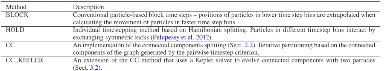
Table 1.Overview of the integrators used in the numerical tests.
Method Description
BLOCK Conventional particle-based block time steps – positions of particles in lower time step bins are extrapolated when calculating the movement of particles in faster time step bins.
HOLD Individual timestepping method based on Hamiltonian splitting. Particles in different timestep bins interact by exchanging symmetric kicks (Pelupessy et al. 2012).
CC An implementation of the connected components splitting (Sect.2.2). Iterative partitioning based on the connected components of the graph generated by the pairwise timestep criterion.
CC_KEPLER An extension of the CC method that uses a Kepler solver to evolve connected components with two particles (Sect.3.2).
Notes.The implementations share a significant amount of the code and data structures used for storing system state, calculating time steps, and evaluating (partial) forces.
Sect.3indicate that the reduction in time step evaluations does translate into improved performance.
3. Tests
We present results of numerical experiments of the CC split-ting method described in the previous section. We confirm that the CC method works as intended conceptually by comparing to alternative Hamiltonian splitting methods (see Table1for an overview). Specifically, we demonstrate that the connected com-ponents search does not use excessive computational resources, reduces the number of elementary operations (kick, drift and time step evaluations) while maintaining the accuracy of the solution, and performs particularly well on multi-scale prob-lems. Finally, we compare the CC method to establishedN-body codes. We useN-body units as described inHeggie & Mathieu (1986).
3.1. Smoothed Plummer sphere test
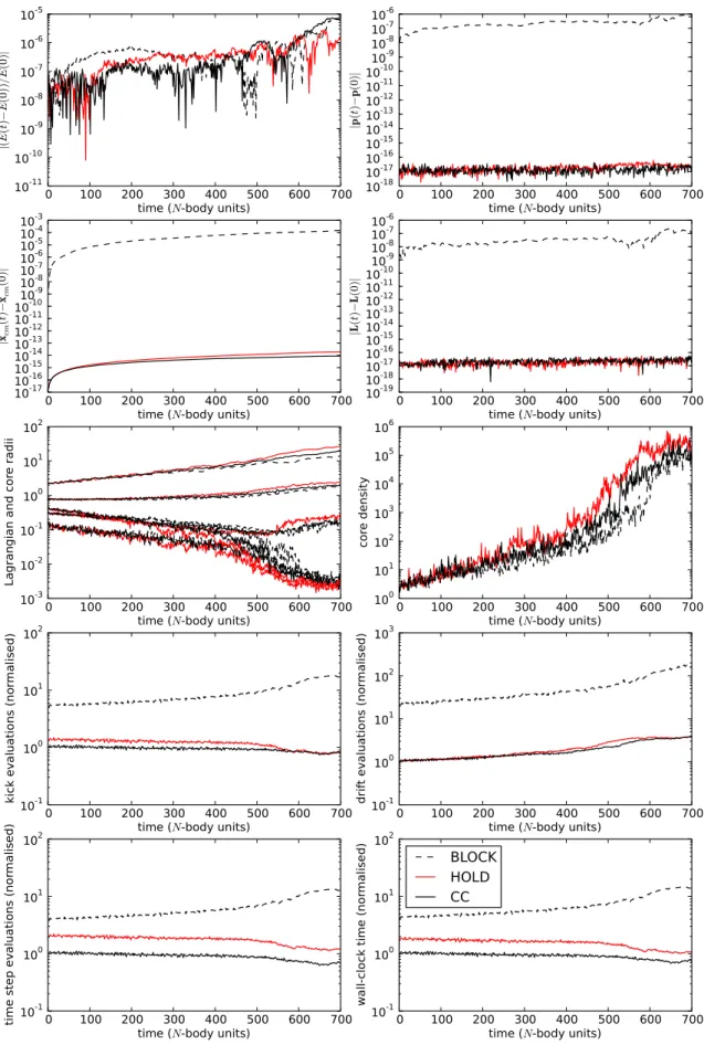
We begin by integrating an equal-mass 1024-body Plummer sphere with softening (ε = 1/256) for 700N-body time units using a time step accuracy parameter ofη = 0.01. We choose initial velocities such that the Plummer sphere is in a dynamic equilibrium. This setup is chosen to match the long-term inte-gration tests inNitadori & Makino(2008, their Sect. 3.2).
Figure3visualises the conservation of the integrals of mo-tion, the time evolution of the mass distribumo-tion, and perfor-mance metrics. While all three methods show similar energy conservation properties, only HOLD and CC maintain centre of mass, linear momentum and angular momentum near machine precision. As noted previously inPelupessy et al.(2012), this is caused by unsynchronised kicks which are only present in the BLOCK scheme. The solutions obtained by all three methods reproduce known results in terms of Lagrangian radii, the core radius and the core density. The CC scheme is about twice as fast than the HOLD scheme at the beginning of the simulation, and remains the fastest scheme throughout the run. The overall runtime measurements correlate with the number of time step formula evaluations and, to a lesser extent, the number of kick and drift formula evaluations. This indicates that the improved runtime is attributable to a reduction of time step, kick and drift formula evaluations.
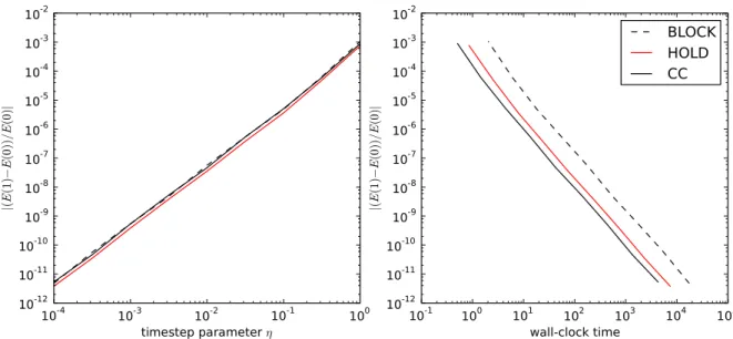
The left plot of Fig. 4 visualises energy error of evolving the softened Plummer sphere as described previously, but for 1N-body units and under varying time step accuracyη. As pre-dicted, all three methods show second order behaviour. On the corresponding wall-clock time vs energy error plot on the right
CC consistently outperforms HOLD, followed by BLOCK. We emphasise that the Plummer sphere is a spherically symmetric configuration with a smoothly changing mass distribution, and a non-zero softening lengthεsets an upper limit on the hardness of the binaries that can form during the simulation. Hence, we would not expect the CC scheme to have a significant advantage over the HOLD method.
3.2. Unsoftened Plummer sphere test
We proceed by evolving an equal-mass 1024-body Plummer sphere without softening through core collapse. We choose ini-tial velocities consistent with a dynamic equilibrium, as in the softened case considered previously. This setup is chosen to match a test used on a modern implementation of a fourth-order Hermite scheme with block time steps in Konstantinidis & Kokkotas(2010, their Sect. 3.4.1).
In addition to the HOLD and CC schemes that have been introduced previously, we also test a modification of the CC scheme with a dedicated Kepler solver (CC_KEPLER). In this scheme a Kepler solver is used for evolving connected compo-nents consisting of two particles. This is a form of algorithmic regularisation of binaries, but note that the regularisation follows naturally from the structure of the integrator and no separate bi-nary detection or additional free parameters are necessary. The implementation of the Kepler solver is based on a universal vari-able formulation (Bate et al. 1971).
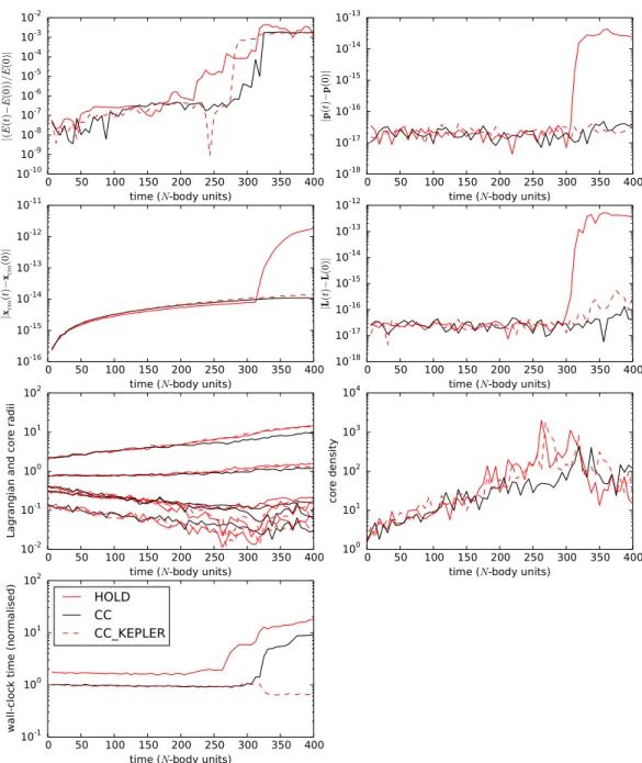
Results of the core collapse simulation are visualised in Fig.5. All three methods produce solutions that are realistic in terms of the evolution of the mass distribution. Energy conser-vation is comparable to what is observed in Konstantinidis & Kokkotas(2010). Other integrals of motion show conservation around machine precision with the exception of a jump in the HOLD method around core collapse (this is caused by a high speed particle escaping from the system, causing a loss of preci-sion in the force evaluations).
Before core collapse, execution times are roughly equiva-lent to the softened case considered previously (Sect.3.1) – CC shows a modest improvement over HOLD, and CC_KEPLER is very close to CC. Around core collapse, execution times of the HOLD and CC methods gradually increase by an order of mag-nitude (the CC method still consistently outperforms the HOLD method). In contrast, execution time used by the CC_KEPLER method remains relatively uniform throughout the simulation, including core collapse.
Fig. 4.Left: time step accuracy parameterηvs. energy error for integrating a 1024-body Plummer sphere for 1N-body units.Right: corresponding wall-clock time vs. energy error from the same set of tests.
(Gonçalves Ferrari et al. 2014). The main source of errors in Sakura comes from many-body close encounters, as these are difficult to decompose into two-body interactions. In contrast, CC_KEPLER only uses the binary solver for an isolated binary system, and switches to the regular many-body integrator when necessary (this is further discussed in Sect.4.1).
3.3. Fractal distributions
Since our new methods are based on the partitioning of the parti-cle distribution in connected subsystems, we expect the method to be especially well suited to situations where substructure with extreme density contrasts exist. We therefore proceed by inte-grating a set of initial conditions developed with the aim of describing a star cluster with fractal substructure (Goodwin & Whitworth 2004). These initial conditions mimic the observed distribution of young stellar associations. They are parametrized by a fractal dimension: a low fractal dimension leads to an in-homogeneous (“structured”) distribution of stars whereas a high fractal dimension leads to a more homogenous (“spherical”) dis-tribution (Fig. 1). For the highest possible fractal dimension value of 3, the initial conditions approximate a constant density sphere. We useη = 0.03, and integrate a 1024-particle system under an unsoftened potential for 0.25N-body units for varying fractal dimensions.
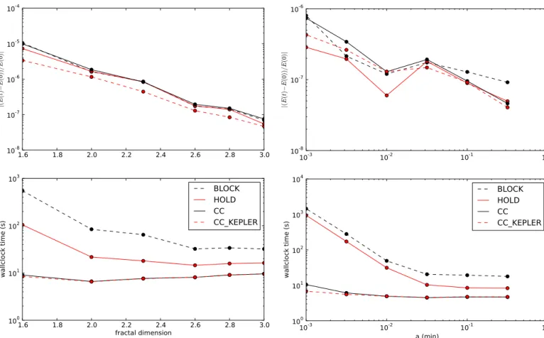
In Fig.6 we plot the energy error and runtime of the sim-ulation, averaged over 10 runs, as a function of the fractal di-mension f. While all integrators show similar energy conser-vation, CC and CC_KEPLER consistently outperform BLOCK and HOLD irrespective of fractal dimensions in terms of run-time. Further, runtime increases for decreasing fractal dimension for the BLOCK and HOLD integrators, while runtime remains essentially flat (and even decreases slightly) for decreasing frac-tal dimension for the CC and CC_KEPLER integrators.
3.4. Plummer sphere with binaries
We proceed by looking at how our methods perform on systems containing a large number of binaries. Specifically, we take a Plummer sphere and replace every particle with a binary system.
The positions and velocities of the particles are chosen such that under the absence of external perturbations, they would form a stable binary with a randomly oriented orbital plane, and a semi-major axis drawn uniformly in log space betweenlog(a) and−0.5. We integrate a system of 512 binaries (=1024 individ-ual particles) for 0.25N-body units withη=0.03.
Figure7visualises energy conservation and runtime of the initial conditions as a function of minimum semi-major axisa. For large a, the introduced binaries are generally unbounded, and the results are equivalent to evolving an ordinary Plummer sphere. As the minimum a decreases, the introduced binaries become bounded and their interactions start dominating in the integration time, leading to a significant advantage for CC and CC_KEPLER methods.
3.5. Cold collapse test
As a final test we evaluate the performance of our integrators in a cold collapse scenario. Specifically, we use the fractal initial conditions described in Sect.3.3with the initial velocities set to zero. We consider a “structured” case with the fractal dimension fd =1.6, and a “spherical” case with fd =3.0. We evolve initial
conditions for 2N-body time units. For the spherical case, this is past the moment of collapse that occurs around 1.5N-body time units. For the structured case the moment of collapse is less well-defined, as different substructures collapse at different times.
Fig. 5.A comparison of the HOLD, CC and CC_KEPLER methods on integrating an unsoftened 1024-body Plummer sphere through core collapse: conservation of the integrals of motion (top two rows), evolution of the mass distribution of the solution (third row) and wall-clock time (bottom left). Lagrangian radii are plotted for 90%, 50%, 10% and 1% of the system mass. Wall-clock times are normalised by CC_KEPLER at the first global time step (1/64-th of the simulation). On a laptop with a 1.3 GHz Intel Core i5 processor, CC_KEPLER integrates the first global time step in roughly 5 min while the entire simulation takes about 7 h.
GPU acceleration. We use a very small softening parameter (ε = 10−4) for Ph4 with GPU acceleration, and HiGPUS, as these run into severe slowdowns and/or crashes with unsoftened gravity – probably because of the limited precision of their GPU kernels. We set code-specific time step accuracy parameters to η=0.01 for CC/CC_KEPLER,η4 =0.1 for Ph4, andη4 =0.05 andη6=0.6 for HiGPUs.
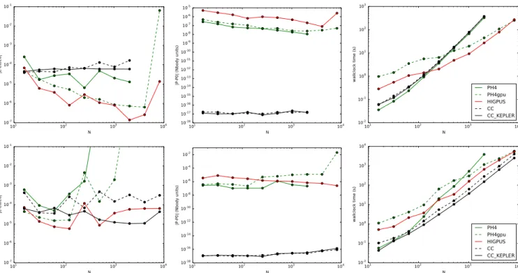
Figure 8 visualises energy conservation, momentum con-servation and the wall-clock time of the initial conditions as a function of the system size for structured and homogenous ini-tial conditions. In the spherical case, setups that take advantage of the GPU (PH4_gpu and HiGPUs) outperform the alterna-tives, but note that both CC and CC_KEPLER show very sim-ilar scaling to Ph4 without GPU acceleration. In contrast, for structured case, CC_KEPLER and CC show a marked speed up
in comparison with the conventional block time step schemes, being faster for this particular calculation than Ph4_GPU and HiGPUs, despite the latter having the advantage of using the GPU acceleration and integrating with softened gravity. The dif-ferences between the structured and the spherical cases highlight the relative advantage that the connected component approach has with respect to conventional block time steps when applied to multi-scale initial conditions.
4. Discussion
4.1. Using and extending the CC method
Fig. 6.Energy conservation (top) and runtime (bottom) for integrating a 1024-particle system of fractal initial conditions for 0.25N-body units as a function of the fractal dimension.
connected components of the time step graph (the CC split). We were motivated by the need for a more efficient divide-and-conquer strategy for reducing the intractable Hamiltonian (Eq. (18)) to the least possible number of analytically solvable Hamiltonians (Eqs. (7), (6)). In comparison to existing splitting methods, notably the HOLD split introduced inPelupessy et al. (2012), the CC split is particularly effective at splitting multi-scale systems. We have not encountered a situation where the HOLD split would be preferable over the CC split. The practical advantages of Hamiltonian splitting are similar to what is usually achieved with block time-steps. However, as our splitting meth-ods, including the CC method, do not extrapolate particle states for evaluating the total force acting on a particle, we conserve linear and angular momentum to machine precision.
We went on to show on the example of the CC_KEPLER method that the connected components partitioning has addi-tional uses beyond improved splitting efficiency. Specifically, we were able to incorporate regularisation of two-body close en-counters by simply checking for the condition where the suc-cessive partitioning leads to a connected component with two particles, and evolving the corresponding two-body Hamiltonian (Eq. (10)) using a dedicated Kepler solver. This approach can be extended to many-body close encounters by using a suitable specialised solver (or e.g. chain regularisation methods,Mikkola 2008) to evolve isolated Hamiltonians corresponding to con-nected components with certain properties. Possible selection criteria include having a specific number of particles and/or a maximum time step below a threshold value.
Fig. 7.Energy conservation (top) and runtime (bottom) for integrating 512-binary (=1024-particle) Plummer sphere for 0.25N-body units as a function of the initial semi-major axisa.
The numerical experiments of Sect.3were chosen to mainly study the splitting aspect of N-body integration. We focused on normalised performance metrics, and the scaling of the wall-clock time as a function of the “multi-scaleness” in the initial conditions. Our current implementations would benefit from additional optimisations typically used in production-level N-body codes. Specifically, there is inherent parallelism in the CC method, as recursive calls for evolving successively smaller closed Hamiltonians only affect the state of the particles in the “current” closed component. It may be possible to parallelise the method based on this property. However, tests show that a naive approach does not scale well due to load-balancing issues, as subsystems can vary substantially in size. Alternatively, it could be feasible to implement the CC method on a GPU, as the major components –N-body force evaluation (Portegies Zwart et al. 2007;Belleman et al. 2008;Capuzzo-Dolcetta et al. 2013) and graph processing algorithms (Harish & Narayanan 2007) – have individually been successfully implemented on GPUs.
Fig. 8.Energy conservation (left column), momentum (middle column) and wall-clock time (right column) as a function of system sizeNfor the cold collapse test. Thetop rowshows results for a homogenous sphere (fractal dimensionfd=3), while thebottom rowshows a highly structured
fractal (fd=1.6). We evolve the initial conditions for 2N-body time units, and plot the mean values across 5 runs. CC, CC_KEPLER and Ph4 use
unsoftened gravity (ε=0), while PH4_gpu and HIGPUS use very small softening (ε=10−4).
coordinates of the particles. As such, particles in the same con-nected component may occupy a “non-compact” region in phys-ical space, making multipole approximation difficult.
4.2. Formally optimal Hamiltonian splitting
The HOLD integrator determines the accuracy of a kick between particlesiand jfrom the particle-based time stepsτ(i) andτ(j). In the CC integrator the accuracy of a kick is determined by the time step graph generated directly from interaction-based time stepsτ(i,j). Could we further improve the splitting by applying kicks directly based on the interaction-specific time step crite-riaτ(i,j)?
We implemented this idea in an experimental integrator which we named the OK split (OK stands forOptimal Kick). The method partitions a list of allinteractionsin the system (based on a pivot time steph) just like the HOLD split partitions a list of allparticlesin the system. The partitioning is formally optimal in the sense that every kick is evaluated at the time step closest toτ(i,j) in the power of two hierarchy based on the pivot time steph. While the possibility of direct N-body integration with interaction-based time steps has been previously considered in Nitadori & Makino(2008), the OK split is the first workable im-plementation of this idea that we are aware of.
In numerical tests, the OK split is not competitive com-pared to other methods such as the CC split. For example, in the 1024-body smoothed Plummer sphere test from Sect.3.1, the relative energy error at the end of the simulation is around 10−2 (several orders of magnitude worse than HOLD and CC, but pos-sibly still enough for drawing statistically correct conclusions, Portegies Zwart & Boekholt 2014). The remaining integrals of motion are conserved at machine precision, as the OK split ap-plies kicks in pairs. Finally, the evolution of the mass distribution
is comparable to HOLD and CC with the OK split using fewer kick and time step evaluations.
Could we improve the OK split by changing the time step cri-teria? For example, considerτ(i,j)=min (τ(i), τ(j)) whereτis the particle-based time step criteria as defined inPelupessy et al. (2012). Formally, combining the OK split with τ(i,j) would result in a splitting with the exact same kicks and drifts as the HOLD integrator. This somewhat contrived example only serves the point of illustrating that the time step criteria can qualita-tively change the behaviour of the OK split. While it is unknown whether practical interaction-based time step criteria even exist, we do believe that a closer look at the various simplifications made during the derivation of the explicit and approximately time-symmetric time step criteria that we have used throughout this work (Eq. (19)) would serve as a good starting point.
Acknowledgements. We thank Guilherme Gonçalves Ferrari and the anonymous referee for a critical reading of the manuscript. This work was supported by the Netherlands Research Council NWO (Grants #643.200.503, #639.073.803 and #614.061.608) and by the Netherlands Research School for Astronomy (NOVA). Jürgen Jänes was supported by the Archimedes Foundation, Estonian Students’ Fund USA, Estonian Information Technology Foundation and Skype.
References
Ahmad, A., & Cohen, L. 1973, J. Comput. Phys., 12, 389 Barnes, J., & Hut, P. 1986, Nature, 324, 446
Bate, R. R., Mueller, D. D., & White, J. E. 1971, Fundamentals of Astrodynamics, Dover Books on Aeronautical Engineering Series (Dover Publications)
Belleman, R. G., Bédorf, J., & Portegies Zwart, S. F. 2008, New Astron., 13, 103 Capuzzo-Dolcetta, R., Spera, M., & Punzo, D. 2013, J. Comput. Phys., 236, 580 Cormen, T. H., Leiserson, C. E., Rivest, R. L., & Stein, C. 2001, Introduction to
Algorithms, 2nd edn. (MIT Press)
Gonçalves Ferrari, G., Boekholt, T., & Portegies Zwart, S. F. 2014, MNRAS, 440, 719
Goodwin, S. P., & Whitworth, A. P. 2004, A&A, 413, 929
Hairer, E., C., L., & Wanner, G. 2006, Geometric Numerical Integration: Structure-Preserving Algorithms for Ordinary Differential Equations (Springer Verlag)
Harish, P., & Narayanan, P. 2007, in High Performance Computing – HiPC 2007, eds. S. Aluru, M. Parashar, R. Badrinath, & V. Prasanna (Berlin, Heidelberg: Springer), Lect. Notes Comput. Sci., 4873, 197
Heggie, D. C., & Mathieu, R. D. 1986, in The Use of Supercomputers in Stellar Dynamics, eds. P. Hut, & S. L. W. McMillan (Berlin: Springer Verlag), Lect. Notes Phys., 267, 233
Konstantinidis, S., & Kokkotas, K. D. 2010, A&A, 522, A70 Makino, J. 1991, PASJ, 43, 859
McMillan, S. L. W. 1986, in The Use of Supercomputers in Stellar Dynamics, eds. P. Huts, & S. L. W. McMillan (Berlin: Springer Verlag), Lect. Notes Phys., 267, 156
Mikkola, S. 2008, in IAU Symp. 246, eds. E. Vesperini, M. Giersz, & A. Sills, 218
Nitadori, K., & Makino, J. 2008, New Astron., 13, 498 Oshino, S., Funato, Y., & Makino, J. 2011, PASJ, 63, 881
Pelupessy, F. I., Jänes, J., & Portegies Zwart, S. 2012, New Astron., 17, 711 Pelupessy, F. I., van Elteren, A., de Vries, N., et al. 2013, A&A, 557, A84 Portegies Zwart, S., & Boekholt, T. 2014, ApJ, 785, L3
Portegies Zwart, S., McMillan, S. L. W., van Elteren, E., Pelupessy, I., & de Vries, N. 2013, Comput. Phys. Commun., 183, 456
Portegies Zwart, S. F., Belleman, R. G., & Geldof, P. M. 2007, New Astron., 12, 641
Portegies Zwart, S. F., McMillan, S. L. W., & Gieles, M. 2010, ARA&A, 48, 431