EXPLORING THE MILKY WAY OUTER HALO GLOBULAR CLUSTERS AM 1 AND PYXIS∗
Brian L. Pohl
A dissertation submitted to the faculty of the University of North Carolina at Chapel Hill in partial fulfillment of the requirements for the degree of Doctor of Philosophy in the
Department of Physics and Astronomy.
Chapel Hill 2015
Approved by:
Bruce W. Carney
J. Christopher Clemens
Daniel Reichart
Fabian Heitsch
c 2015 Brian L. Pohl
ABSTRACT
BRIAN L. POHL: Exploring the Milky Way Outer Halo Globular Clusters AM 1 and Pyxis∗.
(Under the direction of Bruce W. Carney.)
In order to probe the origins and history of the Milky Way halo, I executed a photometric
survey of the outer halo globular clusters AM 1 and Pyxis using the southern astrophysical
research (SOAR) telescope. The principal goal of this investigation was to determine the
ages of these clusters, but the techniques employed in this process revealed other intrinsic
properties such as chemical composition. A total of 32.2 hours of data were obtained on
the program clusters, and observations of 22 stars from the Landolt (1992) catalogue were
used to transform the clusters to the Johnson-Cousins BV standard system. The resul-tant color-magnitude diagrams are used in conjunction with the reference globular cluster
M5 to determine the intrinsic properties of the program clusters. Three independent
age-determination techniques show agreement, consistent to within the error of the techniques,
that AM 1 is −1.0 Gyr younger than, and that Pyxis is coeval to, the reference cluster M5. The chemical properties of both clusters are found to be the same for both clusters,
[Fe/H] = −1.40and [α/Fe] = +0.4, similar to M5. The results are presented in terms of two outstanding issues regarding the outer halo; the second parameter problem and the issue of
accretion vs. in-situ formation.
∗Based on observations obtained at the Southern Astrophysical Research (SOAR) telescope, which is a joint
project of the Ministério da Ciência, Tecnologia, e Inovação (MCTI) da República Federativa do Brasil, the U.S. National Optical Astronomy Observatory (NOAO), the University of North Carolina at Chapel Hill (UNC), and Michigan State University (MSU).
To my loving wife Jalene who gave me the courage and support to pursue my dream,
ACKNOWLEDGMENTS
I am extremely grateful for the guidance, mentorship, and, above all, patience of my
advisor, Bruce Carney, and to the members of my committee, particularly Professors Reichart
and Clemens for technical advice regarding observing practices and data reduction.
I would also like to thank the individuals listed in this paragraph for assistance with
data acquisition. The lead observers Drs. Brad Barlow, Bruce Carney, Leslie Prochaska
Chamberlain, Haw Cheng, Bart Dunlap, Jesse Miner, and Jim Rose, and the SOAR onsite
observers Daniel Maturana, Alberto Pastén, Sergio Pizarro, Roberto Tighe, and Patricio
Ugarte. I am further grateful to Dr. Sean Points for technical assistance with SOAR data.
I am extremely grateful to Paula Borden and the science enrichment preparation program
(SEP), who provided financial support in the form of summer employment for the duration
of my doctoral program and for welcoming me into the SEP family.
I am thankful for advice, council, and friendship, through graduate school and beyond,
of Miles Blanton, Shane Brogan, Leslie Prochaska Chamberlain, Haw Cheng, Roseanne
Cheng, Matt Fleenor, Richard Longland, Jay Ihry, Sean Gidcumb, Michael Good, C. Bayard
Stringer, and Matt Wolboldt.
This project would not have succeeded without the love, support and encouragement of
my family. And finally, thank you for reading this.
TABLE OF CONTENTS
LIST OF FIGURES . . . ix
LIST OF TABLES . . . xiii
1 Introduction . . . 1
1.1 History of the Outer Halo . . . 2
1.1.1 The Second Parameter Problem . . . 4
1.2 The Globular Clusters . . . 9
1.2.1 The Extreme Outer Halo . . . 10
1.2.2 AM 1 . . . 16
1.2.3 Pyxis . . . 19
1.3 Purpose . . . 22
2 Data and Analysis . . . 25
2.1 Observations . . . 25
2.2 Data Reduction . . . 28
2.2.1 Calibration . . . 29
2.3 Photometry . . . 32
2.3.1 Aperture Photometry . . . 33
2.3.2 PSF Photometry . . . 34
2.3.3 Automation . . . 38
2.4 Catalog Assembly . . . 40
2.4.2 Fine Position Registration . . . 41
2.4.3 Median Images . . . 42
2.4.4 ALLFRAME . . . 43
2.4.5 Aperture Correction . . . 44
2.5 Reprocessing . . . 48
3 The Color Magnitude Diagrams . . . 49
3.1 Photometric Calibration . . . 49
3.1.1 Working Equations . . . 51
3.1.2 Determining coefficients . . . 55
3.1.3 Uncertainties . . . 58
3.2 Removal of Non-stellar Sources . . . 61
3.2.1 Sharp and χ¯ . . . 61
3.2.2 Statistical Subtraction . . . 64
3.3 Automation . . . 67
3.4 The Final CMDs . . . 67
4 Results . . . 69
4.1 Empirical . . . 69
4.2 Semi-Empirical Methods . . . 75
4.2.1 The Horizontal Method . . . 75
4.2.2 The Vertical Method . . . 85
4.3 Theoretical . . . 88
4.3.1 Input Parameters . . . 88
4.3.2 Input Parameter Constraints . . . 93
4.3.3 Results . . . 97
4.4 Summary . . . 99
5 Conclusions . . . 103
5.1 The Second Parameter Problem . . . 103
5.1.1 AM 1 . . . 103
5.1.2 Pyxis . . . 105
5.2 Accretion . . . 105
5.3 Future Work . . . 107
APPENDIX A Observing Logs . . . 109
APPENDIX B Source Code . . . 121
LIST OF FIGURES
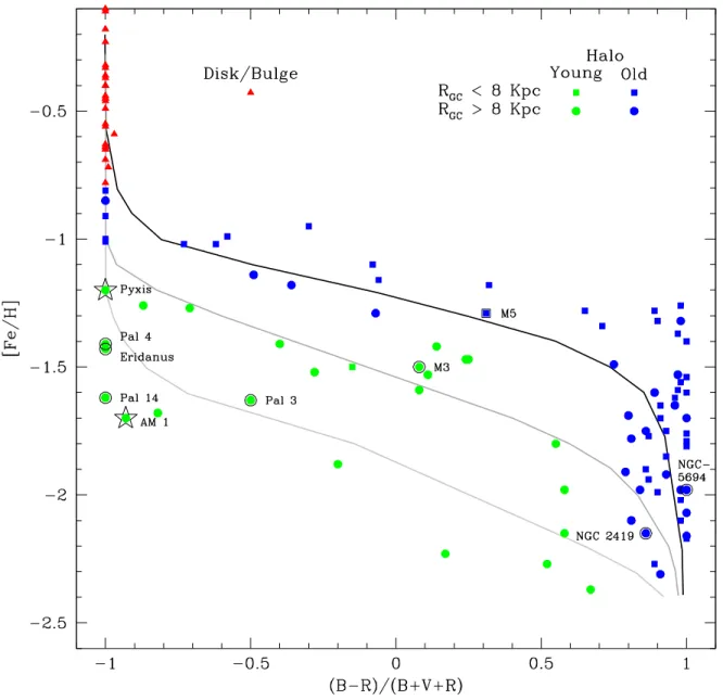
1.1 Example of a Lee Diagram constructed using the 2003 and 2010 revisions of Harris (1996). The solid black line represents the isochrone for the mean age of the inner halo population based on the models of Rey et al. (2001). The grey lines below represent relative age increments of −1.1 and −2.2 Gyr respec-tively. Metallicity alone distinguishes the disk/bulge population, whereas HB type offset between the mean inner halo age isochrone at a cluster’s metallicity distinguishes the young and old halo populations (see text for details). . . 8
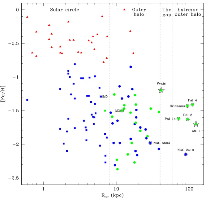
1.2 Metallicity versus galactocentric radius using data from Harris (1996, 2010 revision). The symbols match those defined in Figure 1.1. Note the presence of a metallicity gradient with 10 kpc that breaks at greater radii as well as the gap between ∼40and ∼60 kpc devoid of clusters. . . 11
2.1 The central20 2700region of AM 1. Upper left: An example of a bias subtracted, flat field corrected frame. This particular frame served as the master for theV
portion of ALLFRAME reductions. Upper right: The same frame after ALLSTAR
subtraction. Lower left: The median of 17 V frames. Lower right: Same as above but afterALLFRAME subtraction. . . 39
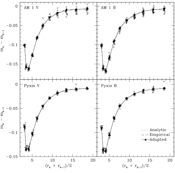
2.2 Curves of growth for both clusters in both filters. The open circles represent magnitude differences between adjacent apertures plotted versus the mean magnitude difference between the apertures in pixels. Artificial scatter is added to the horizontal scale to help distinguish the points. Fitting to the mean of the raw magnitude differences results in the empirical model and is more reliable for smaller apertures. Adjusting the parameters of an analytic function that best fits the stellar profile results in greater reliability at larger radii. The adopted model is the compromise between the two. . . 47
3.1 Filter throughput profiles for SOI circa October 2004 (solid lines) compared with those used by the Blanco 4m at CTIO to establish the standard system (dashed lines). Data for the SOI transmission curves are available from the SOAR website, and the CTIO data is from Tables 6 and 7 of Landolt (1992). The SOI filters have since been replaced, and updated transmission data are not yet available. . . 52
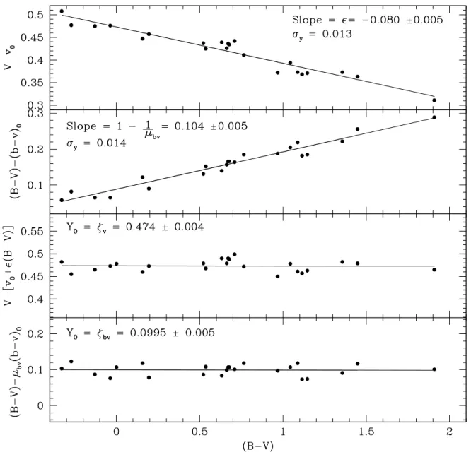
3.2 Linear fits used to determine the color transformation and offset terms. . . . 60
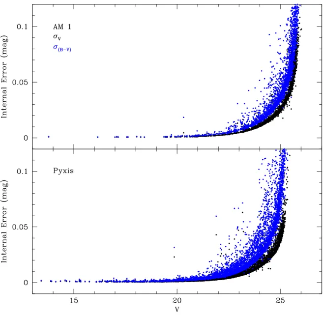
3.3 Internal errors of the averaged CMDs as a function of V magnitude. Black dots represent the uncertainty inV and blue dots in (B−V). . . 62
3.4 Comparison of cluster CMDs with and without the filtering criteria specified in equation 3.11. . . 63
3.5 Histograms used to determine the center of the clusters in pixel space. Stars were summed in 20 pixel columns and rows to determine thexandypixel cen-ters respectively. The difference in width of the best fitting gaussian between AM 1 and Pyxis is accounted for by the apparent size of each cluster. . . 65
3.6 Results of the statistical subtraction technique for AM 1. . . 66
3.7 The final color-magnitude diagrams for AM 1 and Pyxis. The error bars are only shown when the separation between brackets is visible. Only the
(B−V) errors typically meet this criteria, whereas in the V errors become distinguishable at the faintest magnitudes. . . 68
4.1 Fiducial sequences of M3 (Ferraro et al. 1997) and M5 (Sandquist et al. 1996) over plotting the data from which they were generated. The M3 data were obtained online and the M5 via private communication with the lead author. Known variable stars are excluded from the M3 data, and the M5 data are filtered by χaccording to Equation 3.11b. . . 72
4.2 Fiducial sequences of M3 and M5, the solid red and blue lines respectively, transformed to the same distance and reddening of the AM 1 and Pyxis. The insets expand the HB for each cluster indicated by the solid black rectangular regions in the main figures. The green line represents the average V magnitude of the stars in the HB region after a two sigma clipping algorithm. The open circles in the insets represent stars omitted by the sigma clipping filter. . . . 74
4.3 Gaussian fits to color histograms in the main sequence region of the clusters. The red error bars represent the average internal error of the stars in each magnitude bin scaled to the FWHM by Equation 4.2 and drawn at the half maximum level. Note the presence of a hump-like structure redward of the main peaks in Pyxis for V ≤22.9, most likely caused by binary stars. . . 79
4.5 (a) Best fitting isochrone to the ridge line points of Sandquist et al. (1996). The parameters also best match those used by VandenBerg et al. (2013). (b)
M5 best fitting isochrones varied by age registered to the common VBS points. The horizontal line at V −V+0.05 =−2.5 indicates the relative magnitude at
which the scale is determined. (c) Zoom in on the dotted line region of the lower left panel (b). (d)Best fitting line to the points in the panel above gives the color-age scale as -87.85 Gyr/mag. . . 84 4.6 The VBS method applied to AM 1 and Pyxis. The blue and red lines are the
fiducial sequences for M5 and M3 respectively. The orange cross represents the
V+0.05registration point and the green horizontal line represents theV+0.05−2.5
color-age scale level. Left panel inset: Zoom in on the RGB of AM 1. The solid blue line represents the best fit, second order polynomial to the M5 fiducial points (solid blue dots). The dashed blue line is the same polynomial shifted by−1.0Gyr according to the scale value derived in Figure 4.5. . . 86
4.7 The vertical method of VBLC applied to AM 1. Cyan lines represent the ages that best fit the SGB region within the red dotted region and blue lines best fit the MSTO. . . 89
4.8 Examples of how input parameters affect the DSED models. The blue lines match the best fitting parameters for AM 1 derived by D08b. For each panel, the non-varying parameters, listed in the lower right, correspond to the blue curves in the other panels. The exception is panel (d) which required an [α/Fe] of +0.4 as the other Y values are unavailable for [α/Fe] of +0.2 used in the other panels. The helium enrichment equation reflects the primordial helium mass fraction consistent with Spergel et al. (2003) plus the accumulation of helium along with the production of heavy metals at a rate of∆Y /∆Z = 1.54
(Dotter et al. 2008a, §3). . . 101
4.9 Best fitting isochrones for AM 1 and Pyxis. The green squares and error bars are the mode and FWHM of the ridge line points determined in §4.2.1 (see Figure 4.3.) The red plus signs represent stars studied in the radial velocity surveys of Suntzeff et al. (1985, S85) and Palma et al. (2000, P00) for AM 1 and Pyxis respectively. The red text corresponds to the star’s identifier code listed in Table 4.4. The color for P00-A matches that of the closest star in my catalog to the converted magnitude listed in Palma et al. (2000). . . 102
5.1 The same as Figure 1.1 but with the addition of extragalactic clusters from Mackey & Gilmore (2004, Table 2). The position of AM 1 and Pyxis based on the results of this work are shown as the solid, black pentagon and annotated as “Revised”. Their original positions based on the Harris (1996, 2003 and 2010 revisions) catalog are shown as open stars and annotated as “Harris”. . 104
5.2 The age-metallicity relationships (AMR) based on two different datasets. The results from this study are shown as green pentagons. The magenta circle represents M5. Clusters known or believed to be associated with the Canis Major (CMa) and Sagittarius (Sgr) dSph galaxies are indicated by the legend.
LIST OF TABLES
1.1 Extreme outer halo (EOH) globular clusters. . . 16
1.2 AM 1 candidate RR Lyrae stars reprinted from Ortolani (1984). . . 17
2.1 Target Coordinates . . . 25
2.2 Summary of observations . . . 27
2.3 An Example of PSF Stars for AM 1 . . . 37
2.4 Final Aperture Corrections . . . 46
3.1 CTIO Averaged Extinction Coefficients . . . 56
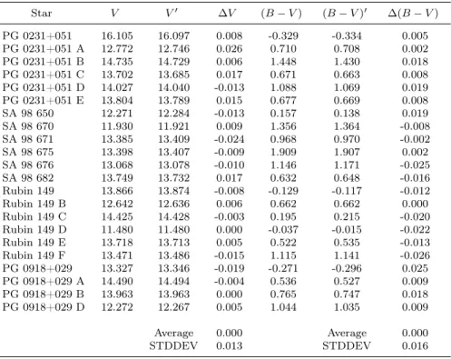
3.2 Standard star transformations from the night 2008-01-03 . . . 59
3.3 Color Transformation Coefficients . . . 59
4.1 Data from the Harris (1996) catalog . . . 73
4.2 Mean and modal ridgeline points . . . 78
4.3 Registration points for the VBS method. . . 81
4.4 Radial Velocities of the Brightest Red Giants . . . 96
4.5 Isochrone parameters compared to Dotter . . . 99
4.6 Summary of Results . . . 100
A.1 AM1 Observations log . . . 110
A.1 AM1 Observations log . . . 111
A.1 AM1 Observations log . . . 112
A.1 AM1 Observations log . . . 113
A.1 AM1 Observations log . . . 114
A.2 Pyxis Observations log . . . 115
A.2 Pyxis Observations log . . . 116
A.2 Pyxis Observations log . . . 117
A.2 Pyxis Observations log . . . 118
A.2 Pyxis Observations log . . . 119
Chapter 1 Introduction
On a clear, dark night, earthbound observers can see a narrow, dusty band spanning the
sky. This milky band we see from Earth represents the disk portion of our galaxy; indeed the
common perception of the Milky Way (MW) is only the spiral disk portion of the Galaxy,
but this notion betrays several other structures unknown to astronomers even a century ago.
The central region contains a bulge and a bar, and the disk itself is comprised of a thick
and thin component, the latter of which forms the classic “pinwheel” appearance associated
with spiral galaxies. Our sun lies within the thin disk about 8 kpc from the center of the
Galaxy, which is about three-quarters of the way to the edge of the canonical boundary of
the central portion of the MW (RGC ≤ 0.05×Rviral ∼ 12 kpc, Rix & Bovy 2013). Indeed
the popular conception of the MW structure would end there, but in fact the galaxy extends
another order of magnitude in galactocentric radius beyond our solar neighborhood into a
region called the halo.
The halo was first described by Harlow Shapely in a series of five classic papers published
in 1918 and 1919. He assumed the globular clusters contained therein were in arranged in
a spherical pattern around the center of the galaxy, and based on their apparent position
measured the Sun at 15 kpc from the center of the MW. Globular clusters (GC) are not the
only systems contained within the halo; dwarf spheroidal (dSph) galaxies, the Magellanic
Clouds, open clusters, individual stars and stellar “tidal streams”, or the disrupted debris of
evaporating GC and dSph systems, are found therein.
But what is the origin of the halo and what does its existence and structure tell us about
of the remnants of the protogalactic structure whose angular momentum and inclination
were sufficient to remain in circular orbit about the galactic center, or is it a repository for
remnants of accreted systems as more recent models of galactic evolution predict? Perhaps
a combination of both?
These questions remain unresolved in part due to the vast distances to, and hence
faint-ness of, the objects in the Halo. Many of the problems discussed below will be resolved as
more powerful telescopes and instruments come online. However, for the time being, the
halo represents a frontier of discovery about our galaxy.
Halos are observed around other galaxies as well, but the extraordinary distances to
ex-tragalactic systems inhibits the study of individual stars. Walter Baade was able to image
halo stars using photo plates during World War II, and HST has been able to resolve
indi-vidual stars as far away as M87. However, to thoroughly study a stellar system, to determine
its age, for example, using the techniques discussed in this work, the resolution of individual
stars at the main sequence turnoff (MSTO) and fainter are required. This is only practicable
for the nearest extragalactic systems such as the Magellanic clouds and local dwarf spheroidal
(dSph) galaxies. And while some of these dSph galaxies exist therein, the proximity of MW
halo is the best forest for which we may study the trees.
1.1 History of the Outer Halo
The story of the outer halo (OH) begins with Eggen, Lynden-Bell, & Sandage (1962,
ELS) who argued for the formation of the MW by dissipation collapse of a protogalactic
structure. They describe a scenario in which an enormous cloud of material collapses under
its common gravity. During the free fall portion of this collapse, the outermost stars and
clusters form and thus have highly eccentric orbits. As the cloud contracts, its angular
velocity increases and the shape flattens until a disk structure forms supported by its own
with increased ultraviolet excess with metallicity, which was assumed to be related to age,
leading to correlations with age and both orbital eccentricity and maximum height above
the galactic plane. Their conclusion that the youngest stars are confined to the plane of
the galaxy whereas the oldest stars are found almost everywhere support the dissipational
collapse model.
As the protogalaxy collapsed, the innermost stars, residing in a denser environment,
underwent rapid star formation and hence earlier enrichment of the interstellar medium.
Therefore a vertical as well as radial metallicity gradient serves as a testable observable for
the ELS model. Searle & Zinn (1978, SZ) undertook a survey of the abundances of 19 GCs,
most of which lie in the OH, and found no radial gradient beyondRGC >8 kpc (see Figure
1.2, which is an updated version of SZ Figure 6). Furthermore their classification of clusters
by morphological type, or how generally blue or red the horizontal branch (HB) stars are,
show a correlation with metallicity at inner galactic radii that breaks down forRGC >15kpc
(see their Figure 7). This shows that metallicity, the so called “first parameter”, dominates
HB morphology for IH clusters, but in the OH, some other mechanism is acting. The latter
effect is known as the “second parameter problem” and remains a topic of debate discussed
in § 1.1.1. The combination of these effects conflict with the ELS model, and SZ proposed a scenario for the formation of the OH by accretion of sub galactic “fragments.”
This debate persists over the past forty years fueled, as are many such great debates, by
the probability that both combatants contain portions of the truth. Follow-up studies by
Zinn (1980, 1993) and Lee, Demarque, & Zinn (1994, LDZ) provide evidence for the outer
halo forming by both processes.
The inner, older population of GCs formed from the dissipation collapse of the
proto-galaxy, and the outer, younger formed from some independent mechanism such as accretion
of extragalactic structures, the likeliest candidates being dSph galaxies and their associated
GC systems due to their continued proximity to the MW (see Marín-Franch et al. 2009, for
a recent review.)
Accretion as a component of galactic evolution comprises an important part of theΛCDM model of the universe (see Freeman & Bland-Hawthorn 2002, for a recent review.)
Obser-vational evidence of accreted satellite systems and their tidal debris streams continues to
accumulate. The most famous of these being the Sagittarius Dwarf Spheroidal (Sgr dSph)
and its associated tidal streams (see Belokurov et al. 2006 and references therein). Thus
little doubt remains that accretion occurred during the formation of the MW and remains
ongoing. How much of the halo is of extragalactic origin (Forbes & Bridges 2010), as well as
what exactly is being accreted (Geisler et al. 2007), remain open problems.
1.1.1 The Second Parameter Problem
As the name implies, horizontal branch stars share the same luminosity due to their
common core mass of ≈ 0.5M required to ignite helium burning. Generally speaking, the
color of a HB star depends on its envelope mass; the thicker the envelope, the larger its radius.
The energy of the core, related to its mass, must ultimately escape. Stellar luminosity (L) obeys the Stefan-Boltzmann relation for black bodies given by
L∝R2 T4. (1.1)
For fixed luminosity, as the radius (R) increases, temperature (T) must decrease. Thus more massive HB stellar envelopes have cooler surfaces and produce redder HB stars.
Due to the rapid evolutionary timescales of post main sequence stars, stars on the HB
began their ascent up the red giant branch (RGB) with roughly the same mass as stars
cur-rently at the MSTO. Pre-HB stellar core masses increase as helium piles up in the hydrogen
burning core, but stellar envelopes undergo mass loss of about 0.1 M, for example due to
solar winds, most prominently at the tip red giant evolutionary phase. RGB mass loss is
below regarding the parameters that influence HB morphology focus on the mass of MSTO
stars. The relevant physics behind these effects is discussed in §4.3.
Metallicity, the “first parameter”, dominates horizontal branch morphology due to its
influence on stars at the MSTO. Increased metallicity raises the mass of stars at the turnoff.
Thus more metal rich clusters classically show redder horizontal branches and vice-versa.
However, Sandage & Wildey (1967) and van den Bergh (1967) first noticed metal-poor GCs
with extremely red HBs. Some other mechanism, a “second parameter”, must be at work to
explain the anomalous HB morphologies.
The authors of the first studies of this phenomena put forth helium as the mechanism
for the second parameter. Increased helium also increases the luminosity of a main sequence
star by raising the mean molecular weight of the core. Greater luminosity means faster fuel
consumption and shorter stellar lifetimes, which lowers the mass of MSTO stars resulting in a
bluer HB. Age is another candidate due to its overwhelming influence on the mass of MSTO
stars. The main sequence is also a mass sequence as luminosity is directly proportional to
mass (a commonly cited but controversial relationship between the two is L ∝ M3.5). As the cluster ages, the turnoff luminosity, and mass, decreases. Other proposed mechanisms
include CNO abundance, stellar rotation rates and cluster central density (Ashman & Zeph
1998, §2.1.3). The ultimate color of a HB star depends on the extent of mass loss near the
tip of the RGB, a process that is poorly understood and difficult to measure. Thus all of
the above factors are speculative and based on observational correlation.
As studies of this mystery grew, various morphological indices developed as a statistical
measure of the relative number of stars blueward and redward of the instability strip (also
known as the RR Lyrae gap). An example of this quantitative measure of the HB morphology
is given as
HB Type = (B−R)
(B +V +R) (1.2)
where B, R and V represent the number of stars blueward, redward and within of the RR Lyrae gap respectively (Ashman & Zeph 1998, §2.1.3). Some authors, including SZ, use the
quantity B/(B+V).
Plots of metallicity vs. the morphological index, first constructed by SZ though commonly
called “Lee diagrams” due to their prominence in LDZ, show a correlation matching the first
parameter as the principle architect of HB type for GCs within the solar circle (RGC < 8
kpc) that break down at greater galactic radii.
An insight provided by Zinn (1993, see Figure 1) is that all the clusters in the inner halo,
which he defined as RGC <6 kpc, matched a nearly linear pattern in the Lee Diagram, but
the clusters beyond this galactocentric radius broke into two groups; one of which matched
the inner halo trend and another forming a parallel trend shifted by about 0.4 redward
in HB type. Assuming age as the second parameter, Zinn (1993) argued this latter group
represented a younger, and possibly accreted population.
An example of a Lee Diagram is shown in Figure 1.1 below. This is a reproduction of
Figure 5 of Mackey & Gilmore (2004), which is itself an updated version of Figure 7 of LDZ.
My figure uses HB type and metallicity data from the 2003 and 2010 revisions of the Harris
(1996) catalog1 respectively. The figure does not include every entry in the catalog, merely
the set of clusters for which both HB type and metallicity data are available.
The original trend used by Zinn (1993) to fit the inner halo was drawn by hand, but
isochrones based on HB model evolution codes evolved over the years culminating with
those developed by Rey, Yoon, Lee, Chaboyer, & Sarajedini (2001). These isochrones2 are
shown as solid lines in Figure 1.1, the darkest of which matches the mean age of the inner
halo (now canonically defined as RGC ≤ 8 kpc) and the lower grey lines represent relative
1HB type data are unlisted in the 2010 revision, presumably because the reliability of measurements from
2003 obviate revision.
2Private communication with Soo-Chang Rey revealed that the authors misplaced the original data used to
age increments of −1.1 and −2.2Gyr respectively.
A modification of the criteria originally specified by Zinn (1993) distinguishes the
pop-ulations in Figure 1.1. The exact algorithm, adapted from Keller et al. (2012), is given
as
for each c l u s t e r if ([ Fe / H ] > -0.8)
C l a s s i f y as Disk / B u l g e p o p l u a t i o n
else if ( HB type - HB F i d u c i a l < -0.3) C l a s s i f y as Y o u n g Halo p o p u l a t i o n
else
C l a s s i f y as Old Halo
where HB Fiducial is the isochrone matching the mean inner halo age (the black line in
Figure 1.1).
SZ’s observation of the second parameter association with position in the galaxy led them
to conclude that age primarily drives HB morphology in the OH, as HB of older clusters
evolved from stars with less overall mass. The age-as-second-parameter argument couples
nicely with the accretion model of galaxy evolution because the observed age difference
between the OH and IH of≈2Gyr is an order of magnitude greater than the timescale for a free-fall collapse predicted by ELS. However, the observed age difference is too short a time
interval compared with dynamical simulations (see the introduction of Dotter et al. 2010a,
for a recent and comprehensive review).
Furthermore, MSTO measured ages appear to differ among clusters of similar metallicity.
Clusters that share similar metallicities but widely different HB types are referred to as
“second parameter pairs”, the classic example of which being NGC 288 and NGC 362. Both
clusters share a similar metallicity of −1.32 and −1.30 respectively (Carretta et al. 2009), but NGC 288 has an exclusively blue HB and NGC 362 is mostly red. Catelan, Bellazzini,
Landsman, Ferraro, Pecci, & Galleti (2001) showed an age difference of 2±1Gyr that could explain the variation in HB morphology. However, most recently, VandenBerg, Brogaard,
Leaman, & Casagrande (2013), employing the most recent and accurate technique for relative
age determination discussed in further in §4.2.2, find an age difference between the clusters of
only0.75±0.45Gyr. They argue that, in addition to age, enrichment variations in helium or Mg and Si may be at work. Additionally, analyses of the MSTO derived ages for several such
second parameter pairs show enough variation that HB morphology cannot be explained by
age alone (see §7 of Catelan 2009).
Thus some other factor or set of factors in addition to or perhaps exclusive of age may
be required. Most recently, Dotter (2013) points out one of the reasons the problem remains
so intractable is that the approach one takes biases the conclusion. Indeed the study of
the second parameter problem remains an open debate. That the second parameter effect
appears characteristic of the OH is of greater concern to this work than the exact mechanisms
behind it.
1.2 The Globular Clusters
Globular clusters are classically believed to be simple systems of stars that formed from
the same material at the same time. As such, they are coeval and homogenous in
composi-tion, which makes them among the few systems for which reliable ages may be determined.
Furthermore, globular clusters are compact enough to survive the accretion process despite
complete evaporation by their parent system. This makes them analogous to fossil relics of
our galaxy’s past.
Why study AM 1 and Pyxis? As discussed in §1.2.2 and §1.2.3, at the onset of data
acquisition for this project in the fall of 2008, little was known about either cluster. AM
1, being the most distant and hence faintest GC, serves as an excellent capability indicator
for the, as then newly commissioned, Southern Astrophysical Research Telescope (SOAR).
As shown in Table 2.1, both clusters are of sufficient southern declination for SOAR to
practically survey.
In the course of investigating the background of these clusters, some interesting scientific
motivations arise. Both clusters show the second parameter effect and have apparently young
ages, but their position in the Galaxy is curious in itself. Figure 1.2, an updated version
of the same plot by SZ showing galactocentric distance vs. metallicity, shows a curious
region between 40/ RGC /60 kpc, labeled as “the gap,” that contains no currently known
clusters. The logarithmic scale of the horizontal axis betrays the relative size of “the gap;”
it is 2.5 times wider than the radius of the solar circle. Figure 1.2 uses the same data and
symbol convention as Figure 1.1. As the most distant cluster identified with the MW, AM 1
contains the outer region beyond the gap along with only five other clusters (see Table 1.1.)
This outer region also occupies the nearest dSph galaxies making the clusters therein likely
accretion remnants. At 42 kpc, Pyxis lies at the innermost edge of the gap and cannot be so
easily identified as an accretion candidate by position alone. Thus similarities between the
current properties of Pyxis and AM 1 point to a common mechanism of origin.
Before embarking on our own exploration of these clusters, let us begin with the state
of knowledge to date regarding all outermost halo clusters. The remainder of this section
summarizes work performed by other authors with an emphasis on measurements relevant
to age and chemical composition.
1.2.1 The Extreme Outer Halo
The outermost part of the halo, beyond the “the gap,” is frequently referred to as the
“extreme outer halo” (EOH). To provide some context for the study of AM 1 and Pyxis,
this section probes the most recent studies of the clusters in this region. We keep an eye
trained on the issues of what constitutes the typical characteristics of an EOH cluster and
which clusters are unique. The key issues to note include whether or not the cluster shows
Figure 1.2 Metallicity versus galactocentric radius using data from Harris (1996, 2010 revi-sion). The symbols match those defined in Figure 1.1. Note the presence of a metallicity gradient with 10 kpc that breaks at greater radii as well as the gap between ∼40and ∼60
kpc devoid of clusters.
other clusters in the outer halo.
From a chemical perspective, a look at Figure 1.2 shows that the most metal rich clusters
lie within the solar circle and, though there is quite a bit of spread, the OH appears to be
restricted to the range −2.0 / [Fe/H] / −1.0. Carney (1996) notes that the OH clusters share a common [α/Fe] = +0.3. §4.3.1 discusses the specific effects of age, metallicity, helium, and αenhancements of the cluster in the observational plane as well as the relevant physics. In the discussion that follows, we begin with the EOH clusters that appear “typical” in a
chemical sense and conclude with the outliers.
It is also worth noting the chemical inventory of nearby dSph galaxies as a number of
clusters in the EOH are considered accretion relics. Venn et al. (2004) notes that dSph
galaxies share very low α (very nearly solar) enhancements and are simultaneously more metal rich than the MW. She uses these results to argue against the idea of an accreted
EOH population.
Palomar 3
We begin our survey of the EOH with what appears to be the most generic sample.
Palomar 3 resides at a distance of RGC ' 92kpc and is about 1.5 to 2.0 Gyr younger than
M3 according to Stetson et al. (1999). Koch et al. (2009) reports [Fe/H] = −1.58±0.13
and [α/Fe] = 0.35±0.23. They report all chemical abundances fully consistent with the clusters and field stars of the outer halo. Indeed, the title of their paper, “All Quiet in
the Outer Halo”, implies that this cluster as a benchmark standard of ordinariness for this
neighborhood.
Palomar 4
A galactocentric distance of 109 kpc (Stetson et al. 1999) and a half light radius a full
order of magnitude greater than that of a typical GC distinguishes Palomar 4 as among the
most distant and diffuse globular clusters known. Stetson et al. (1999) determined its age
Coupled with its relatively low total luminosity, these properties make it similar in many
ways to UFD. Koch & Côté (2010) obtained high resolution spectra of 19 RGB stars using
the Keck/HIRES spectrograph. They report[Fe/H] =−1.41±0.17and[α/FE] = 0.38±0.11, the latter being consistent with the rest of the EOH clusters with the exception of NGC 2419.
Its extremely red HB places it comfortably in the territory of the Lee Diagram occupied by
its neighbors. Though they report an unusual [Mg/Ca] abundance, Koch & Côté (2010) find
its overall chemical pattern in agreement with the other EOH clusters; they even go as far
as to describe Palomar 3 and Palomar 4 as “twins” due to their nearly identical chemistry,
distance and half light radii.
Palomar 14
At a heliocentric distance of∼71±2kpc (Sollima et al. 2011), Palomar 14 is the innermost EOH cluster. Like the other clusters its neighborhood, it is faint, diffuse, displays a red HB
and is about 2 Gyr younger than M3 (Dotter et al. 2008b). High resolution spectroscopy by
Caliskan et al. (2012) reports [Fe/H]=−1.44±0.03and[α/Fe] = 0.34±0.17. These results as well as the other elemental ratios show Palomar 14 as nearly identical in chemical abundances
as the EOH clusters Palomar 3 and Palomar 4. One of the most striking discoveries regarding
this cluster is the presence of two tidal tails (Sollima et al. 2011). The chemical similarity
of this cluster to the other Palomar clusters in the EOH, as well as the presence of its tidal
tails, lead the authors of both studies to conclude Palomar 14 is a likely an accretion relic
from an evaporated dSph parent galaxy.
Eridanus
The most comprehensive, though aging, review of Eridanus is given by Stetson et al.
(1999). Its metallicity (−1.42±0.08 dex, Carretta et al. 2009, and references therein), dis-tance and age (Catelan 1999) are quite similar to Palomar 4, enough so that investigations in
to the second parameter problem they are cited as classical second parameter pairs (Catelan
2009). Much like its second parameter cousin, everything about this cluster seems typical of
the EOH. However, no high resolution spectroscopic studies yet exist for this cluster. The
metallicity cited above ultimately comes from Calcium II triplet line strength analysis by
Armandroff & Da Costa (1991).
Here ends the discussion of the “typical” EOH clusters. What follows represent the
clusters that are dissimilar to the others.
NGC 5694
Though its current galactocentric distance of 30 kpc, similar to that of Pyxis, excludes it
from the canonical EOH group, its velocity with respect to the galactic center of −273±13
km/s lead Harris & Hesser (1976) to believe it an interloper from the EOH whose orbit
extends to ∼ 100 kpc. Lee, Lopez-Morales, & Carney (2006), making use of the chemi-cal tagging technique with high resolution spectra of a single red giant in the cluster,
no-ticed anomalously low values of [α/Fe] and [Cu/Fe] compared to globular clusters of similar metallicity and concluded the cluster is likely of extragalactic origin. Mucciarelli et al.
(2013) extended the study to include a total of six red giants in the cluster and measured
[Fe/H] = −1.98±0.03 and [α/Fe] = 0.02±0.02. Its low metallicity and blue dominated HB place it in the lower right of the Lee Diagram, quite apart from the EOH clusters that
occupy the lower left. Additionally its solar α enhancement distinguishes it chemically from the rest of the outer halo. Mucciarelli et al. (2013) ultimately agrees with the conclusions of
Lee et al. (2006) that NGC 5694 is an interloper from the EOH and of extragalactic origin,
but it formed in an environment unique to the rest of the EOH which are believed to be relics
of dSphs. Ultra Faint Dwarf (UFD) galaxies share a similar combination of poor metallicity
potential chemical sibling.
NGC 2419
We conclude this tour of the EOH with the most interesting cluster of them all. Second
in luminosity among globular clusters beyond RGC > 15 kpc to M54, which is known to
be the core of the Sgr dSph, NGC 2419 is more massive, by an order of magnitude, than
all the EOH globular clusters combined (Borissova et al. 1996, see Table 7). With a blue
dominated HB, it occupies the opposite side of the Lee Diagram than the rest of the EOH
clusters with the exception of the interloper NGC 5694 which is suspected of being a UFD.
Chemical analysis by Cohen et al. (2011) show a mean [Fe/H]=−2.06±0.10 and [α/Fe] = 0.19±0.4; both low compared to the rest of the EOH. A closer look at the chemical inventory by Cohen & Kirby (2012) showed an anomalous depletion of magnesium in a third of stars in
the cluster. The authors describe this anomaly as “unprecedented” among globular clusters,
leading them to conclude that NGC 2419, like its luminous cousin M54, is the nucleated core
of a dSph.
Very recently, Mucciarelli et al. (2015) also discovered a K–Mg anti-correlation in NGC
2808, a cluster known to have three distinct populations (Piotto et al. 2007). The three
populations in NGC 2808 are believed to be subsequent generations of stars formed from the
gravitationally bound debris of primordial stars. As such, Mucciarelli et al. (2015) attribute
the K–Mg anti-correlation to a self-enrichment scenario. While this does not exclude the
possibility of NGC 2419 being a nucleated dSph, indeed a dSph would have no trouble
providing enough gravitational potential to retain the gas from early generations of stars,
the K–Mg anti-correlation, in and of itself, no longer provides evidence for this classification.
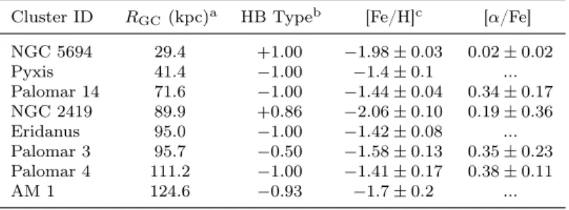
Table 1.1. Extreme outer halo (EOH) globular clusters.
Cluster ID RGC(kpc)a HB Typeb [Fe/H]c [α/Fe]
NGC 5694 29.4 +1.00 −1.98±0.03 0.02±0.02
Pyxis 41.4 −1.00 −1.4±0.1 ...
Palomar 14 71.6 −1.00 −1.44±0.04 0.34±0.17 NGC 2419 89.9 +0.86 −2.06±0.10 0.19±0.36 Eridanus 95.0 −1.00 −1.42±0.08 ... Palomar 3 95.7 −0.50 −1.58±0.13 0.35±0.23 Palomar 4 111.2 −1.00 −1.41±0.17 0.38±0.11
AM 1 124.6 −0.93 −1.7±0.2 ...
aDistances from Harris (1996, 2010 revision)
bHorizontal branch types of the form(B−R)/(B+V+R)from Harris
(1996, 2003 revision)
cWhenever possible, metallicities and α enhancements are from the
latest high resolution spectroscopic studies. References contained in the text.
Summary
With the exceptions of NGC 2419 and NGC 5694, the extreme outer halo clusters show
nearly uniform metallicity (−1.6.[Fe/H].−1.4) and mean alpha element (0.3.[α/Fe]. 0.4) enhancements as shown in Table 1.1. The authors of the most recent studies of nearly all these clusters argue for their extragalactic origin.
1.2.2 AM 1
Though previously identified as ESO-201-SC by Holmberg & Lauberts (1975) during
their survey of the ESO “Quick Blue” plates, the designation Arp-Madore-1, or simply AM-1,
assigned by Madore & Arp (1979) persists because they produced a color-magnitude diagram
(CMD). They discovered three faint stellar clusters among the IIIa-J plates acquired by the
Australian UK Schmidt Telescope Unit. Based on the limiting magnitude of mJ = 20.5 on the ESO discovery plates and an assumed color of(B−V) = 1.4for red giants, they estimated that the brightest stars have a magnitude ofB = 21.2. Coupled with an absolute magnitude
Table 1.2. AM 1 candidate RR Lyrae stars reprinted from Ortolani (1984).
Star ID∗ V (B-V)
12 21.02 0.33
19 21.27 0.28
50 21.10 0.40
67 21.16 0.46
83 21.07 0.45
Note. — ∗ The Star ID column is Ortolani’s designa-tion. His paper provides a finder chart
on the cosecant law3 of Harris & Racine (1979), they reported a tentative distance of 300
kpc.
Ortolani (1984) obtained BV photometry using the 1.5 meter ESO telescope at La Silla to a limiting magnitude of V = 23, sufficient to identify the horizontal branch (HB). They also identified 5 possible RR Lyrae (RRL) stars based on their de-reddened color lying
within the RRL gap [1.8≤(B−V)≤4.2]. However, they assume an interstellar extinction term of E(B − V) = 0.03 based on the cosecant law. All subsequent authors assumed interstellar extinction to be negligible for this object [E(B −V) = 0.00]. Without the extinction correction, two of their RRL candidates fall outside the RRL gap. Table 1.2 lists
non-extinction corrected colors for the candidate RRLs.
Based on an assumed < MV >= 0.6 for the RR Lyraes, Orlotani reported a distance of RGC = 123±10kpc. Using the color index of the RGB at the HB of(B−V)0,g = 0.76±0.08
he estimates a metallicity of [Me/H] = −1.6± 0.4 based on the average value of three techniques.
Working independently using the CTIO 4m telescope, Aaronson, Schommer, & Olszewski
(1984) obtained a total exposure of 3000 seconds each in B andV (though only 2000 of each
3E(B−V) =K
bv[1−exp(−Z/Z0)]×csc|b|whereZ0is the scale height of the Galactic extinction layer and Kbv is a derived constant equal to 0.056 and 0.040 for the north and south poles (Racine & Harris 1989, Equation 2).
were on nights designated as “clear”). They show a well-defined HB but do not identify any
candidate RRL stars as the blue edge of their HB lies outside the RRL gap [(B−V) = 0.47]. They assume no interstellar reddening [E(B −V) = 0.00] based on the maps of Burstein & Heiles (1982).
Assuming MV(HB) = 0.6, they computed a distance ofRGC= 118±2kpc. Their upper
RGB is heavily contaminated by field stars, leaving them confident of only one upper RGB
star in their sample of cluster members. Based on a fit of the upper RBG heavily weighted
by this one star, they estimated a metallicity of [Fe/H] = −1.8±0.3.
Both Aaronson et al. (1984) and Ortolani (1984) measurements of distance and metallicity
agree within the errors, something Orlotani points out as support for their results. Though
the discrepancy in the reddening between the two authors raises an eyebrow. Due to the
extremely red nature of the HB, both authors identify AM 1 as a good second parameter
cluster in need of future studies, particularly with regard to spectroscopy.
The only spectroscopic study of AM 1 was undertaken by Suntzeff, Olszewski, & Stetson
(1985). Using the 2.5 m du Pont telescope at Las Campanatas Observatory in November of
1983, they obtained spectra on the two brightest stars in the cluster (shown as red plus
sym-bols in Figure 4.9). Based on the line strengths of the Calcium II H and K line strengths, they
determined a metallicity of [Fe/H] =−1.7±0.2. They further determined a Galactocentric radial velocity of −41km/s.
Hilker (2006) obtained VLT data in BV toV ≤22.9. His CMD shows a well defined HB and RGB suitable for fitting with the Yonsei-Yale (Y2, Kim et al. 2002) isochrones. However,
Aaronson’s metallicity estimate of−1.8did not adequately fit the data. Instead a metallicity of −1.4 was used for the best fitting isochrones. Other fitting parameters fix the age at 11 Gyr, and [α/Fe] = 0.3 dex. He further used an an artificial color shift of−0.01to correct an offset between his best fitted isochrone and the data that he ascribes to reddening.
to establish reliable cluster members and good positions for further spectroscopic work on
individual stars, necessary to lay to rest many questions regarding the chemical history of
the cluster and its origin. His final catalog has positions reported to 0.01" RA and 0.1" Dec.
Finally and most recently, Dotter et al. (2008b) obtained HST data in V andI (or in the HST parlance, F555W and F814W respectively) down to 28th magnitude in V. In addition to the RGB and HB, the MSTO is clearly visible as well as some blue stragglers that appear
interesting as well.
Because Hilker’s CMD’s does not include the MSTO, they are skeptical of his metallicity
estimate and use a baseline of [Fe/H] = −1.5as their baseline for a differential technique of isochrone fitting using M3 as a comparison. They caution that this technique is only valid in
the extent that M3 and AM 1 are of the same composition, a point they repeatedly stress as
need for follow up high resolution spectroscopy. Their final values are [Fe/H] =−1.5, [α/Fe] = +0.2, age = 11.1 Gyr or 1.5 Gyr younger than the comparison cluster M3.
Their paper shows that all six GCs with RGC >50kpc are younger than the inner halo
clusters, evidence, they argue, that all such clusters were accreted and the best candidate for
the second-parameter is age. But they stress the need for direct metallicity measurements are
necessary. Indeed four different authors using different techniques arrived at four different
values.
1.2.3 Pyxis
While searching the Palomar Observatory Sky Survey for planetary nebulae, Weinberger
(1995) discovered several new objects worthy of followup study including a possible satellite
globular cluster or dwarf spheroidal galaxy. Follow-up work by Da Costa (1995) and Irwin,
Demers, & Kunkel (1995) confirmed the object as an outer halo GC; the former investigator
designated it as “C J0907-372 (Pyxis)” and the latter suggested the simply Pyxis.
Da Costa (1995) obtained 900 second B and 300 second R CCD images using the ≈ 3.9 meter Anglo Australian Telescope (AAT). Poor seeing (2.001) restricted their limiting magnitude of their CMD, their Figure 3, to R ≈22mag. However, their large overall FOV compared to the SOAR optical imager (SOI) allowed them to construct a field star CMD,
shown as the lower panel of Figure 3. The fact that their FOV encompassed the entire cluster
allowed them to fit a King (1966) model to the surface density profile and determine the core
radius of 8300. Their inability to fully capture the MSTO restricted their conclusions about age to a lower limit on magnitude difference between the HB and MSTO of∆RHB−TO ≥3.25,
leaving them no reason to suspect the cluster’s age is radically different compared to the rest
of the halo GCs which have values of ∼ 3.5 (Green & Norris 1990). Fitting RGB fiducial sequences of NGC 362 and NGC 6397 established a galactocentric distance ofRGC ≈37kpc,
but the disparity of metallicities between the fiducial clusters, [Fe/H] = −1.28 and −1.91
respectively, while both providing good matches to the Pyxis RGB, restrict their conclusions
metallicity to the range bound by those of the reference clusters and extinction to the interval
of 0.25≤E(B−V)≤0.40.
Working independently, Irwin et al. (1995) acquired B, R and I CCD data using the 2.5 meter du Pont telescope at Las Campas Observatory. Their Figure 3 shows a CMD
with a limiting magnitude of R ≈ 23 mag, or about a half magnitude below the MSTO. Application of the Yale isochrones (Green, Demarque, & King 1987) resulted in a metallicity
of [Fe/H] = −1.1± 0.3 and an age of 13±3 Gyr assuming a reddening of E(B −V) = 0.19±0.04 consistent (though barely) with the value of ≈ 0.23 derived from the maps of Burstein & Heiles (1982). The metallicity agrees with the value of −1.0±0.3 determined by the dereddened color of the RGB at the magnitude of the HB ((B −V)0,g = 0.9±0.1).
Their absolute age measurement is subject to the uncertainties of the Yale (or indeed any)
and theMV(RR) = 0.15[Fe/H] + 0.72 relationship of Walker (1992).
Acknowledging the previous investigators’ efforts as good initial reconnaissances of Pyxis,
Sarajedini & Geisler (1996) set out to construct a CMD faint enough to fully establish the
MSTO and determine the age of the cluster. They obtained single 30 and 600 second
exposures in R and 60 and 1200 second exposures in B using the CTIO Blanco 4 meter telescope on a night with good seeing (0.009 and 1.001 respectively). Their CMD (Figure 2) extends toR ≈24or about a magnitude below the MSTO. The 14.07 FOV allowed them to fully sample the field star CMD (Figure 3) and restrict their sample to stars within twice
the core radius established by Da Costa (1995). Making use of the simultaneous reddening
and metallicity method (SRM, Sarajedini 1994) adapted for the B, R system, they derived
[Fe/H] = −1.20±0.15 and E(B −V) = 0.21±0.03, both of which are in good agreement with Irwin et al. (1995) and Da Costa (1995). Employing a technique involving the color
difference between the HB and the RGB (Sarajedini et al. 1995), they reported an age of
13.3 ±1.3 Gyr subject to the usual systematic errors associated with GC absolute ages. More convincing are the relative ages derived by overlaying fiducial sequences, shown in
their Figure 5, that show Pyxis to be of similar age to NGC 362 and significantly younger
than NGC 288. Recall that NGC 288/362 are the classic second parameter pair as they share
similar metallicity but drastically different HB types (Catelan et al. 2001). Finally, using
the mean R magnitude of 27 HB stars and the absolute magnitude relation of Lee (1990),
MV(RR) = 0.17[Fe/H] + 0.79, they reported a Galactocentric distance of 41 kpc.
All the investigations above mentioned the need for spectroscopic measurements, to which
Palma, Kunkel, & Majewski (2000) answered the call, obtaining spectra with a 1200 line/mm
grating spectrograph configured for a 7700–8750 Å wavelength range and roughly1.3Å/pixel detector resolution at the 2.5 meter du Pont Telescope at Las Campanas. Motivated to
determine the orbital kinematics in order to test the hypothesis of Pyxis as a captured
LMC object put forward by Irwin et al. (1995) and later supported by Palma, Majewski,
& Johnston (2002, submitted at the time), radial velocities comprised their primary goal.
Their exposure times provided sufficient SNR for radial velocities of the brightest six stars,
labeled A through F in order of brightness, from which they obtain a mean radial velocity
of 39.5 km/s after excluding one outlier, Pyxis D, from their sample. Only the brightest star, Pyxis A, provided sufficient SNR for metallicity estimation. Following the technique
outlined by Rutledge et al. (1997), Calcium II equivalent width measurements, W0, yielded a metallicity of[Fe/H] =−1.4±0.1 dex.
Finally, Dotter et al. (2011) obtained HST data in the F606W and F814W (or V and
I) filters for Pyxis along with five other GCs in the interval 15 ≤ RGC ≤ 50 kpc. Their
CMD (Figure 3) extends to 26th magnitude inV (F606W), or∼4.5mag below the MSTO. Applying the age determination technique described by Dotter et al. (2010b, section 4.2)
using the Dartmouth Stellar Evolution Database (Dotter et al. 2008a, DSED) isochrones,
they reported an age of 11.5±0.1 Gyr, V magnitude distance modulus (DMV) of 18.64, E(B−V) = 0.25, [Fe/H] =−1.5, and [α/Fe] = 0.2(see their Table 3).
1.3 Purpose
To best understand the origins of AM 1 and Pyxis and their insights into the formation of
the outer halo, we must first ascertain their physical properties as best as possible. Detailed
chemical abundance and kinematics measurements could lay to rest many of these questions
through “chemical tagging” (see, for example, Geisler, Wallerstein, Smith, & Casetti-Dinescu
2007; Brewer & Carney 2006), if only the instrumentation existed to obtain the requisite high
resolution and SNR spectra.
Thus we employ the best tools at our disposal for the study of this frontier. The SOAR
telescope provides sufficient aperture to study such faint objects, and our access to roughly
one or two nights per month each target is available allows for an unprecedented amount
exhaust the possibilities of ground-based instrumentation for AM 1 and Pyxis, making future
applications for time on space based instrumentation more compelling, if deemed necessary.
Wide bandpass photometry makes the most efficient use of telescope aperture and time
by exploiting the greatest amount of light. The consequence is that chemical abundance
measurements must be made in an indirect fashion. Photometrically derived parameters
such as metallicity are worthwhile goals in that they serve as starting points, and verification
tests, for more direct techniques. Therefore we set out on this campaign with the goal of
deriving such properties with the caveat that their conclusive determination will not be
available until instruments capable of high resolution spectroscopy (or perhaps some as yet
unforeseen technique) are available.
The age of a globular cluster is the most worthwhile and reliable measurement photometry
reveals. Being classically considered coeval systems4, the stars therein show all stages of
stellar evolution. A globular cluster color-magnitude diagram (CMD) shows a main sequence,
subgiant and red-giant branches, horizontal branches and asymptotic giant branches. As
discussed later, comparisons of stars at different evolutionary phases in the CMD reveals the
age of the cluster as a whole. Revisiting the analogy of globular clusters as fossils, revelations
about the age of a cluster provide clues about its origins and history inasmuch as carbon
dating reveals the same of a biological fossil.
The purpose of this endeavor, therefore, is reliable age determination for AM 1 and Pyxis
using a variety of techniques. In the process, we hope to discover or confirm other intrinsic
properties of the clusters such as metallicity andαelement enhancement as well as extrinsic properties of distance and interstellar extinction.
Chapter Two discusses the observing program and the data reduction process. Chapter
Three describes the calibration of the stars to the standard system and the construction of
the CMDs. In Chapter Four, I bring to bear three independent techniques for determining
4There are a growing number of clusters that show multiple populations betraying the notion that all GCs
are coeval systems. See Piotto (2009) for a review.
Chapter 2 Data and Analysis
2.1 Observations
Several individuals, including myself, obtained the data between the fall of 2007 and
spring of 2009 using the Southern Astrophysical Research (SOAR) telescope, a 4.1 meter
aperture telescope located on Cerro Panchón, Chile, at an altitude of 2,700 m and south latitude of −30.2◦. In order minimize the effects of the atmosphere on the star light, we
maintained an observing constraint of an airmass, X, less than 2, or a maximum of 30◦ from the zenith. SOAR’s south latitude restricts the preferred (X < 2) observing declination range to 0◦ ≥ δ ≥ −60◦
, ideal for southern hemisphere targets due to the availability of
equatorial standards as well as program fields. Table 2.1 lists the celestial coordinates for
the clusters and standard fields.
Table 2.1. Target Coordinates
Target Number of Standards∗ RA (J2000) Dec
Clusters AM 1 ... 03:54:54.0 -49:36:38
Pyxis ... 09:07:57.8 -37:13:17
Standard star PG 0231+051 6 02:33:39 05:18:44
fields SA 98 6 06:52:10 00:18:56
Rubin 149 6 07:24:10 00:31:41
PG 0918+029 4 09:21:31 02:47:05
∗Each field from Landolt (1992) typically contains many more stars than listed here.
We imaged the clusters and standard fields using the SOAR Optical Imager (SOI1), a
mosaic of two 2048x4096 pixel Charged Coupled Devices (CCDs), with the Johnson-Cousins
B and V filters. When operating SOI in the default 2x2 binning mode, and accounting for the physical gap between the long edges of the detectors (see §2.2.1), the resulting images
are 2099x2048 pixels with a resolution of 0.15400/pixel.
CCD binning is the process of combining the signal, electrons corresponding to the
num-ber of photon hits, collected in the physical pixels of a specified area into a “super pixel”
using the readout register. The procedure trades spatial resolution for increased readout
time, smaller output file size, and greater signal-to-noise (SNR) due to the single passage
of the accumulated charge of the “super pixel” through the readout register as opposed to
each individual pixel incurring the readout register noise. The unbinned pixel resolution of
0.07700/pixel is extremely small compared to the best seeing of∼0.500. Thus the 2x2 binning reduces the noise while retaining enough resolution to measure the stellar profile.
We planned our observations around constructing light curves for variable stars should
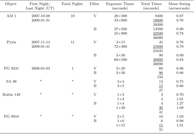
we discover any. Therefore, we always began and ended an observing session with aV frame and alternatedB and V frames in between. A complete list of the observations are listed in Tables A.1 and A.2 in Appendix A. Table 2.2 summarizes the observations.
We operated SOI remotely in Chapel Hill using the Constance and Leonard Goodman
Remote Observing Room (Cecil & Crain 2004, though the facility is now located in Chapman
Hall). On-site telescope operators controlled SOAR under the direction of the observers via
videoconferencing.
In addition to the target clusters, we observed standard stars (or simply “standards”) from
the Landolt (1992) catalog on nights deemed photometric. I determined photometric quality
nights using available weather and satellite data and consultation with the on-site operators.
However, an on-site assessment of photometric conditions is notoriously unreliable. Upper
1
Table 2.2. Summary of observations
Object First Night/ Total Nights Filter Exposure Times Total Times Mean Seeing
Last Night (UT) (seconds) (seconds) (arcseconds)
AM 1 2007-10-08 10 V 28×300 8400 0.87
2009-01-31 33×600 19800 0.76
28200
B 27×500 13500 0.90
25×900 22500 0.78
36000
Pyxis 2007-11-14 11 V 3×15 45 0.76
2009-01-31 72×300 21600 0.79
21645
B 3×30 90 0.89
60×500 30000 0.84
30090
PG 0231 2008-01-03 1 V 3×20 60 0.86
B 3×30 90 0.86
150
SA 98 " " V 3×4 12 0.75
B 3×5 15 0.86
27
Rubin 149 " " V 1×3 3 0.70
1×4 4 1.01
B 1×4 4 1.27
1×30 30 1.08
41
PG 0918 " " V 2×5 10 1.03
B 1×6 6 0.98
1×15 15 1.01
31
atmosphere cirrus clouds are invisible to the unaided eye and can creep in at any point
during the night. The following quote from John Irwin (1952) summarizes the observer’s
frustration.
One might ask: “How clear a sky?” The answer is: “Just as clear as possible-the
best is none too good.” The photocell can “see” and respond to thin cirrus clouds
long before they become apparent to the naked eye. Such clouds are worse than
a nuisance; once they have intruded themselves into the observations their effects
are subtly injurious to the scientific interpretation and are difficult to eradicate.
At the Goethe Link Observatory we call such clouds “photoelectric poison.”
True photometric conditions are most reliably verified post analysis (more details about
this in Chapter 4). Therefore we observed standards on multiple nights until we were
confi-dent we had a truly photometric night. This turned out to be the night of 2008-01-04. Table
2.1 lists the standards observed that night.
2.2 Data Reduction
Image processing refers to the methods of removing the systematic effects of the
instru-ments from the images. Such systematic effects include a bias offset introduced to the analog
to digital converter (ADC) that prevents it from reading a negative number as well as
imper-fections in the optical train, most commonly dust or scratches on the mirrors, that distort
the final image.
I processed the data using the Image Reduction and Analysis Facility (IRAF2, Tody
1993, and references therein). IRAF is an operating environment tailored for Flexible Image
Transport Standard (FITS, Pence et al. 2010) data files commonly used in astronomical
2IRAF is distributed by the National Optical Astronomy Observatories, which are operated by the
applications. It consists of a collection of tasks (or programs) grouped into packages. Each
task receives input from the user through parameters. In this section, all words in the
typeset font refer to IRAF tasks. Typeset words connected by a period refer a parameter
of a task For example, ccdproc.statsub refers to the statsub parameter of the ccdproc
task.
2.2.1 Calibration
The following is a summary of the calibration process based on IRAF CCD documentation
by Massey (1997) to which I refer the reader for details about the tasks below.
Bias Subtraction
In order to correct for the CCD pixel to pixel bias variations, we acquired a sequence
of 10–20 bias (also called zero due to their exposure time) frames at the beginning of each
observing run, which zerocombine combined into a single, averaged image. In order to
account for cosmic rays infiltrating the images, all combination algorithms for the bias and
flat frames discussed below had therejectparameter set tominmax. This master bias frame
was subsequently subtracted from all the images using ccdprocess.
Flat Field Correction
Broadly speaking, flat fielding refers to the process of removing imperfections in the
optics train that cause distortions in the final image and pixel-to-pixel variations in detective
quantum efficiency (DQE). The idea is to have the telescope image a uniformly illuminated
area with an exposure sufficient to provide enough signal to be clearly distinguished from
the background while also not saturating the CCD.
There are two methods for obtaining flat field images (“flats”). The first involves mounting
a screen on the dome and illuminating it with one or more lamps. The telescope then images
the screen to obtain what are commonly called “dome flats”. The advantage of this technique
is that the uniformly illuminated, featureless field free of extraneous signal. However, dome
flats in short wavelength filters, such asB, suffer a lower SNR due to the comparative lack of flux of blue light from the lamp. In principle, this could be addressed with longer exposure
times at the risk of greater hits by cosmic rays.
Incandescent lamps are relatively faint in blue, broadband filters due to the steep drop
off in the blackbody spectrum as wavelength decreases past the effective temperature of
the lamp. Solutions include using incandescent lamps with a hotter effective temperature
and fluorescent bulbs made with gasses with strong blue emission lines. The temperatures
required of the filament to produce such a blue spectrum make incandescent bulbs expensive
and short lived, and fluorescent bulbs only approximate a continuous spectrum with a dense
blanket of emission lines making them less than ideal for broadband filters.
The alternative is to image the sky itself during twilight. The daytime sky is actually
violet, but we perceive it as blue because are eyes are less sensitive to violet wavelengths
(Smith 2005). However, the sky is far too bright to image during the day with a four meter
class telescope. Therefore, we began imaging the flats as soon as the sun set, starting with
the shortest wavelength filter and working our way redward as the sky turns from blue to
red.
Because SOI has a 16 bit ADC, its gain is set such that ADC saturation occurs before
physical the detector’s response becomes non-linear (somewhat near to, but less than, the
point of physical saturation). Saturated pixels have a value of 65,535 counts; the maximum
value of an unsigned 16 bit integer. To reduce the risk of high transparency regions of the
image saturating, we obtained flat field images with median levels less than half that value,
or between 20,000 and 30,000 counts per pixel. We insisted on acquiring enough flats such
that the sum of the median levels of all the individual flats exceed 100,000 counts (typically
A complication that arises when the shutter transfer time, the time it takes for the shutter
to open and close, becomes significant compared to the total exposure time. For example, in
an iris style shutter, pixels first illuminated as the shutter open acquire more signal creating
a gradient on the flat field image that artificially diminishes signal upon application to the
science frames. SOI has a “focal-plane” style shutter, a two curtain system each of which
sweeps across the chip in the same direction, with a 60 millisecond transfer time. This
design purposely minimizes the effects of extra illumination as the first pixels exposed by the
opening curtain are also the first to be blocked by the closing curtain. To limit the maximum
illumination variation to 0.5%, I insisted on a minimum exposure time of four seconds.
Light from stars dominating over the sky brightness is a risk with sky flats. When
imaging the sky, photons from stars and galaxies reach the detector, but their signal tends
to be weak compared to the much brighter sky. As the sky darkens during the flat acquisition
process, stellar light images become significant compared to the sky leading to artifacts in
the flats that could corrupt the final science frames unless accounted for. To correct for this
the telescope operators slightly changed the telescope’s position between sky exposures, a
process called “dithering”. Dithering causes whatever star light that appears in the flat images
to appear in different locations from frame to frame. The flat field processing algorithms,
flatcombine, assumes patterns that change position from frame to frame are stars and
removes them during construction of the final flat image. We used sky flats exclusively during
this campaign, however, dome flats were often acquired each night to serve as backups.
The flat field images were bias subtracted using ccdprocesswith the ccdproc.zero
pa-rameter set to the master bias frame constructed previously. These images were then
com-bined into a single, averaged image for each filter using flatcombine which works similarly
to zerocombine but is designed to identify and filter out star light provided the telescope
position changed from exposure to exposure.
Finally, I bias subtracted and flat field corrected the science frames using ccdprocess