i
IMPLEMENTATION OF MULTIVARIATE ARTIFICIAL NEURAL NETWORKS COUPLED WITH GENETIC ALGORITHMS FOR THE MULTI-OBJECTIVE PROPERTY PREDICTION AND OPTIMIZATION OF EMULSION POLYMERS
A Thesis presented to
the Faculty of California Polytechnic State University, San Luis Obispo
In Partial Fulfillment
of the Requirements for the Degree
Master of Science in Polymers and Coatings Science
by David Chisholm
iii
COMMITTEE MEMBERSHIP
TITLE: Implementation of Multivariate Artificial Neural Networks Coupled with Genetic Algorithms for the Multi-Objective Property Prediction and Optimization of Emulsion Polymers
AUTHOR: David Chisholm
DATE SUBMITTED: June 2019
COMMITTEE CHAIR: Erik Sapper, Ph.D.
Assistant Professor of Chemistry and Biochemistry
COMMITTEE MEMBER: Raymond Fernando, Ph.D.
Director, Western Coatings Technology Center
COMMITTEE MEMBER: Gregory Williams, Ph.D.
iv ABSTRACT
Implementation of Multivariate Artificial Neural Networks Coupled with Genetic Algorithms for the Multi-Objective Property Prediction and Optimization of Emulsion
Polymers David Chisholm
Machine learning has been gaining popularity over the past few decades as computers have become more advanced1. On a fundamental level, machine learning
consists of the use of computerized statistical methods to analyze data and discover trends that may not have been obvious or otherwise observable previously. These trends can then be used to make predictions on new data and explore entirely new design spaces. Methods vary from simple linear regression to highly complex neural networks, but the end goal is similar. The application of these methods to material property prediction and new material discovery has been of high interest as many researchers have begun using the structure-property relationships of materials in conjunction with computational modeling to discover new materials with novel chemical and physical properties2-8.
One such class of materials is that of emulsion polymers, which are heavily used in the coatings industry as they serve as the binder in many waterborne coating systems9-10.
v
vi
ACKNOWLEDGMENTS
I would like to acknowledge and thank my advisor, Dr. Erik Sapper for his support throughout my academic career at Cal Poly as well as during my thesis project work. He encouraged me to work independently and as a result I learned a great deal about programming and how to implement machine learning methods in polymer research.
vii
TABLE OF CONTENTS
Page
LIST OF TABLES ... x.
LIST OF FIGURES ... xii.
CHAPTER 1. INTRODUCTION ... 1
1.1. Machine Learning Methods ... 1
1.1.1. Regression Modeling ... 1
1.1.2. Classification Modeling ... 3
1.1.3. Artificial Neural Network Modeling ... 4
1.1.4. Genetic Algorithms ... 7
1.2. Emulsions ... 9
1.2.1. Surfactants ... 9
1.2.2. Emulsion Stabilization ... 12
1.2.3. Polymerizable Surfactants ... 16
1.3. Emulsion Polymers ... 19
1.3.1. Emulsion Polymerization ... 19
1.3.2. Copolymerization ... 21
1.4. Objectives ... 26
2. EXPERIMENTAL METHODS ... 27
2.1. Emulsion Polymer Synthesis ... 27
2.2. Characterization Methods ... 28
viii
2.2.2. Thermal Properties ... 28
2.3. Test Methods ... 30
2.3.1. Cross-Hatch Adhesion ... 30
2.3.2. Accelerated Dirt Pick-Up Resistance ... 31
2.3.3. Hot Tire Pick-Up Resistance ... 32
2.3.4. Pendulum Hardness ... 33
2.4. Computational Methods ... 34
2.4.1. Data Preparation and Processing ... 34
2.4.2. Artificial Neural Networks and Training ... 34
3. RESULTS AND DISCUSSION ... 37
3.1. Initial Resin Synthesis ... 37
3.2. Computer Modeling ... ... 44
3.2.1. Artificial Neural Network Performance ... 44
3.2.2. Genetic Algorithm Development ... 46
3.3. Neural Network and Genetic Algorithm Prediction Evaluation ... 49
3.3.1. Neural Network Prediction Evaluation ... 49
3.3.2. Genetic Algorithm Prediction Evaluation ... 51
3.4. Neural Network Improvements ... 54
3.4.1. Neural Network Retraining ... 54
3.4.2. Neural Network Prediction Validation ... 55
3.5. Graphical User Interface (GUI) ... 60
3.6. Resin Incorporation into Coatings ... 63
ix
x
LIST OF TABLES
Table Page 1. Hot Tire Pick-Up Resistance Rating Scale ... 33 2. List of Categorical and Continuous Input Variables ... 34 3. List of Categorical and Continuous Output Variables ... 35 4. Resin Recipes’ Adjusted Factors for the First DOE, All Loadings are
Weight Percentages Based on the Total Monomer Loading ... 38 5. Resin Property Data for Continuous Variables ... 39 6. Resin Property Data for Categorical Variables ... 40 7. Final Prediction Errors and Accuracies of the Artificial Neural Networks
Trained on the First DOE Data Set ... 45 8. Polymer Recipes Used to Evaluate the Performance of the Neural
Networks, All Loadings are with Respect to Total Monomer ... 49 9. Predicted and Measured Values for the Properties of the Validation
Batches ... 50 10.Desired Performance Criteria for Each of the Runs of the Genetic
Algorithm ... 51 11.Polymer Recipes Found by the Genetic Algorithm to Have the Highest
Fitness Scores, All Loadings Shown are with Respect to Total Monomer . 52 12.Predicted and Measured Values for the Properties of the Validation
Batches with the Predicted Fitness Scores and the Actual Fitness Scores .. 53 13.Final Prediction Errors and Accuracies of the Neural Networks Trained
xi
14.Second Set of Polymer Recipes Used to Evaluate the Performance of
the Neural networks, All Loadings are with Respect to Total Monomer .... 56 15.Variations in the Validation Batches Used to Test the Neural Networks’
Capabilities ... ... 57 16.Differences Between Predicted and Measured Values for the P roperties
of the Validation Batches ... 57 17.Average Error of Predictions Compared to the Average Model Errors ... 58 18.Final Prediction Errors and Accuracies of the Neural Networks Trained
Using the First DOE Data Set and All Validation Batches ... 59 19.Adhesion Performance of 30% Volume Solids Paints Formulated at
xii
LIST OF FIGURES
Figure Page 1. Simple Linear (Top) and Polynomial Regression (Bottom) Example
Graphs ... 2
2. Conversion of a List of Categorical Variables to a List of Dummy Variables ... 3
3. General Structure of an Artificial Neural Network ... 5
4. Example of a Weight Vector Within a Neural Network ... 6
5. Schematic Representation of How a Genetic Algorithm Sequentially Determines the Correct Sequence of Genes ... 8
6. Oil-in-Water Emulsion Stabilized by Surfactant Molecules ... 9
7. Surfactant in Water Just Below (Left) and Above (Right) its CMC ... 10
8. Chemical Structure and Shape of Sodium Dodecyl Sulfate ... 11
9. Schematic Representation of the Potential Distribution as a Function of Distance from the Surface of a Charged Particle ... 13
10.Schematic Representation of DLVO Interactions; the Sum of the Attractive and Repulsive Potential Energy Curves Result in the Total Potential Energy Curve ... 14
11.Example Structure of a Non-Ionic Surfactant ... 15
12.Example Structure of a Surfactant That Would Exhibit Electrostatic and Steric Stabilization ... 16
13.Surfactant Leaching of a Painted Wall ... 17
xiii
15.Common Acrylic Monomers Used in Emulsion Polymerization ... 20
16.Pictorial Representations of Heterogeneous and Homogeneous Nucleation in the First Stage of Emulsion Polymerization ... 21
17.Pictorial Representation of the Particle Growth Stage of Emulsion Polymerization ... 22
18.Relevant Reactions and Their Rates Needed to Determine the Monomer Reactivity Ratios of a Given Pair of Monomers ... 24
19.Summarization of Reactivity ratios of Terminal and Penultimate Models .. 25
20.Cross-Hatch Adhesion Test Substrate Appearance After Cutting the Film . 30
21.Cross-Hatch Adhesion Rating Scale from ASTM D3359-97 ... 30
22.Hot Tire Pick-Up Resistance Press Set to 22mm with a Sample Inside ... 32
23.Example Form of a ReLU Activation Function ... 36
24.Chemical Structure of EDTA ... 42
25.Pictorial Representation of How k-Fold Cross-Validation Splits a Dataset of Six Observations into Three Folds and Configures the Data into Training and Test Sets ... 44
26.Continuous Neural Network Property Prediction Errors (Top) and Categorical Neural Networks Property Prediction Accuracies (Bottom) As a Function of Folds ... 45
27.Example of How Recipes Would be Scored by the Fitness Function According to Specified Criteria ... 47
xiv
29.Training Results for the Third Training of the Neural Networks Using All of the Collected Data from the First DOE and All Validation
Batches ... 59 30.Home Screen of the GUI Used to Predict Polymer Properties and Recipes 60 31.Property Predictor Window (Left) with Input Recipe Components and
Predictions Window (Right) with the Corresponding Properties ... 61 32.Recipe Predictor Window (Left) with Input Property Criteria and
1 1. Introduction
1.1. Machine Learning Methods
1.1.1. Regression Modeling
Machine learning is a catch-all term used to describe the use of statistical techniques and methods on computers to model relationships between variables that are known and unknown, the two main types of machine learning being unsupervised and supervised. In unsupervised machine learning, the output variables are not known, with the goal being to model the structure present in a given set of data. Conversely, in supervised machine learning, the types of output variables and what they should be are known11.
In all supervised machine learning schemes, the input and output variable sets that will be modeled are split into training sets and test sets. The size of the training and test sets determines how well the model can learn12, with an 80-20 split being the common
practice for most models. The model is first trained on the training input and provided output variables before its accuracy is tested against the test set, which is meant to mimic new data that has not been seen by the model13. The ultimate goal of this supervised
learning scheme is to develop a function that best describes the relationship between the input variables and output variables. The type of function that is fit to the data can be varied with the simplest form being a straight line.
For simple linear regression14 using the least squares method, the aim is to find a
2
𝑆 = ∑𝑛𝑖=1∆𝑛2 (1)
∆ = (𝑦 − 𝑦̂) (2)
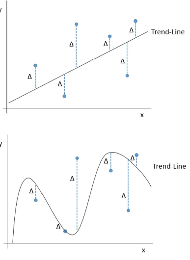
A simplified example of a linear regression of a data set with only one input and one output variable can be seen in the top graph of Figure 1. While this example has only one input variable, the least squares regression method is not limited solely to systems that have only one input variable15. When there are multiple input variables, instead of having
only one summation to consider, there is one summation for every input variable. The resultant sum of these sums is then what is minimized instead of the single summation.
3
In addition to linear regression using straight lines, data can also be modeled using curved lines such as polynomials as shown in the bottom graph of Figure 1, where the data is modeled using a three degree polynomial. Though the line is curved, the concept remains the same: the distance between the predicted and actual values is minimized to give the best fitting line. While these methods are useful for modeling trends in output data that is numerical, they cannot model trends in data that is categorical.
1.1.2. Classification Modeling
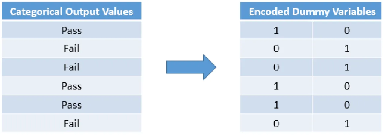
Classification models differ from regression models in that the output variables they predict are categorical in nature and not numerical. These models tend to be more complex than regression models, as the categorical variables are represented by vectors of ones and zeros called dummy variables16. For instance, trying to predict whether or not a given
polymer will be able to form a film at room temperature would be a classification problem and the schematic in Figure 2 illustrates how a small list of outputs from that test with two unique values would be transformed into dummy variables.
4
Once the data is properly encoded, the implementation of algorithms such as decision tree and support vector machine can be done, which essentially determine how to sort the data into the output categories based on the input variables.
1.1.3. Artificial Neural Network Modeling
Artificial neural networks (ANNs) are among the more advanced machine learning methods, even placed in their own class of machine learning named deep learning. This technique can be either supervised or unsupervised and these neural networks can take any number of categorical and continuous input variables and utilize them to predict either categorical17 outputs using classification or continuous18 outputs using regression, though
both types of outputs cannot be modelled in the same neural network.
Neural networks are highly useful when the precise nature of the relationship between variables is either unknown or not desired to be known19, essentially acting as a
5
Figure 3. General Structure of an Artificial Neural Network
The general structure of an artificial network, meant to mimic that of the human brain, is shown in Figure 3, where the model has a layer of input neurons, one or more hidden layers, and lastly an output layer. The number of hidden layers and the number of neurons, also known as nodes, in each of those layers is a matter of hyperparameter optimization in any given system. Too many hidden layers can result in overfitting20, where
6
variance and would therefore be difficult to model. If the variance of the model is too high without having a lot of data points to fill in the gaps between points, however, then local minima and maxima could be missed.
Artificial neural networks are trained in a similar fashion to that of simpler models : the data set is split into training and test sets, the model learns correlations based on the training set, and then the model’s performance is tested on the test set. The major difference between neural networks and simpler models is how the training step is done and the procedure used to do this is known as the optimization algorithm21. There are several
different optimization algorithms, with gradient descent22 being the simplest and therefore
widely utilized. In this scheme, the goal is to minimize the loss function by adjusting the weights applied to the nodes within the network. This is accomplished in a process called backpropagation23.
Figure 4. Example of a Weight Vector Within a Neural Network23
7
been completed, the networks can then be evaluated using the test set and then used to predict new outcomes in the same manner as other machine learning methods.
The advantage of using artificial neural networks over other machine learning models is that they are highly accurate models that essentially encompass all of the other machine learning models. Neural networks tend to require more data than other models but are able to handle many input and output variables, both categorical and continuous, more efficiently than other models. The more input and output variables that are being modeled, however, the longer the training and optimization of the networks will take and the more computationally expensive the overall process will be.
1.1.4. Genetic Algorithms
Similar to the backpropagation algorithms used in training neural networks, genetic algorithms are tools used for the targeted optimization of specific variables with constraints based on the theories of natural selection and evolution24. In most genetic algorithms, the
first generation or set of genes is randomly selected from a larger set of genes making the parent. This parent set is then evaluated in a fitness function and if the fitness is less than the defined optimal fitness, the genes will be mutated. The way in which the mutation is done can be varied depending on the nature of the problem25, but essentially one of the
8
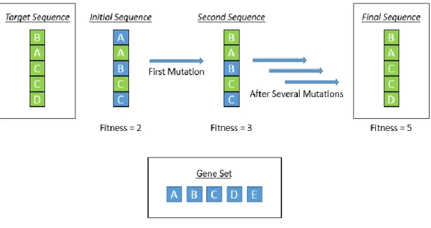
Figure 5. Schematic Representation of How a Genetic Algorithm Sequentially Determines
the Correct Sequence of Genes
In the example above, both the order and identity of the letters matter and as such the first sequence has a fitness score of two and not three, even though it has two C’s and a B like the target sequence. If only the identity of the letters mattered and not the order, then the fitness score of the first set of genes would have been four instead of two. Every genetic algorithm is different and how the genes are selected, mutated, and finally evaluated in the fitness function is highly important and determines how efficiently the algorithm will perform26.
9 1.2. Emulsions
1.2.1. Surfactants
Emulsions are essentially dispersions of one phase of material in a larger continuous phase of another, i.e. hexane in water and as mentioned previously, the emulsions in this work consist of polymer particles dispersed in aqueous media. These systems differ greatly from solutions, as the phases in these mixtures are completely distinct from one another and are not homogeneously mixed as they are in solution. If desired, the two could be separated rather easily, whereas this is not the case with solutions. Depending on the hydrophilicity of the dispersed polymer particles, some amount of water will be able to enter the particles, however, the vast majority of the water remains outside of the particles27. As the two phases do not want to mix with one another due to the polarity
differences between them, emulsions are inherently unstable and will eventually separate into two different phases.
Figure 6. Oil-in-Water Emulsion Stabilized by Surfactant Molecules
10
molecules having both hydrophilic and hydrophobic portions which have been shown to preferentially position themselves at interfaces between different phases of materials28-30.
While at these interfaces, the free energy of the surfactants is minimized as both portions of the molecule have favorable interactions as they are surrounded by similar species. These surfactants are not locked in place, however, having the ability to move across the emulsified droplet surface and even migrate from one emulsion droplet to another neighboring droplet.
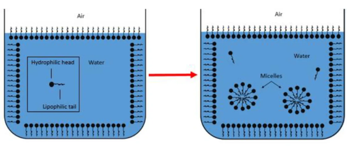
Figure 7. Surfactant in Water Just Below (Left) and Above (Right) its CMC
Surfactants do not form micelles immediately upon addition to a liquid, however, and some do not form micelles at all. In order for a surfactant to form micelles in a given system, its concentration in that system needs to be above its critical micellar concentration, defined as the concentration above which a surfactant will begin to form micelles31. When
11
molecules. Adding additional surfactant above this point will result in micelle formation in the liquid phase in the form of spherical aggregates of surfactant molecules. For surfactants added to water, or another polar solvent, the hydrophobic tails will face toward one another, with the hydrophilic portion pointed out into the water phase. For a surfactant added to a non-polar solvent, the orientation of the surfactant would be reversed, having the hydrophilic portion facing inwards and the hydrophobic portion facing out into the solvent phase.
Conventional surfactants used for the stability of oil-in-water emulsions consist of a hydrophilic head attached to a hydrophobic tail, usually an alkyl chain. The chemical structure of surfactants can be highly variant as the major requirement for a molecule to act as a surfactant is for it to be amphiphilic, having both a hydrophilic portion and a lipophilic portion. Not all molecules that are amphiphilic will make good emulsifying agents in all systems, however, as the hydrophile-lipophile balance (HLB) value and the surfactant number (Ns) of each candidate need to be considered32.
The HLB value indicates the relative hydrophilicity and conversely the lipophilicity of a given surfactant whereas the surfactant number indicates what type of shape the surfactant molecule adopts. Sodium dodecyl sulfate, for instance, as shown in Figure 8, has a higher HLB value and it adopts a cone-like shape, making it better suited to stabilize spherical oil-in-water emulsions.
12
Surfactants that have higher HLB values tend to have higher critical micellar concentrations as these are more hydrophilic and therefore a higher concentration of the surfactant molecules can remain in the water phase before needing to collapse into micelles to lower their free energy. The higher the hydrophobicity of a given surfactant, the lower the concentration of surfactant needed to form micelles in water33, whereas the reverse is
true in non-polar solvents like hexane or xylene. Regardless of which surfactant is selected for any given system, the main modes of stabilization they can provide to an emulsion include electrostatic and steric stabilization.
1.2.2. Emulsion Stabilization
The use of ionic surfactants, like sodium dodecyl sulfate, would contribute to electrostatic stabilization34 whereas non-ionic surfactants with long hydrophilic chains
would contribute to steric stabilization35. When the ionic surfactants are added to a system
of dispersed polymer particles, the surfactants’ hydrophobic tails are able to adsorb onto the polymer particle surface, adding a layer of charges to the particles, dubbed the Stern Layer36. This layer of charges can either be positive or negative, depending on the
13
Diffuse Layers is known as the Electric Double Layer and this double layer gives the particles an overall effective charge otherwise known as the zeta potential.
Figure 9. Schematic Representation of the Potential Distribution as a Function of Distance
from the Surface of a Charged Particle37
When particles that have like charges approach one another there is an electrostatic repulsive force generated which keeps the particles apart, in accordance with DLVO Theory38. There is an attractive force due to Hamaker attractions which gets larger as the
14
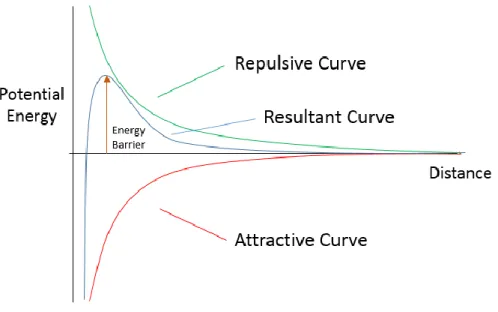
Figure 10. Schematic Representation of DLVO Interactions; the Sum of the Attractive and
Repulsive Potential Energy Curves Result in the Total Potential Energy Curve
The stabilization of these particles can be reduced significantly, however, if ions from salts such as sodium chloride are added to the system39. When these ions are added,
the thickness of the electric double layer of the particles gets reduced, resulting in a decrease in the zeta potential of the particles. Since the particles do not have as high a charge as they had previously, the magnitude of the electrostatic force that prevents them from coming together is proportionally lowered, lowering the energy barrier and making it easier for the particles to agglomerate. The concentration of ions needed to completely destabilize a given emulsion or suspension of particles is defined as the critical coagulation concentration40. At this concentration of ions, the zeta potential of the particles is
essentially lowered to zero, resulting in rapid agglomeration of the particles due to their being no energy barrier and ultimately complete separation of the two phases. In addition to concentration of ions, the charge of those ions plays a large role as well41. Ions with
15
concentration than ions with a charge of +1. In certain situations this is very useful, i.e. cleaning murky water to make it safe to drink42, however, this destabilization is not
normally desired in the case of polymer emulsions.
Figure 11. Example Structure of a Non-Ionic Surfactant
Non-ionic surfactants with water soluble chains of ethylene oxide units, such as the one shown in Figure 11, are able to avoid this ion-induced destabilization because they stabilize emulsions via an entropic mechanism. When the ethylene oxide chains are pointed out into the water phase, the chains have a large degree of conformational entropy, meaning the chains can take on many different conformations in the water phase without being hindered43. If two particles that have these surfactants come close to one another, the total
16
Figure 12. Example Structure of a Surfactant that Would Exhibit Electrostatic and Steric
Stabilization
A common practice is to use both non-ionic and ionic surfactants together in the same emulsion system to provide better stabilization45 by utilizing both stabilization
mechanisms. Surfactants are also commercially available with structures similar to the one shown in Figure 12 that combine the two stabilization mechanisms into one molecule by having a hydrophobic group that is a chain of ethylene oxide units capped with an ionic group. This class of surfactants has the advantage of exhibiting both stabilization mechanisms in one molecule and although they are still susceptible to lessened stabilization if more electrolytes are added to the system, the added electrolyte ions are less likely to cause complete destabilization of the dispersion.
1.2.3. Polymerizable Surfactants
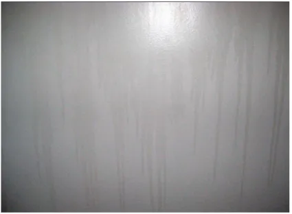
17 Figure 13. Surfactant Leaching of a Painted Wall46
These issues can be overcome, however, through the use of surfactants that are polymerizable instead of conventional surfactants, an example structure of which is given in Figure 14. Polymerizable surfactants used for the stabilization of emulsion polymers are molecules that have reactive groups somewhere in the hydrophobic portion of the molecule that can participate in the radical polymerization reaction.
Figure 14. Example Structure of a Polymerizable Surfactant
Since these surfactants have unsaturated double bonds, they are able to react with the growing polymer chain radicals and as a result these surfactants will end up in the polymer backbone47, assuming they have comparable reactivity to that of the monomers in
18
19 1.3. Emulsion Polymers
1.3.1. Emulsion Polymerization
Emulsion polymers can be synthesized in a number of different ways with free-radical emulsion polymerization being the predominant method. This method’s mechanism was outlined by Harkins48 in the 1940s and its full mechanism is still the subject of some
debate, though it’s widely accepted that the reaction proceeds through three major stages: nucleation, particle growth, and finally the consumption of monomer. The vast majority of emulsion polymerizations are conducted in water, with monomer being the dispersed phase, as their end applications, i.e., paint resins, require them to be water-based systems. The major components needed for these emulsion polymerizations include monomer, surfactant, and a water-soluble initiator. Other components can be added to aid in processing, such as defoamer to reduce foam formation or chain transfer agents for molecular weight control49-50, but they are not necessarily required.
20
also be used, but monomers that react with water should be avoided, as they can destabilize the emulsion or even prevent it from forming at all.
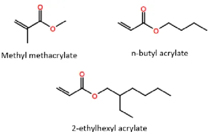
Figure 15. Common Acrylic Monomers Used in Emulsion Polymerization
The first stage of free-radical emulsion polymerization, particle nucleation, can begin by either homogeneous nucleation or heterogeneous nucleation. In homogeneous nucleation, initiator radicals in the water phase react with the small amount of monomer molecules that are present51. Once the growing chain becomes too large to be soluble in
21
different, the end result of both mechanisms is the same for both types of nucleation, illustrated in Figure 16.
Figure 16. Pictorial Representations of Heterogeneous and Homogeneous Nucleation in
the First Stage of Emulsion Polymerization
Once all of the surfactant molecules in the system are in micelles and there is none left to form new micelles, the second stage, particle growth, begins. As depicted in Figure 17, during this stage, the total number of particles within the system is fixed, meaning no
22
Figure 17. Pictorial Representation of the Particle Growth Stage of Emulsion
Polymerization
As the polymer particles increase in size, the monomer droplet micelles get depleted and the surfactant molecules that were stabilizing those monomer droplets migrate into the polymer particle micelles. The final stage of the polymerization begins when all of the monomer droplet micelles have been depleted and all surfactant molecules have migrated to polymer particles.
23 1.3.2. Copolymerization
Nearly all emulsion polymers are copolymers, meaning their composition includes more than one monomer species. Meeting desired performance attributes for coatings applications using only one monomer is highly unlikely and therefore multiple monomers are incorporated to adjust the polymers’ chemical and physical properties such as the glass transition temperature (Tg). An emulsion polymer intended for use in a coating to be
applied at room temperature, for example, would need to have a glass transition temperature in the range of 0-5°C to minimize the amount of coalescent needed for the paint to form a cohesive film. The Tg of any copolymer can be calculated using the Fox
Equation, equation 3, where Tg is the glass transition temperature of the copolymer, W1
and W2 are the weight fractions of each of the monomers, and Tg1 and Tg2 are the glass
transition temperatures of the homopolymers of the respective monomers.
1
𝑇𝑔
=
𝑊1
𝑇𝑔1
+
𝑊2
𝑇𝑔2
(3)
24
Figure 18. Relevant Reactions and Their Rates Needed to Determine the Monomer
Reactivity Ratios of a Given Pair of Monomers
The monomer reactivity ratio53 is defined as the ratio of the rate of monomer one
(M1) addition to a monomer one radical (M1*) divided by the rate of monomer two (M2) addition to a monomer one radical (M1*). If a monomer reacts more often with the radical analogue of itself than that of the other monomer radical, then it would have a high reactivity ratio. This would not be an ideal scenario for a random distribution of monomers in a copolymer, however, as the monomers have a preference over which radical they add to. In order for a copolymer to have a random composition, there needs to be little to no preference in monomer addition.
These equations are based on the terminal model and this model ignores the influence of neighboring monomers on the reactivity of the radical, stating that the reactivity of a radical is independent of what that radical is attached to54. This is an
25
Figure 19. Summarization of Reactivity Ratios of Terminal and Penultimate Models54
26 1.4. Objectives
27 2. Experimental Methods
2.1. Emulsion Polymer Synthesis
All of the polymers in this study were synthesized using a proprietary starve-fed emulsion polymerization procedure, allowing for controlled particle growth as well as lower polydispersity of particle sizes55. Sometimes referred to as semi-continuous batch
28 2.2. Characterization Methods
2.2.1. Quality Check (QC) Properties
Polymer physical properties were evaluated including: density, particle size, weight percent solids, and pH. Density was determined using a pycnometer and pH was measured using a two-point calibrated pH probe. Polymer pH was measured before and after correction with ammonia to a range of 8.5-9. Weight percent solids for the polymers was measured using a solids analyzer. Wet samples were put into a tray and an initial mass was taken. The samples were then heated from 60°C to 150°C and held at 150°C until the mass of the tray no longer changed. The percent solids, then, were expressed as a percentage of final mass divided by initial mass. Particle size was measured via dynamic light scattering using a Nano-S Zetasizer from Malvern with a scattering angle of 173°.
2.2.2. Thermal Properties
Differential scanning calorimetry (DSC) was conducted on the emulsion polymers using a DSC 214 Polyma® from Netzsch to determine their glass transition temperatures. Drawdowns of the polymers were made using a standard 3-mil drawdown bar on Leneta release charts and allowed to dry for at least one day before testing. Squares were cut from the dried films and tested in the DSC. To mitigate the effects of water and erase the sample thermal history56-57, all samples were annealed at 105°C for two minutes before the testing
29
30 2.3. Test Methods
2.3.1. Cross-Hatch Adhesion
Cross-hatch adhesion was conducting according to a modified version of ASTM D3359-9758. The emulsion polymers were applied as-is using a natural spread rate, onto a
block of unprepared, smooth concrete using a foam brush. Adhesion was then evaluated on these films in the following manner, at times of one day and seven days after the films were applied.
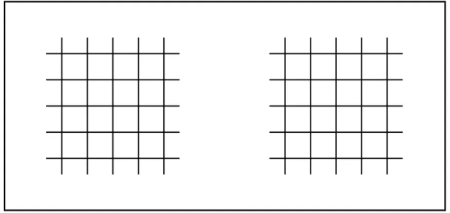
Figure 20. Cross-Hatch Adhesion Test Substrate Appearance after Cutting the Film
31
Following this, pieces of adhesion tape were stuck to both sets of squares and force was applied to ensure the tape was indeed stuck to all of the individual squares. The tape was then removed in a swift upward motion. Both wet and dry adhesion were rated based on how much of the coating was removed according to the scale shown in Figure 21.
Figure 21. Cross-Hatch Adhesion Rating Scale from ASTM D3359-9758
2.3.2. Accelerated Dirt Pick-Up Resistance
32
performance was rated on a 0-5 scale, with a score of zero being very dirty and a score of five having very little to no dirt.
2.3.3. Hot Tire Pick-Up Resistance
Hot tire pick-up resistance of the resins was measured one day and seven days after application onto 3x3” concrete tiles. The tiles were split in two after being applied in the same manner as the samples for adhesion and accelerated dirt-pick up resistance. A rectangular piece of a tire was dipped in water and then placed on top of the concrete tile. The two were then placed into a press which was then depressed to 21mm, measured from the tip of the top vertical bar to the line indicated on the bottom vertical bar, shown in Figure 22.
33
The whole apparatus was then placed in a 65ºC oven for one and a half hours. Following this, the apparatus was removed from the oven and the press was unscrewed to remove the tile and tire. Samples were rated based on how difficult it was to remove the tire from the surface of the coating as well as the condition of the coating after tire removal in accordance with the scale shown in Table 1.
Table 1. Hot Tire Pick-Up Resistance Rating Scale
Surface Condition Rating Scale
No sticking, no imprint, no delamination 10 No sticking, slight imprint, no delamination 9 Slight sticking, slight imprint, no delamination 8 Moderate to slight sticking, slight imprint, no delamination 7 Moderate sticking, slight imprint, no delamination 6 Moderate sticking, moderate imprint, no delamination 5 Moderate sticking, slight imprint, slight delamination 4 Moderate sticking, moderate imprint, slight delamination 3 Severe sticking, moderate imprint, slight delamination 2 Severe sticking, severe imprint, slight delamination 1 Severe sticking, severe imprint, delamination 0
2.3.4. Pendulum Hardness
34 2.4. Computational methods
2.4.1. Data Preparation and Processing
Before the neural networks could be trained on the data set, the input and output variables needed to be scaled and encoded. Recipe variables such as surfactant and adhesion promoter and their respective chemistries were encoded as dummy variables and loading levels were scaled to a 100 scale so that no values were greater than one. This was done to improve the efficiency of the neural networks in predictions as well as training. A complete list of both continuous and categorical input variables is listed in Table 2.
Table 2. List of Categorical and Continuous Input Variables
Variable Variable Type
Surfactant Chemistry Categorical Surfactant Loading Continuous Adhesion Promoter Chemistry Categorical Adhesion Promoter Loading Continuous Bulk Monomer 1 Loading Continuous Bulk Monomer 2 Loading Continuous Acid Monomer Loading Continuous
Theoretical Tg Continuous
Theoretical Weight Percent Solids Continuous
2.4.2. Artificial Neural Networks and Training
35
Table 3. List of categorical and continuous output variables
Property Property Type Property Units/Scales
Percent Recovered Continuous %
Actual Tg Continuous Kelvin
MFFT Continuous Kelvin
Particle Size Continuous Nanometers
Weight % Solids Continuous %
Koenig Hardness Continuous Swings
Pre-emulsion Stability Categorical Pass/Fail
Dry Concrete Adhesion Categorical 0-5, 5 best
Wet Concrete Adhesion Categorical 0-5, 5 best Dirt Pick-up Resistance Categorical 0-5, 5 best Hot Tire Pick-up Resistance Categorical 0-10, 10 best
All modeling and computational work was conducted in Python, using Keras and TensorFlow as the main packages for the neural networks. The continuous properties were all modeled using a single neural network while separate classification networks were trained for each of the categorical properties resulting in a total of six neural networks. All of the neural networks were trained using a modified k-fold strategy in which the data set was split k times into training and test folds and then the models were trained and evaluated sequentially on each of the folds in the data. Optimal model hyperparameters including activation functions, number of hidden layers, number of nodes etc. were determined using a combination of trial and error and grid searching to minimize the amount of error in the model predictions.
For nearly all of the networks, the activation function applied to the weight vectors from the input layer to the hidden layer was ReLU59. ReLU, or rectified linear units, is a
36
Figure 23. Example Form of a ReLU Activation Function59
37 3. Results and Discussion
3.1. Initial Resin Synthesis
As with all neural networks and machine learning models, a data set is needed with which to train and evaluate the model. In order to generate a data set in a systematic way, a standard design of experiments, or DOE60, was conducted by varying adhesion promoter
38
Table 4. Resin Recipes’ Adjusted Factors for the First DOE, All Loadings are Weight Percentages Based on the Total Monomer Loading
Resin Adhesion Promoter
General Chemistry Promoter Loading
Surfactant General Chemistry
1 None 0% Sulfate
2 None 0% Non-ionic
3 None 0% Phosphate
4 Phosphate 1% Sulfate
5 Phosphate 1% Non-ionic
6 Phosphate 1% Phosphate
7 Phosphate 2% Sulfate
8 Phosphate 2% Non-ionic
9 Phosphate 2% Phosphate
10 Ureido 0.5% Sulfate
11 Ureido 0.5% Non-ionic
12 Ureido 0.5% Phosphate
13 Ureido 1% Sulfate
14 Ureido 1% Non-ionic
15 Ureido 1% Phosphate
16 Alkoxysilane 1% Sulfate
17 Alkoxysilane 1% Non-ionic
18 Alkoxysilane 1% Phosphate
19 Alkoxysilane 2% Sulfate
20 Alkoxysilane 2% Non-ionic
21 Alkoxysilane 2% Phosphate
22 Ureido 1% Sulfate
23 Ureido 1% Non-ionic
24 Ureido 1% Phosphate
25 Ureido 2% Sulfate
26 Ureido 2% Non-ionic
27 Ureido 2% Phosphate
39
3.1.1. Resin Physical Properties and Performance
Table 5. Resin Property Data for Continuous Variables
Resin % Recovered Actual
Tg (K) MFFT (K) PS (nm)
Wt % Solids
Hardness (swings)
1 86.4 284.8 278.2 136 49.14 15
2 87.6 284.4 279.8 157 51.19 14
3 90.2 285.3 283.7 143 48.89 28
4 87.4 291.8 281.2 149 49.30 19
5 85.8 290.9 281.8 152 51.39 16
6 92.2 292.3 282.6 135 47.85 21
7 92.4 286.6 280.4 137 50.01 17
8 89.2 287.4 280.8 142 48.83 13
9 93.2 289.0 281.6 140 48.74 20
10 88.0 290.6 281.4 155 49.88 16
11 88.1 287.8 281.0 156 49.98 13
12 90.7 289.6 282.6 160 49.96 23
13 82.6 285.6 281.6 137 52.96 19
14 91.6 286.9 281.6 218 49.84 15
15 90.0 288.3 284.0 140 49.50 19
16 88.0 283.6 281.0 142 49.95 20
17 89.1 288.4 281.4 163 50.71 17
18 90.4 288.8 281.2 129 49.74 23
19 90.7 292.7 282.0 140 48.73 22
20 90.2 291.3 282.0 139 48.92 17
21 91.7 292.8 282.0 134 48.02 24
22 86.4 290.0 279.4 147 48.88 16
23 88.4 296.3 279.4 188 48.23 15
24 88.6 294.3 279.4 152 48.87 22
25 73.1 290.9 281.6 191 53.05 17
26 79.4 289.1 281.6 203 49.84 13
40
Table 6. Resin Property Data for Categorical Variables
Resin Pre-Emulsion
Stability Dry Adhesion Wet Adhesion DPUR HTPUR
1 Stable 5 4 0 1
2 Stable 5 4 0 2
3 Stable 4 4 1 2
4 Stable 5 5 0 0
5 Stable 5 5 0 1
6 Stable 5 5 2 0
7 Stable 5 2 0 1
8 Stable 4 2 0 0
9 Stable 5 5 2 0
10 Stable 5 5 0 0
11 Stable 5 5 0 1
12 Stable 5 5 1 0
13 Stable 4 4 0 5
14 Stable 4 2 0 1
15 Stable 2 1 1 0
16 Stable 5 5 0 6
17 Stable 5 5 0 3
18 Stable 5 5 1 8
19 Stable 5 5 0 2
20 Stable 5 4 0 0
21 Stable 5 5 0 6
22 Stable 5 5 0 7
23 Stable 5 5 0 6
24 Stable 5 5 2 2
25 Stable 5 5 0 1
26 Stable 5 5 0 1
27 Unstable NA NA NA NA
41
hydrophilicity of the surfactant. Though it has nearly the same chemistry and structure as the other surfactants, it does have higher solubility in water and as such would not be expected to be as efficient as the other two surfactants at stabilizing emulsions61. Other
batches within this DOE also separated overnight, but upon mixing re-emulsified without issue.
Initially, adhesion was tested on both etched an unetched concrete, however, all samples were able to pass both wet and dry adhesion on etched concrete. For most concrete coatings to adhere to concrete substrates, the concrete needs to be etched with an acid solution such as hydrochloric acid in order to provide a sufficiently rough surface. As the roughness of the concrete’s surface increases, the adhesion of the coating proportionally improves62 as there is more surface area available for the polymer to interact with the
concrete. In addition to providing roughness, etching also increases the porosity of the concrete, allowing for better penetration of the coating into the substrate, also improving the adhesion performance. Since there was no variation in performance observed between samples on etched concrete, it was not pursued, instead opting for adhesion to unetched concrete. Both the dry and wet adhesion ratings recorded in Table 6, then, are adhesion to unprepared, smooth concrete.
42
ethylenediaminetetraacetic acid (EDTA), shown in Figure 24, have been shown to chelate to calcium when deprotonated63-68.
Figure 24. Chemical Structure of EDTA
As calcium chloride is used in the manufacture of concrete69, it is logical to infer
that the carboxylic acid groups in the polymer would be able to chelate to the calcium ions in the concrete, providing some degree of adhesion through those ionic interactions. The phosphate adhesion promoter is meant to do the same, able to chelate to many different types of metals and thereby provide improved adhesion to inorganic substrates. So it stands to reason that the carboxylic acid functional groups would be able to do the same but to a lesser degree as there is only one negative charge to interact with the substrate while the phosphate group has two.
43
weaker because the film will not be able to flex with the tire and therefore will easily delaminate from the substrate when the tire is removed. One way to overcome this is to lower the surface energy of the polymer, which would decrease the attractive forces between the surfaces of the tire and the polymer film70, thereby reducing the likelihood of
44 3.2. Computer Modeling
3.2.1. Artificial Neural Network Performance
Once all of the data had been collected for the first set of resins, the first set of artificial neural networks were trained using a modified k-fold cross-validation method. In normal k-fold cross-validation, a set of data is split into folds and then these folds are used in different combinations to train and evaluate models to test the skill of an overall model as illustrated in Figure 25. In this process, a new model is trained and evaluated at each configuration of the data and then discarded.
Figure 25. Pictorial Representation of How k-Fold Cross-Validation Splits a Dataset of
Six Observations into Three Folds and Configures the Data into Training and Test Sets
45
Table 7. Final Prediction Errors and Accuracies of the Artificial Neural Networks Trained
on the First DOE Data Set
Property Error & Accuracy of
Models’ Predictions
% Recovered ± 2
Actual Tg (K) ± 3
MFFT (K) ± 2
Particle Size (nm) ± 7
Wt % Solids ± 1
Hardness (swings) ± 2
Dry Adhesion 100%
Wet Adhesion 100%
Dirt Pick-Up Resistance 100%
Hot Tire Pick-Up Resistance 100%
Figure 26. Continuous Neural Network Property Prediction Errors (Top) and Categorical
46
Although the errors in predictions for the continuous variables are low and the accuracies of the classifications of categorical variables are high, one major issue with this first data set is that it is not variant in terms of adhesion and dirt pick-up resistance and is therefore biased71. Almost all of the resins had good adhesion and all of the resins had poor
dirt pick-up resistance. After being trained on this skewed data set, the models will likely end up predicting that all future polymer recipes will result in good adhesion and poor dirt pick-up resistance. While this may be the case within the design space of the DOE, it is not likely and this is most definitely not the case for all possible polymer recipes. There are bound to be polymers that have terrible adhesion and polymers that have exceptional dirt pick-up resistance, but the models cannot recognize this as they were not trained on data that reflects this.
3.2.2. Genetic Algorithm Development
47
The fitness function then compared the values in the predicted vector to those in the target vector. Each of the properties were evaluated and given a binary score of either one, if the value met the specified criteria, or zero if the value did not meet the specified criteria. These scores were stored in a vector and the sum of that vector was defined as the fitness score for that recipe. If the fitness score was less than the defined optimal fitness, then the algorithm would mutate the recipe, switching one of the components’ values with a different value, and then the performance values for that recipe would be determined and subsequently evaluated in the fitness function again. This process was done iteratively until an optimal fitness score was reached. An example of how recipes’ performance values would be scored by the fitness function is provided in Figure 27. The first recipe receives a score of two out of ten as only two of the properties meet the fitness criteria while the second recipe receives a score of five out of ten because five of its properties match the fitness criteria defined in the second table.
Figure 27. Example of How Recipes Would be Scored by the Fitness Function According
48
49
3.3. Neural Network and Genetic Algorithm Prediction Evaluation
3.3.1. Neural Network Prediction Evaluation
In order to test the validity of the models’ prediction accuracies and their ability to extrapolate, polymers were synthesized that had recipes intentionally outside of the current design space of the models. While surfactant loading and theoretical glass transition temperature were held constant in the first DOE, these recipe components were deliberately varied in the second round of resins. The full list of recipes for the second set of resins are shown in Table 8 and the predicted properties and experimentally determined properties are shown in Table 9.
Table 8. Polymer Recipes Used to Evaluate the Performance of the Neural Networks, All
Loadings are with Respect to Total Monomer
Validation 1 Validation 2 Validation 3
Surfactant Chemistry Non-ionic Sulfate Non-ionic
Surfactant Loading 1.0% 1.0% 5.0%
Adhesion Promoter Chemistry Alkoxysilane Alkoxysilane Alkoxysilane
Adhesion Promoter Loading 0.5% 0.5% 1.0%
Bulk Monomer 1 Loading 52.274% 55.8% 51.898%
Bulk Monomer 2 Loading 46.226% 42.7% 46.102%
Acid Monomer Loading 1.0% 1.0% 1.0%
Theoretical Tg 273.15 268.15 273.15
50
Table 9. Predicted and Measured Values for the Properties of the Validation Batches
Validation 1 Validation 2 Validation 3
Predicted Values Measured Values Predicted Values Measured Values Predicted Values Measured Values
% Recovered (%) 86.0 87.7 86.59 85.6 87.04 83.9
Actual Tg (K) 283.21 283.35 281.45 283.15 286.23 277.95
MFFT (K) 277.57 273.15 274.81 273.15 278.99 273.15
Particle Size (nm) 153 156 139 138 151 153
Wt % Solids (%) 48.27 51.18 48.89 48.44 47.89 50.89
Hardness (swings) 19 6 17 3 20 5
Dry Adhesion 5 1 5 0 5 0
Wet Adhesion 4 0 5 0 4 0
DPUR 0 0 0 0 0 0
HTPUR 8 7 8 9 8 8
As expected, the neural networks predicted that all of these batches would have good adhesion while in reality they all had very poor adhesion to the concrete. Since the models were trained on recipes that only had good adhesion, the models inferred that all recipes would have good adhesion, though this is clearly not the case. In addition, the models predicted the hardness would be much higher than the hardness ended up being. Here again, the recipes that the models were trained on all had higher hardness values due to their glass transition temperatures being higher, resulting in another bias. In general, hardness has been shown to increase as the glass transition temperature of the polymer increases72-73. Varying the glass transition temperature in these batches was needful, as the
correlation between the glass transition temperature and the hardness was not established in the network, this correlation can now be learned when the models are retrained with this data.
51
emulsion74-75, the two being inversely proportional, these results indicate that surfactant
loading is not necessarily the biggest factor and is certainly not the only one. If surfactant concentration was the sole factor responsible for determining the final particle size of the emulsion polymer, then the predictions would not have been very accurate as the models were not trained on data with varying surfactant loadings.
3.3.2. Genetic Algorithm Prediction Evaluation
To test the genetic algorithm, it was run three separate times to determine recipes for emulsion polymers to meet the performance specified in Table 10. The second and third runs had the same criteria in the hopes of demonstrating the ability to get to the same performance with different polymer recipes.
Table 10. Desired Performance Criteria for Each of the Runs of the Genetic Algorithm
Run 1 Desired Performance
Run 2 Desired Performance
Run 3 Desired Performance
% Recovered (%) ≥ 85 ≥ 85 ≥ 85
Actual Tg (K) 288.15 ± 1 288.15 ± 1 288.15 ± 1
MFFT (K) 273.15 ± 1 279.15 ± 1 279.15 ± 1
Particle Size (nm) 150 ± 5 140 ± 5 140 ± 5
Wt % Solids (%) 50 ± 2 50 ± 2 50 ± 2
Hardness (swings) ≥ 20 ≥ 15 ≥ 15
Dry Adhesion ≥ 4 ≥ 4 ≥ 4
Wet Adhesion ≥ 4 ≥ 4 ≥ 4
DPUR ≥ 1 ≥ 1 ≥ 1
HTPUR ≥ 6 ≥ 6 ≥ 6
52
predictions allowed per run was set to 10000 and the time limit was set for three hours. When either of these limits were reached, the algorithm would simply stop, having stored all of the recipes and their predicted performance values in a data frame. The recipes could then be sorted and sifted through to determine which recipes would give the most apt results.
Unfortunately, none of the runs of the genetic algorithm resulted in an optimal fitness score of ten; instead, the recipe with the highest fitness score in each of the runs was the one that was synthesized, whose recipes are shown in Table 11. The predicted and measured properties for these batches are shown in Table 12.
Table 11. Polymer Recipes Found by the Genetic Algorithm to Have the Highest Fitness
Scores, All Loadings Shown are with Respect to Total Monomer
Recipe 1 Recipe 2 Recipe 3
Surfactant Chemistry Phosphate Phosphate Sulfate
Surfactant Loading 1.46% 1.97% 1.13%
Adhesion Promoter Chemistry Ureido Phosphate Alkoxysilane
Adhesion Promoter Loading 0.19% 0.25% 0.37%
Bulk Monomer 1 Loading 54.94% 44.89% 54.74%
Bulk Monomer 2 Loading 43.87% 53.86% 43.89%
Acid Monomer Loading 1.0% 1.0% 1.0%
Theoretical Tg 269.86 284.66 269.77
53
Table 12. Predicted and Measured Values for the Properties of the Validation Batches with
the Predicted Fitness Scores and the Actual Fitness Scores
Recipe 1 Recipe 2 Recipe 3
Predicted Values Measured Values Predicted Values Measured Values Predicted Values Measured Values
% Recovered (%) 87.38% 92.3% 88.36% 92.7% 86.39% 87.8%
Actual Tg (K) 282.97 276.35 281.65 300.35 281.1 277.65
MFFT (K) 278.54 273.15 276.57 288.15 276.79 273.15
Particle Size (nm) 147.28 144.73 137.42 133.17 140.06 132
Wt % Solids (%) 48.26% 47.04% 48.24% 50.2% 48.91% 50.4%
Hardness (swings) 25 4 24 41 18 4
Dry Adhesion 4 0 5 3 5 0
Wet Adhesion 4 0 4 1 4 0
DPUR 1 0 2 1 0 0
HTPUR 6 2 6 6 3 6
FITNESS 8 3 8 4 7 3
54 3.4. Neural Network Improvements
3.4.1. Neural Network Retraining
In order to improve upon the neural networks’ predictive capabilities, they were retrained with the second set of resins included in the dataset using the modified k-fold method again. In this training, however, the networks were trained using the leave-one-out method76. In this method, the data is split such that only one data point is used to test the
model. For example, if the entire data set is 100 data points, then the data set would be split into 99 training points and 1 test point. This dataset would be split into 100 folds, meaning every data point would have the opportunity to be a test point. The results of this training method are shown in Table 13 and in the graphs in Figure 28. Their prediction errors and classification accuracies were similar to that of the previous models, but the models are expected to be better able to recognize the fact that not every recipe will result in a polymer with good adhesion or high hardness.
Table 13. Final Prediction Errors and Accuracies of the Neural Networks Trained Using
the First DOE Data Set and the Validation Batches Data Set
Property Error & Accuracy of
Models’ Predictions
% Recovered ± 2
Actual Tg (K) ± 3
MFFT (K) ± 3
Particle Size (nm) ± 7
Wt % Solids ± 3
Hardness (swings) ± 2
Dry Adhesion 100%
Wet Adhesion 100%
Dirt Pick-Up Resistance 100%
Hot Tire Pick-Up Resistance 100%
55
Figure 28. Training Results for the Second Training of the Neural Networks Using the
Data from the First DOE and the Validation Batches
3.4.2. Neural Network Prediction Validation
56
Table 14. Second Set of Polymer Recipes Used to Evaluate the Performance of the Neural
Networks, All Loadings are with Respect to Total Monomer
Validation 4 Validation 5 Validation 6
Surfactant Chemistry Phosphate Phosphate Phosphate
Surfactant Loading 2.0% 5.0% 10.0%
Adhesion Promoter Chemistry Alkoxysilane Alkoxysilane Alkoxysilane
Adhesion Promoter Loading 1.0% 1.0% 1.0%
Bulk Monomer 1 Loading 48.49% 48.47% 48.44%
Bulk Monomer 2 Loading 49.47% 49.42% 49.33%
Acid Monomer Loading 1.0% 1.0% 1.0%
Theoretical Tg 278.2 278.2 278.2
Theoretical % Solids 50.00% 51.11% 51.11%
When the pre-emulsions for the batches were prepared, only Validation 4 was able to form a stable emulsion. As the unstable batch in the previous DOE had been largely ignored, these batches prompted the development of another neural network, responsible for predicting pre-emulsion stability. Since 5% of the phosphate surfactant was already unstable, it was assumed that any amount above this would result in an unstable emulsion. At these higher loadings of surfactant, the adhesion promoter would not be expected to offer any kind of stabilization to the emulsion, in fact in most cases adding adhesion promoter actually destabilized the emulsions slightly as they are more hydrophilic in nature than the other monomers.
57
will be unstable will likely be variant. This simulated data and the data for the previous batches were then used to train the pre-emulsion stability network.
To test the models’ performance again, twelve more batches were synthesized with the variations shown in Table 15. Adhesion promoter loading and glass transition temperature were held constant at 1% and 2°C respectively for all batches. The errors between the predicted values and the measured values and how their averages compare to the model average errors are shown in Tables 16 and 17 respectively.
Table 15. Variations in the Validation Batches Used to Test the Neural Networks’
Capabilities
Adhesion Promoter Chemistry
Surfactant Chemistry
Surfactant Loading
Validation 1 Alkoxysilane Sulfate 1%
Validation 2 Alkoxysilane Sulfate 3%
Validation 3 Alkoxysilane Sulfate 6%
Validation 4 Alkoxysilane Non-ionic 1%
Validation 5 Alkoxysilane Non-ionic 3%
Validation 6 Alkoxysilane Non-ionic 6%
Validation 7 Ureido Non-ionic 1%
Validation 8 Ureido Non-ionic 3%
Validation 9 Ureido Non-ionic 6%
Validation 10 Ureido Sulfate 1%
Validation 11 Ureido Sulfate 3%
58
Table 16. Differences Between Predicted and Measured Values for the Properties of the
Validation Batches R1 Error R2 Error R3 Error R4 Error R5 Error R6 Error R7 Error R8 Error R9 Error R10 Error R11 Error R12 Error
% Recovered -2.97 -3.43 -8.77 -5.78 -5.70 -7.40 -3.81 -5.88 -10.94 -7.35 -7.51 -16.23 Actual Tg 2.30 0.57 -2.99 3.48 1.79 -2.70 6.66 10.96 4.05 5.10 2.66 -2.86
MFFT 2.44 1.40 -0.88 -1.39 -2.38 -2.77 1.41 2.17 -0.91 2.56 1.12 -1.74 Particle Size 15.14 16.07 20.43 2.65 -1.18 -5.45 11.12 11.42 14.92 0.21 22.16 38.65 Wt% Solids -1.76 -3.41 -9.81 2.01 2.94 2.14 0.65 2.43 1.15 -0.87 -1.82 -2.31
Hardness 4 7 4 1 0 -1 -2 4 2 6 7 5 Dry Adhesion 1 0 0 0 0 0 0 0 0 0 0 0 Wet Adhesion 0 0 0 0 0 0 0 0 0 0 0 0 DPUR 0 0 0 0 0 0 0 0 0 0 0 0 HTPUR -1 -1 -1 4 -1 0 0 -1 2 -1 1 -5 PE Stability 0 0 -1 0 0 0 0 0 -1 0 0 -1
Table 17. Average Error of Predictions Compared to the Average Model Errors
Model Error Average Prediction Error
% Recovered ± 2% 7.15
Actual Tg ± 3K 3.84
MFFT ± 3K 1.76
Particle Size ± 7nm 13.28
Wt% Solids ± 3% 2.61
Hardness ± 2 3.58
Dry Adhesion ± 1 0.08
Wet Adhesion ± 1 0.00
DPUR ± 1 0.00
HTPUR ± 1 1.50
PE Stability ± 1 0.25
59
was conducted using dynamic light scattering and this method has been shown to have a large degree of error compared to other methods77-79.
Having collected even more data, the networks were re-trained, including all data from previous batches. The results from this training are shown in Figure 29 and Table 18.
Figure 29. Training Results for the Third Training of the Neural Networks Using All of
60
Table 18. Final Prediction Errors and Accuracies of the Neural Networks Trained Using
the First DOE Data Set and All Validation Batches
Property Error & Accuracy of
Models’ Predictions
% Recovered ± 2
Actual Tg (K) ± 3
MFFT (K) ± 3
Particle Size (nm) ± 4
Wt % Solids ± 3
Hardness (swings) ± 2
Dry Adhesion 100%
Wet Adhesion 100%
Dirt Pick-Up Resistance 100%
Hot Tire Pick-Up Resistance 100%
3.5. Graphical User Interface (GUI)
The latest networks were then encoded into a graphical user interface along with the genetic algorithm to afford users the ability to use these prediction tools simply and efficiently. The home screen of the GUI is displayed in Figure 30. From this window, the user can choose to either use the property predictor or the recipe predictor.