Application of the Envelope Peaks over Threshold
(EPOT) Method for Probabilistic Assessment of
Dynamic Stability
Bradley Campbell NSWCCD (Naval Surface Warfare Center Carderock Division),
Vadim Belenky, NSWCCD (Naval Surface Warfare Center Carderock Division),
Vladas Pipiras, University of North Carolina at Chapel Hill,[email protected]
ABSTRACT
This paper reviews the research and development of the Envelope Peaks over Threshold (EPOT) method that has taken place since the previous STAB conference. The EPOT method is intended for the statistical extrapolation of ship motions and accelerations from time-domain numerical simulations, or possibly, from a model test. To model the relationship between probability and time, the large roll angle events must be independent, so Poisson flow can be used. The method uses the envelope of the signal to ensure the independence of large exceedances. The most significant development was application of the Generalized Pareto Distribution (GPD) for approximation of the tail, replacing the previously used Weibull distribution. This paper reviews the main aspects of modeling the GPD, including its mathematical justification, fitting the parameters of the distribution, and evaluating of the probability of exceedance and its confidence interval.
Keywords: Large roll, Statistical extrapolation, Generalized Pareto Distribution, EPOT
1. INTRODUDCTION
The rarity of dynamic stability failures in realistic sea condition makes the problem of extrapolation inevitable. This can be illustrated in the following example. If we assume an hourly stability failure rate of 10-6 hr-1 (Kobylinski and Kastner, 2003), then we can expect to see (on average) one failure every 1,000,000 hours. If we require 10 observations for a reliable statistical estimate; then we need to simulate 10,000,000 hours. Even if an advanced hydrodynamic code could run in a real time and a cluster with 1,000 processors is dedicated to the task, it would take 10,000 hours per condition (combination of seaway,
speed and heading) to perform the assessment. The cost of the calculations prohibits direct simulation in this manner.
and Capsizing of Naval Vessels” (Belenky, et al., 2015).
IMO document SLF 54/3/1 (Annex 1) defines intact stability failure as a state of inability of a ship to remain within design limits of roll (heel, list) angle combined with high rigid body accelerations. This includes also partial stability failure when a ship is subjected to a large roll angle or excessive accelerations, but does not capsizes. Following the same logic one could also include an excessive pitch angle. As this study focuses on partial stability failure, peak over threshold method (POT) was chosen (Pickands, 1975). Introducing a threshold allows considering the data that are more influenced by nonlinearity; this incorporates changing physics into the statistical estimates.
To satisfy the requirement of independent peaks over threshold, the peaks of envelope were used instead of the peaks of the process itself (Campbell and Belenky, 2010). The review of this research effort is available from Belenky and Campbell (2012). That work included consideration of the relationship between probability and time, the probabilistic properties of peaks, application of envelope theory and the extreme value distribution.
The relationship between time and probability is key to the proper treatment of the partial stability failures. It is modeled with Poisson flow and requires independence of the failures. In the case of capsizing, the enforcement of Poisson Flow is not required, since capsizing can only occur once per record (the possibility of several capsizings within one record can be safely ignored for practical cases). Belenky and Campbell (2012) also review different ways of statistical characterization of the rate of events, the only parameter of the Poisson flow.
Classical POT methods use the Generalized Pareto Distribution (GPD) to approximate the tail of the distribution above a threshold. However, under certain conditions the GPD
may be right bounded, that is, there is some value above which the probability of exceedances is zero. This is not a problem for conventional statistical consideration, when we are interested in the quantiles of the (i.e. the probability is given and the level needs to be found). In ship stability generally the failure level is known and related to down flooding or cargo shifting angles and probability is to be found. The physical meaning of the right bound was not clear at that time (and still is not completely clear). As a result, the Weibull distribution was used for modeling the tail.
Normally distributed wave elevation was the subject of study in Belenky and Campbell (2012). This was a logical first test for these techniques. The study concluded that the distribution of large absolute values of peaks can be approximated by Rayleigh law. The Rayleigh distribution is a particular case of Weibull distribution when the shape parameter equals two. Thus, deviation of this parameter from two may be suitable for representing nonlinearity in a dynamical system.
To investigate the performance of a POT scheme based on the Weibull distribution, a model representing ship motions with realistic stability variation was used (Weems and Wundrow, 2013; Weems and Belenky, 2015). It was found that Weibull distribution does not have enough flexibility to approximate the tail of large-amplitude ship motions and the consideration of the GPD was started again.
2. MATHEMATICAL BACKGROUND
2.1 Distribution of Order Statistics
In order to understand why statistical extrapolation is possible when the underlying distribution is unknown, we begin with order statistics.
Consider a set of nindependent realizations of random variable z. Assume that the distribution is given in a form of a cumulative distribution function (CDF) and probability density function (PDF). Sorting the observed values from the largest to smallest we have:
n i
z sort
yi ( i) 1,... (1)
Indeed, for a randomly selected values y and z:
) ( )
( ;
) ( )
(y pdf z CDF y CDF z
pdf (2)
Consider a value that happens to be k-th in the list (1kn). It is a random number, because, if one generates another set of realizations of variable z, and sorts them, another value will be the k-th. This random number is referred as k-th order statistic. Like any other random variable, yk has its own
distribution. This distribution is (see, e.g. David and Nagaraja, 2003):
k n ky CDF y
CDF
k n k
n y
pdf k
y pdf
)) ( 1
( ) (
)! ( )! 1 (
! )
( )
| (
1
(3)
2.2 Generalized Extreme Value (GEV) Distribution
Consideration of distribution of the largest value (k=1) when the number of observations n
grows, leads to a limit, known as Generalized Extreme Value (GEV) distribution (see e.g. Coles, 2001):
¸¸ ¸
¹ ·
¨¨ ¨
© §
¸ ¹ · ¨
© §
V P [
¸ ¹ · ¨
© §
V P [ V
[ ¸¸ ¹ · ¨¨ © §
[
1 1 1
1 exp
1 1 ) (
x x x
(4)
[ is a shape parameter, V is scale parameter (V!); P is a shift parameter, Equation (4) is non-zero for:
0 0
[ [
V P
! [ [
V P !
for x
for x
(5)
and is zero otherwise. If the shape parameter
[=0:
¸¸ ¹ · ¨¨
© §
¸ ¹ · ¨ © §
V P
¸ ¹ · ¨ © §
V P V
x x x
exp exp
exp 1 ) (
(6)
for any values of x.
It is important that the limit (4-6) does not depend on the distribution z. That means that all the extreme values have the same distribution if one considers a sample of sufficient volume. This is the essence of the extreme value theorem, sometimes referred to as the Fisher-Tippet-Gnedenko theorem (see, e.g. Coles, 2001).
Direct application of the extreme value theorem for probabilistic assessment of dynamic stability can be found in MacTaggart, (2000), MacTaggart and deKat (2000). However, several issues remained unresolved; including the question how large the sample should be (in terms of record length and number of records) to claim limiting properties of GEV.
2.3 Generalized Pareto Distribution (GPD)
from the time window) is used to find the parameters of distribution. The desire to use more data leads to the idea of peaks over threshold methods.
Take P as a threshold and find the distribution of the data exceeding this threshold, i.e. consider conditional probability. The Generalized Pareto distribution is derived from the GEV with the threshold condition applied. The basic logic of this derivation is available in Coles (2001). The GPD is expressed as
° ° ° ° ° °
¯ °° ° ° ° °
®
[ P
¸ ¹ · ¨
© §
V P V
[ [ V P P
! [ P
¸ ¹ · ¨
© §
V P [ V
¸¸ ¹ · ¨¨ © §
[
0 ,
; exp
1
0 ,
, 0 ,
; 1
1
) (
1 1
x if
x x
or x
if x
x
f (7)
where [ is the shape parameter, V is the scale parameter (V!) and P is the threshold, above which, the GPD is believed to be applicable.
Equation (7) expresses the second extreme value theorem, referred as Pickands-Balkema-de Haan theorem. It states that the tail of independent random variables can be approximated with the GPD.
3. FITTING THE GPD
3.1 Preparing Independent Data
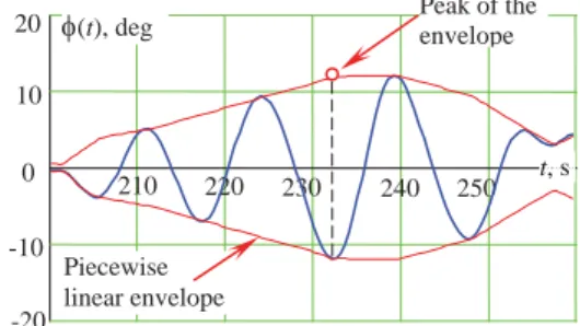
Ship motions are characterized by strong dependence of the data points on each other, especially in following and stern quartering seas when a spectrum is narrow and autocorrelation function takes a long time to decay. However, the peaks of the piecewise linear envelope (see Figure 1) represent independent data points. The difference between piecewise linear and theoretical
envelope is considered by Belenky and Campbell (2012). However, this technique may not work for the cases of parametric roll, where mutual dependence is much stronger. The method of collecting independent data for the case of parametric roll is described in Kim, et al.( 2014).
Figure 1: Piecewise linear envelope and its peak
3.2 Estimating Shape and Scale Parameters
To facilitate the choice of the threshold at a later step, fitting the shape and scale parameters are carried out for a series of prescribed thresholds. The maximum likelihood estimator (MLE) method is a standard way of estimating the parameters for the GPD. The idea of MLE method is quite intuitive: to find such values of parameters that are “most likely” to fit the data.
What is “most likely”? The data points that have been observed are the facts. At the same time they are instances of a random variable. Because these particular values were observed, they are more likely to occur than others. That means that the probability of observing these particular values reaches maximum when the correct parameters are used for distribution. The parameters are found by maximizing the value of the likelihood function. In practice this is made easier by taking the natural logarithm of the likelihood function (Equation 8 below).
210 220 230 240 250
-20 -10 0 10 20
t, s
I(t), deg
Piecewise linear envelope
P ¸ ¹ · ¨ © § V [ ¸¸ ¹ · ¨¨ © § [ V V [
¦
i i n i i x z z n l 1 1 ln 1 1 ) ln( ) , ( (8)Where n is the number of data points above a threshold P, zi are the sample data points above
a threshold P(sometimes referred to as
excesses).
3.3 Distribution the GPD Parameters
Since the shape and scale parameters are estimated from the envelope peak data (which are random numbers), the estimated parameters are also random numbers. Their distribution can be approximated with a bivariate normal distribution (Smith, 1987).
¸ ¸ ¹ · ¸ ¸ ¹ · V [ U ¨ ¨ © § V [ ¨ ¨ © § U U S V [ V [ V [ [V V V [ [ [V [V V [ V V E E V E V E V V fN ) ˆ )( ˆ ( 2 ) ˆ ( ) ˆ ( ) 1 ( 2 1 exp 1 2 1 ) ˆ , ˆ ( 2 2 2 2 (9)
Here [ˆ and Vˆ are estimates of ȟ and ı,Eis used for expected (or mean) value, V is the variance and U is the correlation coefficient between ȟ and ı. The parameter estimates produced by maximizing equation (8) are the mean values, while the covariance matrix MC is
found using the method outlined below.
¸ ¸ ¹ · ¨ ¨ © § U U V V [ [V V [ [V [ V V V V V V
MC (10)
The delta method allows one to find the estimates of mean and variance of the output, if estimates of the input are known and the function that turns input into output can be linearized, such as by a Taylor series. Because of this the delta method is an approximation.
Appling the delta method to maximization of equation (8) yields the Fisher information matrix MF that is an inverse of the covariance
matrix (10) (Boos and Stefanski, 2013):
¸ ¸ ¸ ¸ ¹ · ¨ ¨ ¨ ¨ © § V w V [ w [V w [ w V [ w [V w [ w V [ w [ w V [ w 2 2 2 2 2 2 ) , ( ) , ( ) , ( ) , ( l l l l
MF (11)
The derivatives in (11) are expressed as follows:
¦
¦
¦
[ V ¸¸ ¹ · ¨¨ © § [ [ V [ ¸ ¹ · ¨ © § V [ [ [ w V [ w n i i i n i i i n i i z z z z z l 1 2 2 1 2 1 3 2 2 1 1 2 1 ln 2 ) , ( (12)¦
V[ ¸¸ ¹ · ¨¨ © § [ V [ V w V [ w n
i zi
n l 1 2 2 2 2 1 1 1 ) , ( (13)
¦
¦
[ V ¸¸ ¹ · ¨¨ © § [ [ V [ V [ V w [ w V [ w n i i i n i i z z z n l 1 2 1 2 2 2 1 1 1 1 ) , ( (14)The covariance matrix is finally found as:
1
F
C M
M (15)
Figure 2: Joint distribution of GDP parameters
It is important to note that the scale parameter is by definition a positive quantity, while the bivariate normal distribution formally supports negative values for the scale parameter. To avoid negativity of V as an artifact of approximation (9), Pipiras, et al. (2015) proposed using the lˆV lnVˆ instead of
V This leads to a new distribution:
¸ ¸ ¹ · ¸ ¸ ¹ ·
[ U
¨ ¨ ©
§
[ ¨
¨ © §
U
U S
[
V [
V V [ V [
V V V
[ [
V [
V [ V [ V
l l l
l l
l
l l
LN
V V
E l E
V E l V
E V V l
f
) ˆ )( ˆ ( 2
) ˆ ( ) ˆ (
) 1 ( 2
1 exp
1 2
1 )
ˆ , ˆ (
2 2
2
2
(16)
V [V V [ V V V V V
U U
E E
V V E
El ln ; l 2; l (17)
Difference between distribution (16) and bivariate normal (9) is not very large (Pipiras,
et al., 2015).
3.4 Choice of the Threshold
Choosing a correct threshold is a critical to ensuring the applicability of the GPD. If the threshold is too low, the fitted GPD is not an approximation of the tail, because the conditions of the second extreme value
theorem have not been met. If the threshold is too high, “eligible” data have been wasted and the result will more scatter or uncertainty than necessary.
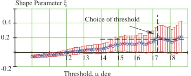
The second extreme value theorem states that the GPD can be used for approximation of the tail of any distribution if the threshold is high enough. That means that above certain threshold the GPD approximation must be invariant to the threshold (Coles, 2001). The simplest way is to observe stabilization of the shape parameter, see Figure 3.
Figure 3 Choice of threshold by stabilization of the shape parameter
Campbell, et al. (2014) describes study of five different methods of setting the threshold:
1. Stabilization of shape parameter
2. Stabilization of modified scale parameter 3. Stabilization of mean residual life estimate 4. Ad-hoc method based on minimum absolute difference between the shape parameter and its median above the threshold
5. Ad-hoc method based on minimum squared difference in the shape from its mean above the threshold
The first three methods are taken from Coles (2001) and they were mostly intended for “manual” calculation with “a human in a loop”. The methods 4 and 5 are similar to the methods proposed in Reiss and Thomas (2007) for automatic choice of the threshold. The referred study (Campbell, et al., 2014) has shown that automation of the method 1 through 3 makes the threshold lower than the visual choice. For the example shown in Figure 3, these methods put the threshold somewhere V
fN([V
[
12 13 14 15 16 17 18 -0.2
0.2 0.4
Shape Parameter [
Threshold, P deg
around 13~14 degrees, while the visual choice is somewhere above 17 degrees.
At the same time methods 4 and 5 have returned the threshold that is more close to the “visual” choice. The method 4 is quickly reviewed below. It is based on minimizing the following function:
¦
[ [ [P
1
) ˆ ,.., ˆ ( ian d e m ˆ ) (
1 1 )
(
Tr
Tr
N
k i
N k i
b Tr
Tr k
i N
k N
f
(18)
The value of b was taken as 0.5; NTr is the
number of the thresholds considered. A plot of (16) is shown in Figure 4. A global minimum (ignoring that the function goes to zero at the right) occurs just below P=17.4 deg, which is close to one of the visual choices made at Figure 3.
Figure 4 Choice of the Threshold based on the Global Minimum of the Equation (16)
4. EXTRAPOLATION AND UNCERTAINTY OF THE
PROBABILITY OF EXCEEDANCE
4.1 Extrapolated Estimate
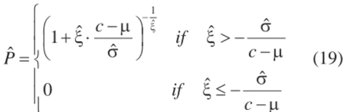
Using the GPD to extrapolate the probability of exceedance yields the conditional probability that the level of interest
c has been exceeded if the threshold P has been exceeded:
° ° ¯ ° ° ®
P V d [
P V ! [ ¸
¹ · ¨
© §
V P [
[
c if
c if
c
P
ˆ ˆ
0
ˆ ˆ
ˆ ˆ 1 ˆ
ˆ 1
(19)
c is the limit that constitutes the stability failure. The probability that ȝ has been exceeded can be estimated statistically, since it has been exceeded often enough so that we have enough data to build the distribution of peaks above it.
Now let’s consider the problem of the right bound. As can be seen from equation (19), the probability of exceedance is equal zero for negative shape parameters and ctPVˆ/[ˆ . This has several implications.
First, the extrapolated estimate is a random number. The joint distribution of the shape and scale parameters is approximated using distribution (16). That also means that the mean values of the shape and scale parameters are the most probable values at the same time (because normal distribution has a maximum at its mean value). Thus, one could expect that the most probable values used for formulae (19) returns the most probable value of extrapolated estimate.
So if the formula (19) returns zero, it is the most probable answer, but not the only one possible. In fact, the formula (19) must be accompanied with confidence interval that may be seen as a “range of answers”.
4.2 Mean and Distribution of the Extrapolated Estimate
In contrast to the most probable value of the extrapolated estimate, the mean value is never zero for a finite volume of data. Consider formula (19) as a deterministic function of random arguments:
V [ˆ,ˆ ˆ g
P (20)
10 12 14 16 18 20 0
0.1 0.2 0.3
Its mean value can be found as using well known formula for the mean value of deterministic function of random arguments:
³ ³
f f f V [ V [ V [ 0 ) , ( ) , ( ) ˆ(P g f d d
E LN (21)
Using (21) the PDF of the extrapolated estimate is derived as:
P [[ ¸ ¹ · ¨ © § P [ [ [ [ f f [
³
d c x x x c f xfp LN
2 1 2 1 1 , ) ( (22)
Figure 5 depicts the PDF of the extrapolated estimate
Figure 5: PDF of the Extrapolate Estimate (Campbell, et al., 2014).
More details are available from Campbell et al. (2014). The formula (22) also can be written using the bivariate normal distribution (9).
4.3 Confidence Interval of the Extrapolated Estimate
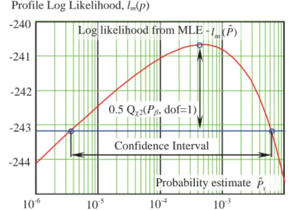
Quantiles of distribution (22) can be used to evaluate the confidence interval of the extrapolated estimate. The profile log likelihood PLL method (Coles, 2001) adapted for the extrapolated estimate is another way to find the confidence interval (Campbell, et al., 2014). The log likelihood estimator (8) is expressed in terms of the extrapolated estimate
Pˆ (19):
¦
[ [ ¸ ¸ ¹ · ¨ ¨ © § ¸¸ ¹ · ¨¨ © § [ ¸ ¸ ¹ · ¨ ¨ © § [ [ n i i p c P z P c n P l 1 1 ˆ 1 ln ˆ 1 1 1 ˆ ˆ ln ) ˆ , ˆ ( (23)and maximized by the shape parameter:
) ˆ , ˆ ( max arg ) ˆ (
ˆ p x
x
m P l P
l [
[
(24)
and the extrapolated estimate:
) ˆ ( max arg ˆ
ˆ m x
P P l P x (25)
The difference between them, referred as deviance statistic D and is assumed to have Ȥ2 distribution: ) ˆ ( ) ˆ ( ) ˆ
(Px lm P lm Px
D (26)
The confidence interval includes the space where: ) 1 , ( 5 . 0 )
(p QF2 PE dof
D (27)
Pȕ is the confidence probability and QȤ2 is the
quantile function of the Ȥ2 distribution. The boundaries are found as the limits of Px that
satisfy the condition (27), see Figure 6.
Figure 6. Profile Log Likelihood Method for Confidence Interval (Campbell, et al. 2014)
Pipiras, et al. (2015) systematically studied and compared different methods of calculating the confidence interval for the extrapolated
10-3 -244 -243 -242 -241 -240
Profile Log Likelihood, lm(p)
10-4
10-5
10-6
Confidence Interval 0.5 QF2(PE, dof=1) Log likelihood from MLE -lm(Pˆ)
Probability estimate Pˆx
estimate. The following methods were considered:
1. Delta method
2. "Normal" method ( distribution 9) 3. "Lognormal" method (distribution 22) 4. "Boundary" method
5. Standard bootstrap method
6. Profile likelihood method (as briefly described above)
In addition to those six methods, three more techniques, termed indirect techniques, investigated were based on quantiles rather than extrapolated estimate for exceedance probability. Any of the methods mentioned above can be used to construct a confidence interval for the return level (the level to be exceeded with given probability p):
1[
V [
p
xp (28)
The general scheme of calculations of the confidence interval through quantiles / return level is shown in Figure 7. The three methods adapted to the indirect approach using quantiles were:
7. Indirect "Lognormal" method 8. Indirect "Boundary" method 9. Indirect Profile likelihood method
Figure 7 On Calculation of Confidence Interval using quantiles (Pipiras, et al., 2015)
A comparison study was performed on simulated data sampled from a GPD distribution. The performance was judged based on the percentage of cases where the confidence interval contained the true value
(coverage). An accurate method should have the coverage close to the given confidence probability (PE=0.95). There were two series of calculations with 100 and 50 samples each.
The indirect profile likelihood method was shown to have the best performance, see Pipiras, et al. (2015). The delta method does not perform well for probability estimates and should not be used. The "normal", "log-normal", and indirect “log-normal” methods are slightly anticonservative (coverage < 95%) with the log-normal method preferred among the tree. The boundary method and indirect boundary methods are slightly conservative (coverage > 95%). The bootstrap and profile likelihood methods performed poorly for negative and near-zero shape parameters.
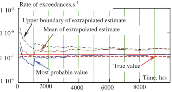
4.4 Convergence Study
Campbell, et al. (2014) describes convergence study for the EPOT method, using of the datasets from Smith et al. (2014) and Smith and Zuzick (2015). The results are shown in Figure 8.
The convergence test uses a moving average for 100 extrapolation data sets; the moving average is performed for the most probable value, mean value, and the upper boundary of the confidence interval calculated with the “log-normal” method. The most probable value is a better estimator when the sample volume is large, while the mean shows better (and more conservative) performance for smaller sample volumes. More details are available from Campbell, et al., (2014).
Figure 8 Convergence Test Using Moving
0 2000 4000 6000 8000 1 10-5
1 10-6
1 10-7
1 10-8
Rate of exceedances,s-1
Upper boundary of extrapolated estimate Mean of extrapolated estimate
Most probable value
True value Time, hrs
Pˆ
LOW
Pˆ PˆUP
c xp
-ln(P) p
xˆ
p
x lowˆ
p
Averages to Approximate Extrapolated Estimates (Campbell, et al., 2014)
4.5 On the Validation of EPOT
A comprehensive validation study of the EPOT method is reported by Smith and Zuzick (2015). Motions of the ONR Tumblehome topsides (Bishop et al., 2005) configuration were simulated with a 3-DOF volume-based simulation (Weems and Wundrow, 2013; Weems and Belenky, 2015) for hundreds of thousands of hours to produce “true” values on rare exceedances. Than small subsets (100 hrs each) was used by EPOT extrapolation. Smith and Zuzick (2015) used log-normal and boundary methods in carrying out their validation procedure for six relative wave headings considering roll, pitch, lateral and vertical accelerations. Using the same data set, Pipiras,et al. (2015) reported results for heave and pitch only for 30 and 45 degrees of heading, but used methods 2 through 9 for the confidence interval.
Total number of conditions reported by Smith and Zuzick (2015) was 23. The minimal acceptable coverage was set to 90%. With log-normal confidence interval six conditions failed, while all the conditions are passed using the boundary method. These results could be expected as the log-normal method is slightly anti-conservative and the boundary method is slightly conservative, as mentioned above. Smith and Zuzick (2015) noted that all the conditions show acceptable results for restricted range of headings – aft of the beam seas. Similar conclusions were reached by Pipiras,et al. (2015).
5. CURRENT STATUS AND FUTURE WORK
The EPOT method has evolved significantly in the three years since the previous STAB conference. The main idea remains the same, however: extrapolate peaks
over a threshold and use the envelope to ensure independence. The idea of threshold was originally aimed to emphasize influence of nonlinearity. Now it is also has a mathematical interpretation – it ensures the applicability of the second extreme value theorem.
Use of the second extreme value theorem leads to use of the Generalized Pareto distribution (GPD) to approximate the distribution above a certain large threshold. The selection of the threshold is done based on applicability of GPD approximation above the chosen threshold. Five different techniques for selecting the threshold have been considered.
Fitting the GPD is performed with the maximum likelihood estimation (MLE) method. These parameter estimates from the MLE fit are assumed to follow a normal distribution. Several methods were considered for estimating the confidence interval of the extrapolated probability of exceedance. Some of them we anti-conservative and some were conservative. A definitive recommendation on which to use is still outstanding.
Significant progress has been achieved in the validation techniques of EPOT and the problems of extreme rarity in general. A very fast simulation code has been developed that is capable of producing statistics for events that occur only a few times during millions of hours. The simulation was shown to be qualitatively similar to higher fidelity codes like LAMP (Weems and Belenky, 2015). A procedure for the validation of statistical extrapolation techniques has been developed and applied to EPOT (Smith and Zuzick, 2015). While not all the tested environmental conditions satisfied the currently proposed requirements, the EPOT method shows promise and potential to be acceptable.
relationship between the GPD parameters and physical considerations can be established. Pipiras, et al. (2015) investigated fixing the ratio between the GPD parameters for the case of pitch based on shape of the longitudinal GZ curve. This resulted in decreasing of width of the confidence interval and spread of the estimates around the “true” value. Such a decrease of uncertainty was the result of introducing additional physical information into the problem. The idea of a limiting roll angle is discussed by Campbell, et al (2015) and may lead to a similar result for roll. It is anticipated that further study into the nature of the tail of the distribution of large ship motions will lead to an application-ready EPOT method.
6. ACKNOWLEDGEMENTS
The work described in this paper has been funded by the Office of Naval Research, under Dr. Patrick Purtell, Dr. Ki-Han Kim and Dr. Thomas Fu. The authors greatly appreciate their support. The participation of Prof. Pipiras was facilitated by the Summer Faculty Program supported by ONR and NSWCCD under Dr. Jack Price (David Taylor Model Basin, NSWCCD). The authors would like to acknowledge fruitful discussions with Prof. Pol Spanos (Rice University), Dr. Art Reed, Mr. Tim Smith (David Taylor Model Basin, NSWCCD), and Prof. Ross Leadbetter (University of North Carolina ,Chapel Hill).
7. REFERENCES
Belenky, V. and Campbell, B.L., 2012 “Statistical Extrapolation for Direct Stability Assessment”, Proc. 11th Intl. Conf. on Stability of Ships and Ocean Vehicles STAB 2012, 243-256, Athens, Greece.
Belenky, V., Weems, K. and Lin, W.M., 2015 “Split-time Method for Estimation of Probability of Capsizing Caused by Pure Loss of Stability” in Proc. 12th Intl. Conf. on Stability of Ships and Ocean Vehicles
STAB 2015, Glasgow, UK.
Bishop, R. C., W. Belknap, C. Turner, B. Simon, and Kim J. H., 2005 “Parametric Investigation on the Influence of GM, Roll damping, and Above-Water Form on the Roll Response of Model 5613.” Report NSWCCD-50-TR-2005/027.
Boos, D. D. and Stefanski, L. D., 2013 Essential Statistical Inference: Theory and Method. Springer.
Campbell, B. and Belenky, V., 2010 “Assessment of Short-Term Risk with Monte-Carlo Method” Proc. 11th Int. Ship Stability Workshop, Wageningen, the Netherlands.
Campbell, B., Belenky, V. and Pipiras, V., 2014 “Properties of the Tail of Envelope Peaks and their Use for the Prediction of the Probability of Exceedance for Ship Motions in Irregular Waves” CSM7 Computational Stochastic Mechanics, Deodatis, G. and P. D. Spanos, eds. (accepted).
Campbell, B., Belenky, V. and Pipiras V., 2014a “On the Application of the Generalized Pareto Distribution for Statistical Extrapolation in the Assessment of Dynamic Stability in Irregular Waves” Proc. 14th Intl. Ship Stability Workshop, Kuala Lumpur, Malaysia, pp. 144-148.
Coles, S., 2001 An Introduction to Statistical Modeling of Extreme Values. Springer, London.
David, H. A. and Nagaraja, H. N., 2003. Order Statistics. Wiley Series in Probability and Statistics
Kim, D.H., Belenky, V., Campbell, B. L. and Troesch, A. W., 2014 “Statistical Estimation of Extreme Roll in Head Seas” in Proc. of 33rd Intl. Conf. on Ocean, Offshore and Arctic Engineering OMAE 2014, San-Francisco, USA.
Kobylinski, L. and Kastner, S. 2003 Stability and Safety of Ships. Regulation and Operation, Elsevier.
McTaggart, K. A., 2000 “Ongoing Work Examining Capsize Risk of Intact Frigates Using Time Domain Simulation”. In Contemporary Ideas of Ship Stability, D. Vassalos, et al. (eds), Elsevier Science, pp. 587–595.
McTaggart, K. A., de Kat J.O., 2000 “Capsize Risk of Intact Frigates in Irregular Seas”. Trans. SNAME, Vol. 108, pp 147–177.
Pickands, J., 1975 “Statistical Inference Using Extreme Order Statistics”. The Annals of Statistics Vol. 3, No 1, pp. 119-131.
Pipiras, V., Glotzer, D., Belenky, V., Campbell, B., Smith, T., 2015 "Confidence Interval for
Exceedance Probabilities with Application to Extreme Ship Motions", J. of Statistical Planning and Inference (Submitted)
Reed, A., Beck, R. and Belknap, W., 2014 “Advances in Predictive Capability of Ship Dynamics in Waves”, Invited Lecture at 30th Symposium of Naval Hydrodynamics, Hobart, Australia.
Reiss, R.-D. and Thomas, M., 2007 Statistical Analysis of Extreme Values with Application to Insurance, Finance, Hydrology and Other Fields. 3rd Edition, Basel: Birkhäuser Verlag.
Smith, R. L., 1987 “Estimating tails of probability distributions.” The Annals of Statistics Vol 15, pp.1174–1207.
Smith, T. C., 2014 “Example of Validation of
Statistical Extrapolation Example of Validation of Statistical Extrapolation,” Proc. of the 14th Intl. Ship Stability Workshop, Kuala Lumpur, Malaysia.
Smith, T. C., and Zuzick, A., 2015 “Validation of Statistical Extrapolation Methods for Large Motion Prediction” in Proc. 12th Intl. Conf. on Stability of Ships and Ocean Vehicles (STAB 2015), Glasgow, UK.
Weems, K., and Wundrow, D., 2013 “Hybrid Models for Fast Time-Domain Simulation of Stability Failures in Irregular Waves with Volume-Based Calculations for Froude-Krylov and Hydrostatic Forces”, Proc. 13th Intl. Ship Stability Workshop, Brest, France.