Hemodynamic Response Function Modeling
Wenjie Chen
A dissertation submitted to the faculty of the University of North Carolina at Chapel Hill in partial fulfillment of the requirements for the degree of Doctor of Philosophy in the Department of Statistics and Operations Research (Statistics).
Chapel Hill 2012
Approved by:
Young K. Truong
Haipeng Shen
J. S. Marron
Aysenil Belger
c
2012
Wenjie Chen
Abstract
WENJIE CHEN: Hemodynamic Response Function Modeling. (Under the direction of Young K. Truong and Haipeng Shen.)
Functional Magnetic Resonance Imaging (fMRI) is a medical-imaging technique for studying brain function. It can be used to capture the response of the brain to various tasks. The response to a brief, intense period of neural stimulation is called the hemodynamic response function(HRF). Modeling HRF is essential to identifying the brain activation by exploring the relationship between the experimental stimulus and the response.
In this dissertation, we discuss three research problems related to HRF estima-tion. First, when multiple types of stimuli are present, how can we capture the char-acteristic HRF for each stimulus? Second, is there any difference among the HRFs corresponding to multiple stimuli? Third, how can we improve the HRF estimator’s efficiency?
We propose a nonparametric method,transfer function estimate(TFE), to answer these three questions. Building on existing work, we extend the nonparametric ap-proach to a multivariate form, which adapts to the multiple types of stimuli, and we develop hypothesis testing to identify the brain activation and to compare the HRFs under different stimuli. In order to improve estimation efficiency, we propose using
Acknowledgments
I would like to pay tribute to my advisors, Drs. Shen and Truong, for their enthusiasm, vision, and immense knowledge. I treasure their guidance in the past five years of my Ph.D. study and research.
I would like to thank as well my other committee members: Dr. Belger, Dr. Bhamidi, and Dr. Marron for their support and helpful comments.
Dr. Huang created an invaluable research environment. Her encouragement, passion, and advice motivated me to better myself and my work.
I wish to thank Mechelle and Suman for the consistent support they gave me during the years. Their kindness, patience, and help in the lab bolstered my research and warmed my heart.
I thank Dr. Belger and Joshua for the chance to work with them, and for the scientific and psychiatric interpretations they provided.
My memory of fMRI is with Seonjoo. And the computation platform would have been a hard bump without Gu.
Contents
Abstract . . . iii
List of Figures . . . viii
List of Abbreviations . . . x
1 Introduction . . . 1
1.1 Functional Magnetic Resonance Imaging . . . 1
1.2 Experimental Design . . . 3
1.3 Hemodynamic Response Function and Its Application . . . 5
1.3.1 HRF . . . 5
1.3.2 Application . . . 7
1.4 Overview . . . 9
2 Literature Review . . . 10
2.1 A Model for BOLD Signals . . . 10
2.2 HRF Modeling . . . 12
2.2.1 Time Domain Methods . . . 13
2.2.2 Frequency Domain Methods . . . 15
2.2.3 Comparison of the Current Methods . . . 16
2.2.4 Nonparametric HRF Modeling . . . 17
3 Methodology: Three New Developments in HRF Modeling . . . . 22
3.1 Multivariate Form of HRF Modeling: Transfer Function Estimate . . 22
3.1.1 Window Estimate . . . 26
3.1.2 Multiple Smoothing Parameters . . . 28
3.1.3 Coherence . . . 29
3.1.4 Partial Coherence . . . 29
3.2 Hypothesis Testing . . . 30
3.3 Weighted Least Square . . . 35
3.4 Introduction of Modified Cross Validation . . . 37
4 Simulation Study. . . 39
4.1 Simulation 1: Various Experimental Designs . . . 39
4.1.1 Event-Related Design . . . 41
4.1.2 Block Design . . . 42
4.2 Simulation 2: Multiple Stimuli . . . 43
4.3 Simulation 3: Modified Cross Validation . . . 45
4.4 Simulation 4: Hypothesis Testing . . . 46
4.5 Simulation 5: Weighted Least Squares . . . 48
4.6 Simulation 6: Face Data Design . . . 51
4.7 Advantages of TFE . . . 53
5 Real Data Application . . . 72
5.1 Detecting Activation in Auditory Data . . . 72
5.2 HRF Modeling in Finger-Tapping Data . . . 75
5.2.1 TR Issues . . . 77
5.2.2 Brain Map . . . 82
5.4 Event-Related Visual Data . . . 85
6 Sampling Properties . . . 92
6.1 Sampling Properties of Multiple HRFs Estimation . . . 92
6.1.1 Bias of Hˆ(r) . . . 96
6.1.2 Covariance of Hˆ(r) . . . 103
6.1.3 Normality ofHˆ(r) . . . 105
6.1.4 Normality ofhˆ(·) . . . 107
6.2 Properties of Hypothesis Testing Procedure . . . 109
6.3 Sampling Properties of Weighted Least Square . . . 111
6.3.1 Best Linear Unbiased Estimator (BLUE) . . . 113
6.3.2 Convergence in Probability . . . 116
7 Conclusion . . . 118
List of Figures
1.1 Two major types of experimental designs . . . 4
1.2 A typical HRF . . . 6
4.1 HRF modeling with three different experimental designs . . . 40
4.2 Multivariate HRF estimation from the regular block design . . . 56
4.3 The HRF estimation result of TFE by using different (longer or shorter than the true value) input length . . . 57
4.4 The MCV simulation study on random event-related design . . . 58
4.5 The multivariate HRF estimation from the regular block design by using MCV . . . 59
4.6 The simulated brain map in Simulation 4 . . . 60
4.7 Detecting the activation regions with identical HRFs . . . 61
4.8 Hypothesis testing with two identical HRFs in the simulated brain . . 62
4.9 Detecting the activation regions by TFE with non-identical HRFs . . 63
4.10 Hypothesis testing with two non-identical HRFs in the simulated brain. 64 4.11 The experimental design for the five-method comparison . . . 65
4.12 HRF estimates from typical block design . . . 66
4.13 HRF estimates from the simulation that only show response to one of the stimuli in block design. . . 67
4.14 Face data design . . . 68
4.15 TFE estimates in 200 face data simulations . . . 69
4.16 AFNI and sFIR estimates in the face data simulation . . . 70
5.2 F map and T map of the activation by using TFE and SPM . . . 74
5.3 Finger-tapping design . . . 76
5.4 Detrended time series from one voxel in finger-tapping data . . . 77
5.5 TFE in the left primary motor cortex (PMC) . . . 78
5.6 TFE in the left supplementary motor area (SMA) . . . 79
5.7 TFE in right cerebellum area . . . 80
5.8 The HRF estimates in the activated region of left PMC . . . 81
5.9 Activation maps of right hand task . . . 83
5.10 The activation map generated by TFE in the face data . . . 84
5.11 The activation map generated by SPM in the face data . . . 85
5.12 HRF estimates in one voxel from face data . . . 86
5.13 Event-related visual data design . . . 87
5.14 The activation detected by SPM in event-related visual data . . . 88
5.15 The activation detected by TFE in event-related visual data . . . 89
List of Abbreviations
AFNI Analysis of Functional NeroImages
BOLD Blood Oxygenation Level Dependent
FIR Finite Impulse Response
fMRI functional Magnetic Resonance Imaging
FSL FMRIB Software Library
GLM General Linear Model
HRF Hemodynamic Response Function
ITI Inter-trial Interval
MCMC Markov chain Monte Carlo
MCV Modified Cross Validation
MR Magnetic Resonance
OLS Ordinary Least Square
RMSE Root Mean Squared Error
ROI Region of Interest
SPM Statistical Parametric Mapping
SVD Singular Value Decomposition
TFE Transfer Function Estimate
Chapter 1
Introduction
A brief background of functional Magnetic Resonance Imaging (fMRI) and the modeling of hemodynamic response function(HRF) will be described along with our research projects. Section 1.1 introduces a powerful tool, fMRI, widely used in neu-romedical imaging studies. Two categories are suggested in Section 1.2 for classifying the experimental designs in terms of stimulus presentation. Section 1.3 describes HRF in fMRI and its application under two types of experimental designs. Section 1.4 gives motivation and discusses the contribution of our research in HRF modeling.
1.1
Functional Magnetic Resonance Imaging
While studying the human brain 200 years ago, phrenologists introduced the idea oflocalization of function: the brain may have distinct regions that support particular mental processes, that is, different aspects of the human mind may be represented in different brain regions (Huettel, Song, and McCarthy, 2004). This localization idea inspires modern-day explorers to map the human brain by localizing different mental processes to different parts of the brain; one popular analysis tool is fMRI, which is used to take images of the active brain in both clinical and research settings.
moreover, it can also reveal short-term physiological changes associated with the active functions of the brain. FMRI is a leading technique in creating the maps of human brain function by using standard magnetic resonance (MR) scanners.
Functional MRI is a measure of metabolic activity, instead of neural activity. It is well established that energy metabolism and neural activity are tightly coupled. The activity of neuron requires energy from the metabolism which is provided sufficiently by blood flow in the brain. A small neuronal activity could cause a large increase in local energy demand. The energy comes from the consumption of glucose and oxy-gen in the blood. The oxyoxy-gen is attached to hemoglobin molecules. The oxygenated hemoglobin (Hb) and deoxygenated hemoglobin (dHb) have different magnetic prop-erties in MR scanner. There are more MR signal when Hb is at a high level and less MR signal when dHb is at a high level. The changes of the dHb level can be captured in a strong static magnetic field from MR scanner.
FMRI is able to measure the signal of the delivery of oxygen and glucose to active neurons. Theblood-oxygen-level dependent (BOLD) signal from the MR scanner has been shown to be closely linked to neural activity. Through a process called the
hemodynamic response, blood releases oxygen to active neurons at a greater rate than to inactive ones. Most fMRI studies measure changes in blood oxygenation over time. Because blood oxygen levels change rapidly following the activity of neurons in a brain region, fMRI allows researchers to localize brain activity on a second-by-second basis and within millimeters of its origin. The brain activity is mapped onto a structural brain image highlighting the activation regions, called brain mapping. The spatial resolution of the cubic-millimeter-volume units (the basic three-dimension sampling units are known asvoxels) forms the brain mapping; the temporal resolution of seconds improves the precision of the hemodynamic response study.
is, with respect to a volume unit voxel, data in the form of time series are analyzed in a proper model to obtain the brain mapping. The time series data, which we will denote later as{Y(t);t= 0, . . . , T−1}, come from one voxel; as the brain is composed of millions of voxels, for the whole brain, millions of time series can be detected in the MR scanner during the experiment. The experimental stimuli{s(t);t= 0, . . . , T−1}
will be designed in a particular way for the MR scanner to detect the corresponding changes in the brain. When the stimulus is present,s(t) is 1; otherwise, it is 0.
A typical neuropsychological test in fMRI is the finger-tapping experiment: the participant is signaled to perform finger tapping in the MR scanner according to the experimental paradigm {s(0), . . . , s(T −1)}, and at each voxel, the fMRI data Y(t) is recorded during both finger-tapping {t :s(t) = 1} and rest {t :s(t) = 0} periods. The signal received by the subject is the stimulus. In one voxel from the brain, we can start the analysis from the two series: the fMRI dataY(t) and its known stimulus function s(t). The relationship between Y(t) and s(t) is used for detecting whether the voxel is responsive to the stimulus or not.
The experimenters are interested in detecting the brain regions activated by the stimulus, as well as understanding the mechanism by which the brain responds to the stimulus.
1.2
Experimental Design
In this section, we discuss the stimulus functions(t) from two typical experimental designs for fMRI.
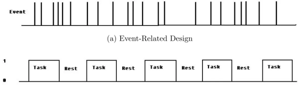
of one event-related design, where the locations of the peaks correspond to the event times. A block design separates experimental conditions into distinct blocks, and each experimental condition is presented for an extended period of time. For example, see Figure 1.1b, where each block corresponds to the duration of the experiment stimulus.
(a) Event-Related Design
(b) Block Design
Figure 1.1: Two major types of experimental designs. (a) illustrates a random event-related design. Each vertical line over time represents one event (a single stimulus). (b) illustrates a block design. Each block represents a period of stimulus presentation. There is a certain amount of resting periods between them.
For a simple example, there is only one kind of stimulus in the experiment. Figure 1.1a and 1.1b can be regarded as an illustration of the time series of the stimulus function {s(t) :t= 1, . . . , T}, where s(t) equals 1 for stimulus presentation and 0 for resting.
Thus, the relationship between the multiple stimulus functions and the fMRI response is much more complicated than in the simple one-stimulus design.
1.3
Hemodynamic Response Function and Its
Ap-plication
The change in the MR signal triggered by neural activity is known as the hemo-dynamic response. The relationship between the stimulus s(t) and the BOLD signal
Y(t) involves hemodynamic response function (HRF). Estimating or determining the HRF is important for the correct interpretation of neurological studies.
The HRF is the response to a brief, intense period of neural stimulation. The shape of the HRF varies according to the properties of the stimulus and, presumably, the underlying neuronal activity. The components of the typical HRF include a peak and a post-dip (undershoot) as shown in Figure 1.2. The peak is the maximum amplitude of the HRF, occurring typically about 4 to 6 seconds following a short-duration event. The undershoot is the decrease in MR signal amplitude below baseline due to the combination of reduced blood flow and increased blood volume.
Hemodynamic response varies from region to region in the brain and from subject to subject during the same experiment. Increasing the rate of neural firing increases HRF amplitude, whereas increasing the duration of neural activity increases HRF width (latency).
1.3.1
HRF
Figure 1.2: This is a typical HRF as double gamma functions, called Glover’s HRF (Glover, 1999). It is composed by the peak and the post-dip indicated in the plot. Itsx-axis refers to time, and itsy-axis refers to the intensity of HRF. Usually a HRF lasts 20 to 30 seconds.
peak and undershoot.
Initial Dip
At the first 1 to 2 seconds after stimulus, an initial dip is reported by many studies. While neuronal activities start in a neuron region, the transient energy demand is satisfied by the oxygen extraction in local Hb. This results an increase of dHb, and therefore the decrease of MR signal, called initial dip.
Peak
Undershoot
After the peak, the blood flow decreased more rapidly than the blood volume to the baseline. During the period that the blood flow returns to baseline and the blood volume is still above the baseline, a greater amount of dHb is present, and therefore the MR signal is below the baseline for a prolonged period, called undershoot.
The typical shape of HRF contains an initial dip, a rise to peak, a fall to baseline, and a prolonged post-stimulus undershoot. As the initial dip lasts only 1 to 2 seconds, it may not be detected without finer temporal resolution of MR signal. Different persons may have different HRF shapes including the timings of rise and fall, the amplitude of the peak, and the HRF latency. However, the connection from neuronal activity to energy metabolism is about the same. BOLD signal is regarded as a detector of the neural activity and the functions of the brain.
1.3.2
Application
A single stimulus can evoke a hemodynamic response in the brain that spans a 20-second or greater latency. For each trial, the duration of the BOLD response matches well with the subject’s response time (Richter, Ugurbil, Georgopoulos, and Kim, 1997). The shape and intensity of the hemodynamic response varies across brain regions and across individuals. Thus, when investigating the activity using fMRI, we must consider its spatial and temporal properties.
The HRF typically is closely linked to the event-related stimulus in fMRI, be-cause the design paradigm allows the HRF to return to baseline or to recover after every trial. By characterizing the precise timing and waveform of the hemodynamic response, researchers can make inferences about the relative timing of neuronal ac-tivity, neuronal feedback processes, and sustained activity within a brain region.
been demonstrated that the areas of BOLD activity can be detected using even very short-duration stimuli and interstimulus intervals. In event-related designs, stimuli that generate short bursts of neural activity are known as events or trials. The dif-ferent conditions are usually presented in random order rather than an alternating pattern. Event-related studies measure transient changes in brain activity associated with discrete stimuli. The pattern of changes over time becomes critical for exper-imental analysis. The characteristics of the event-related designs make the precise estimation of the timing and the waveform of a given HRF achievable. On the other hand, block designs are good for detecting brain activation regions, but are not widely used in estimating the HRF. Most existing HRF estimators have been developed un-der event-related design. We propose a procedure for estimating the HRF that works under both event-related and block designs.
A basic assumption for estimating HRF is linearity. In the event-related design, we consider the hemodynamic response to be evoked by a single, isolated stimulus; in the block design, the stimuli are presented in succession, and it is possible to assume that the same HRF is evoked for every stimulus, independently of the other stimuli presented. If the stimuli are sufficiently close together so that their hemodynamic responses overlap, then the measured total change in MRI signal will be the sum of the individual processes, known as a linear system (Boynton, Engel, Glover, and Heeger, 1996; Friston, Worsley, Frackowiak, Mazziotta, and Evans, 1993).
1.4
Overview
Estimating HRF is our initial inspiration for improving fMRI analysis. In the process of building up the theorems and the methodology for HRF, we developed several ways to generate function maps. As the final goal of fMRI study is to give human brain mapping, the methodology we present in this dissertation is an analyzing system about dealing with fMRI data based on HRF estimation.
In our work, we investigate frequency domain approaches for estimating the HRF in fMRI. We first extend the approach of Bai, Huang, and Truong (2009) from event-related designs to block designs. Then we improve estimation efficiency. For the application purpose, we also develop an estimation approach that can incorporate multiple stimuli in one experimental design. A hypothesis-testing procedure is devel-oped to identify the voxels activated by a certain stimulus and to compare the effects from different stimuli. In the following chapters, we illustrate the performance of our estimators and the testing procedure using simulation studies and real fMRI applica-tions. Finally, we prove the sampling properties of the HRF estimation: consistency and efficiency.
Chapter 2
Literature Review
In this chapter, we review a few popular methods for fMRI data analysis and the HRF modeling.
2.1
A Model for BOLD Signals
In an experiment design with a single type of stimulus, the BOLD response Y(t) acquired from the scanner is supposed to fluctuate with the stimulus activated at times τ1 < τ2 <· · ·. A popular model for the BOLD response (Friston et al., 1993)
is the linear time invariant system:
Y(t) = X
u
h(t−τu) +(t), (2.1.1)
whereh(·) is the HRF and(t), t= 0,1, . . . , T−1 is a stationary, 0-mean noise series. Typically, a hemodynamic response lasts for 20 to 30 seconds, that is, h(u) = 0 when
u <0 andu > d for some positive constant d. Model (2.1.1) can also be written as
Y(t) =
d
X
u=1
h(t−u)s(t) +(t), t = 0, . . . , T −1, (2.1.2)
convolution model, where the BOLD response is modeled as the convolution of HRF and the stimulus function s(·). When there are n stimuli, then model (2.1.2) can be extended to
Y(t) =
d
X
u=1
h1(t−u)s1(t) +· · ·+
d
X
u=1
hn(t−u)sn(t) +(t), t= 0, . . . , T−1. (2.1.3)
The General Linear Model Framework
As one of the most popular approaches, the general linear model (GLM) models the BOLD signal as a linear combination of several different component predictors. It is used to test whether the activity in a brain region is systematically related to any of those known input functions (Lindquist, 2008). The data input for fMRI analysis includes the responseY(t) of the voxel at timet, and also the stimulus function s(t). Considering the relationship between the stimulus and the response, the GLM was first elucidated by Friston, Holmes, Worsley, Poline, Frith, Frackowiak, et al. (1995b). It may be expressed as
Y =Xβ+ (2.1.4)
The parameter vector β will be estimated in each voxel to weigh the effect of each experimental predictor.
As the HRF h(·) is involved as part of the predictor from the design matrix X, an accurate hemodynamic response can improve the statistical power of the fMRI modeling analysis. Under the GLM framework, many studies looked into the design matrix X and tried to capture the characteristics of the hemodynamic response, and to come up with valid predictors. Mumford and Nichols (2006) summarized the GLM framework and its implementation in various fMRI softwares. Some studies (Zhang, Lu, Johnstone, Oakes, and Davidson, 2008; Casanova, Ryali, Serences, Yang, Kraft, Laurienti, and Maldjian, 2008) also explore the error correlation structure to improve the efficiency of the estimation. Lindquist, Meng Loh, Atlas, and Wager (2009) furthermore propose some consequent statistical inference after estimating HRF.
When multiple stimuli are presented in succession, the hemodynamic response is often assumed to be the summation of the individual responses generated by the each stimulus respectively (Dale and Buckner, 1997). Under certain conditions, the fMRI response has been found to be approximately linear (Hykin, Bowtell, Glover, Coxon, Blumhardt, and Mansfield, 1995; Boynton et al., 1996), and this has been the basis for most of the event-related fMRI analysis to date (Buckner, Bandettini, OCraven, Savoy, Petersen, Raichle, and Rosen, 1996; Cohen, 1997; Friston, Fletcher, Josephs, Holmes, Rugg, and Turner, 1998a). GLM adapts to multiple-stimulus through the cooperation of multiple columns in the design matrix X based on the linearity as-sumption.
2.2
HRF Modeling
is easily obtained from the convolution model (2.1.2). Most studies in the GLM framework obtain predictors based on known HRFs, and plug them into the design matrix X, so as to test whether the predictors are able to detect the activities. A variety of fixed HRFs has been used in early studies, such as the Poisson function (Friston, Jezzard, and Turner, 1994), the Gamma function (Cohen, 1997; Lange and Zeger, 1997; Friston, Josephs, Rees, and Turner, 1998b) and the Gaussian function (Rajapakse, Kruggel, Maisog, and Von Cramon, 1998; Kruggel and von Cramon, 1999; Dale and Buckner, 1997). After Glover (1999) intensively investigated the shape of the HRF, the typical HRF shape (Figure 1.2) is suggested in the form of a double Gamma function. Since then the double Gamma function has been widely used in fMRI studies and popular fMRI data analysis packages, such as Statistical Parametric Mapping (SPM), FMRIB Software Library (FSL), and Analysis of Functional NeuroImages (AFNI). For example, the double Gamma function is the canonical HRF in SPM, which is the default choice.
Because the HRF varies across individuals and across brain regions, there exists no fixed “standard” form of HRF. It is crucial to allow flexibility in the exact HRF form while analyzing fMRI data; otherwise, even minor mismodeling of the HRF can result in severe power loss, and can inflate the false positive rate beyond the nominal level.
There is a list of literature on estimating HRF using fMRI data. Below we have or-ganized the literature into two major categories: time domain and frequency domain, which will be reviewed in sections 2.2.1 and 2.2.2.
2.2.1
Time Domain Methods
form of a product of a sine function and exponential functions, which model the early and late components of an evoked hemodynamic response. Bullmore, Bram-mer, Williams, Rabe-Hesketh, Janot, David, Mellers, Howard, and Sham (1996) and Zarahn (2000) choose the sinusoidal orthogonal basis functions. Josephs, Turner, and Friston (1997) use two sine basis functions. Lindquist and Wager (2007) model the HRF using a superposition of three inverse logit functions. Jacobs, Hawco, Kobayashi, Boor, LeVan, Stephani, Siniatchkin, and Gotman (2008) and Steffener, Tabert, and Stern (2009) employ Fourier basis sets to model the HRF. In general, the more basis functions are used in a linear model, the more flexible the model is in estimating the parameters of the GLM. However, flexibility relies on the cost of more free parame-ters, which means more error in estimating HRF, fewer degrees of freedom, and less statistical power due to potential collinearity.
Several Bayesian methods have also been developed in HRF modeling. Genovese (2000) uses the polynomial “bell” function to indicate the rise, fall, decay, and dip parts of the HRF. G¨ossl, Fahrmeir, and Auer (2001) derive the method based on physiological assumptions with the posterior estimated by numerical or Markov chain Monte Carlo (MCMC) methods. In Friston, Penny, Phillips, Kiebel, Hinton, and Ashburner (2002), an empirical Bayesian approach is taken to model the HRF with basis functions under constraints. Woolrich, Jenkinson, Brady, and Smith (2004) present a fully Bayesian approach using the addition of four half-period cosines with six constrained parameters to account for the variation of HRF. All these Bayesian approaches require imposing restrictions on the HRF parameters.
time-domain deconvolution method still has the collinearity problem, especially for the periodic experimental designs. Lu, Bagshaw, Grova, Kobayashi, Dubeau, and Gotman (2006; 2007) compare the performance between three fixed HRFs (Gamma HRF, Glover HRF, and SPM canonical HRF) and the deconvolution method under the framework of GLM. Goutte, Nielsen, and Hansen (2000) propose a semiparametric approach based onfinite impulse response (FIR) filters, which have more flexibility in modeling HRF. Zhang, Jiang, and Yu (2007; 2008) propose a semiparametric method that uses smoothing splines to estimate the drift function and the HRF while care-fully taking into account the covariance structure within the BOLD signal. However, the semiparametric methods of Goutte et al. (2000) and Zhang et al. (2007; 2008) require some specific assumption of the covariance structure, which might not be correct. And both methods are computationally expensive. More recently Lindquist et al. (2009) compare several HRF estimating methods based on simulation and real data analysis, including SPM (Statistical Parametric Mapping) canonical HRF with or without its temporal or dispersion derivatives, FIR, semiparametric FIR, and the inverse logit model. So far, we can see that the “standard” HRF estimation lacks the natural spatial variability of HRF, and the model-driven approach generally has collinearity problems.
2.2.2
Frequency Domain Methods
domain to simplify convolution evaluations and for easier accommodation of tempo-ral and spatial autocorrelation. Marchini and Ripley (2000) offer a frequency domain method for the periodic stimuli with self-calibrating. It detects activation on the fundamental (stimulus-related) frequency and harmonics of the stimulus design per voxel with the information from other frequencies to calibrate its statistic. For HRF modeling, Makni, Beckmann, Smith, and Woolrich (2008) propose a nonparametric HRF estimate using fully Bayesian inference through Markov Chain Monte Carlo (MCMC) at the price of a high computational demand. Another frequency-domain method is Wink, Hoogduin, and Roerdink (2008) based on the Fourier-wavelet regu-larized deconvolution technique. Bai et al. (2009) implement a nonparametric model for estimating the HRF using fast Fourier transformation of event-related fMRI data. We describe the technical details in the next chapter, as our work builds upon their method.
2.2.3
Comparison of the Current Methods
Most existing analytical techniques for fMRI data need specific assumptions about the HRF. These assumptions may not be appropriate when the HRF varies from subject to subject or from region to region, especially for the pre-specified HRF methods. Sometimes the experiment contains more than one type of stimulus, and the application for the parametric methods may not be adapted for the multiple stimuli. Additionally, it is unlikely that the fMRI data is homogeneous from the whole scanning session, so the error correlation structure should be considered in the analysis, the estimation of which could be another difficulty in fMRI modeling.
Zeger (1997) and Marchini and Ripley (2000) both outline the frequency approaches depending on the pre-defined HRF. They lack the ability to specify the HRF variation or adapt to the different types of stimulus design (Figure 1b, 1c). Bai et al. (2009) implement a nonparametric model of estimating HRF in the event-related experimen-tal design. Their method exploits the experimenexperimen-tal designs by modeling the stimulus sequences using a stochastic point process and accounts for the variability of HRFs across regions of brain. The method is proposed only in a single event-related design, and we extend this method to block design and the design that allows the multiple, overlapping events throughout an experiment, such as rapid event-related design. We describes their method in the following section for future reference.
2.2.4
Nonparametric HRF Modeling
In order to understand our method better in terms of terminology, such as the derivation of its name, we first define the system transfer function by
H(r) = X
υ
h(υ) exp(−iυr), r∈R (2.2.1) where r is the radian frequency. Practically, we use the finite Fourier transform
ϕY(r)≡ϕτY(r) = T−1
X
t=0
exp(−irt)Y(t) (2.2.2)
with a similar definition for ϕX(r) and ϕ(r), r∈R. It follows from (2.1.2) that
ϕY(r) = H(r)ϕX(r) +ϕ(r), r∈R. (2.2.3)
By fast Fourier transform,ϕY(·) andϕX(·) are obtained on the Fourier frequencies
Bai et al. (2009) exploits the experimental designs by modeling the stimulus se-quences using point process and accounts for the variability of HRFs across regions of brain. Here we describe some details given in Bai et al. (2009) to help understand our methodology. Note that this method is in a univariate form.
Let mr denote the integerm ∈ {0, . . . , T −1} such that 2πmr/T is closest to the
angular frequency r∈(0, π/2). Then for the smooth H(·),
ϕY(
2π
T (mr+k))≈H(r)ϕX(
2π
T (mr+k)) +ϕ(
2π
T (mr+k)) (2.2.4)
for allk = 0,±1, . . . ,±K, whereK is a positive integer. As we can see,{2π
T (mr+k)}k
are the nearest 2K+ 1 frequencies aroundramong the Fourier frequencies. Equation (2.2.4) is a linear regression system which can offer a reasonable estimate of H(r), denoted by ˆH(r).
ˆ
H(r) = ˆfY X(r)/fˆXX(r) (2.2.5)
where
ˆ
fXX(r) = (2K+ 1)−1 K
X
k=−K
IXX(
2π
T (mr+k)), (2.2.6)
ˆ
fY X(r) = (2K+ 1)−1 K
X
k=−K
IY X(
2π
T (mr+k)), (2.2.7) IXX(r) = (2πT)−1ϕX(r)ϕX(r), (2.2.8)
IY X(r) = (2πT)−1ϕY(r)ϕX(r), (2.2.9)
where A is the conjugate of A. In practice, a smoother estimate known as the window estimate is used by observing that (2.2.6) and (2.2.7) can be written as
ˆ
sXX(r) =
X
k6=0
b−1W(b−1(r− 2πk
T ))IXX(
2πk
ˆ
sY X(r) =
X
k6=0
b−1W(b−1(r− 2πk
T ))IY X(
2πk
T ), (2.2.11)
where W(·) is a weight function called a (spectral) window, and b is the smoothing parameter. ˆsXX(r) is called power spectrums and ˆsY X(r) is cross-spectrum. It has
been shown that the window estimate has better sampling properties than (2.2.8) and (2.2.9) as an estimate of the cross-spectrum of the bivariate time series.
With the defined smoothed power spectrums, ˆsXX(·) and ˆsY Y(·), the stimulus
point processX(t) and the stationary time seriesY(t), and the estimate of the cross-spectrum ˆsY X(·), the estimation of H(·) is
ˆ
H(r) = ˆsY X(r)/sˆXX(r). (2.2.12)
Consequently the estimate of the impulse response functionh(·) is then given by the inverse Fourier transform.
For the statistical inference for detecting the activity, Bai et al. (2009) define the squared coherence as
|RˆXY(r)|2 =
|ˆsXY(r)|2
ˆ
sXX(r)ˆsY Y(r)
, r ∈R. (2.2.13)
Under certain conditions, ˆRXY(r) is asymptotically normal with a meanRXY(f) and
variance proportional to the constant (1−R2
XY(r))/T. Moreover, ifRXY(r) = 0, then
F(r) = c| ˆ
RXY(r)|2
1− |RˆXY(r)|2
∼ F2,2c, (2.2.14)
where c is a constant that depends on the smoothing parameters. The F statistic can then be used to test whether there is any response at the task-related frequency
2c degrees of freedom. An F(r) value, which is larger than the presumed threshold, indicates a significant effect at the task-related frequency.
2.3
Popular Softwares in FMRI
the times at which neurons fire. (To make a PSTH, a spike train recorded from a single neuron is aligned with the onset, or a fixed phase point, of an identical stimulus repeatedly presented to an animal. The aligned sequences are superimposed in time, and then used to construct a histogram.)
FSL (Woolrich, Jbabdi, Patenaude, Chappell, Makni, Behrens, Beckmann, Jenk-inson, and Smith, 2009; Smith, JenkJenk-inson, Woolrich, Beckmann, Behrens, Johansen-Berg, Bannister, De Luca, Drobnjak, Flitney, et al., 2004) also applies GLM to data. By default, FSL uses a single gamma function with temporal derivatives as HRF. It also has options on convolving with Gaussian function, double gamma function, and basis functions such as gamma, sine, and FIR. Furthermore, FSL has another approach to directly tune the HRF to make the optimal basis functions with four half-period cosine components. Also when the constraints for the HRF parameters are chosen, the basis function is automatically generated in FSL using singular value decomposition (SVD).
Chapter 3
Methodology: Three New Developments
in HRF Modeling
This chapter focuses on the methodology of our developments in HRF modeling. Section 3.1 presents our first development: transfer function estimate (TFE), an HRF estimating method which incorporates the multiple stimuli in fMRI study. Following the multiple stimuli discussion, the multivariate tests are introduced in Section 3.2. In Section 3.3, we propose an efficient HRF estimator. To estimate the smooth parameter included in the computing process, Section 3.4 discusses our proposal for the analysis of fMRI time series.
3.1
Multivariate Form of HRF Modeling: Transfer
Function Estimate
over successive trials is beneficial for experiment design.
The method used by Bai et al. (2009) reviewed in Chapter 2 is set up for the types of stimulus with the univariate HRF involved in the experiment design; however, different stimuli may evoke varying HRFs even in the same location of the brain. For instance, there are two types of stimulus, A and B, in one scanning session. Stimulus A may stir up a much higher (or lower) response than Stimulus B; in terms of HRF shapes, it means a larger (or smaller) amplitude. Also the brain may have a quicker reaction to Stimulus A; in terms of HRF shapes, it proposes a different timing estimation for the lag. In brief, it is possible for stimuli A and B to have totally different HRF shapes. Additionally, more than two types of stimuli can be applied in the scanning session, making the analysis even more complicated.
Note that linearity assumption also works in multiple stimuli sessions. BOLD signal is basically the summation of all the HRFs evoked by any kind of stimulus.
The multivariate form of HRF modeling, calledtransfer function estimate (TFE), provided the statistical inference between different types of stimuli.Its name comes from the definition of Equation (2.2.1). Not only does the multivariate form give sep-arate estimates of HRFs from different stimuli, but also the hypotheses on the same shape of HRFs among different stimuli are built on the multivariate model. Com-paring the shapes of HRF is also of high interest in fMRI research. The hypotheses support some assumptions in fMRI, such as varying responses to the multiple speci-fied stimuli. After the hypothesis testing, if it is acceptable to conclude that two kinds of stimuli have the same HRF shapes in the voxel of one subject, then the number of variates in the model decreases, which increases the statistical power for estimating HRF.
As the extension to the convolution model (2.1.2), the multivariate HRF model is
where xi(·) represents theith stimulus function and hi is the corresponding HRF.
Let X(t) be an n vector-valued series, that is, X(t) = (x1(t), x2(t), . . . , xn(t))τ.
Then suppose that h(u) is a 1×n filter as h(u) = (h1(u), h2(u), . . . , hn(u)). The
HRF model (3.1.1) we are concerned with have the form
Y(t) = X
u
h(u)X(t−u) +(t). (3.1.2)
We assume that the error series, (t), is stationary with 0 mean and power spectrum
s(r), and that the HRF h(u) is 0 when u < 0 or u > d, where d is the length of
HRF determined by underlying neural activity. We can calculate the finite Fourier transform
ϕX(r)≡ϕ
(T)
X (r) =
T−1
X
t=0
X(t) exp(−irt). (3.1.3)
LetK be an integer with 2πK/T near radian frequency r. SupposeT is large. From the asymptotic property of finite Fourier transform,
ϕY(
2π(K+k)
T ) ˙=H(r)ϕX(
2π(K +k)
T ) +ϕ(
2π(K+k)
T ), k = 0,±1, . . . ,±m.
Relation (3.1.4) is seen to have the form of a multiple regression involving complex-valued variates. In a matrix form, the linear system (3.1.4) is
ΦY(r) =
ϕY(2Tπ(K−m))
ϕY(2Tπ(K−m+ 1))
.. .
ϕY(2TπK)
.. .
ϕY(2Tπ(K +m))
,ΦX(r) =
ϕX(2Tπ(K−m))τ
ϕX(2Tπ(K−m+ 1))τ
.. .
ϕX(2TπK)τ
.. .
ϕX(2Tπ(K +m))τ
τ ,
Φ(r) =
ϕ(2Tπ(K−m))
ϕ(2Tπ(K−m+ 1))
.. .
ϕ(2TπK)
.. .
ϕ(2Tπ(K+m))
,
then we use ordinary least square (OLS) to estimate H(·),
ˆ
H(r) = (ΦX(r)ΦX(r)τ)−1ΦX(r)ΦY(r)τ. (3.1.5)
We call (3.1.5) uniform estimate of Hˆ(·) as later we will define window estimate. To make an easy extension in notation, alternatively we define
IYX(r) = (2πT)−1ϕY(r)ϕX(r)
τ
, (3.1.6)
IXX(r) = (2πT)−1ϕX(r)ϕX(r)
τ
, (3.1.7)
ˆfYX(r) = (2m+ 1)−1
m
X
k=−m
IYX(
2π(K+k)
ˆfXX(r) = (2m+ 1)−1
m
X
k=−m
IXX(
2π(K+k)
T ). (3.1.9)
Suppose that the n×n matrixˆfXX(r) is non-singular. We now write (3.1.5) as
ˆ
H(r) =ˆfYX(r)ˆfXX(r)−1 (3.1.10)
and estimatef(r) by
ˆ
f(r) =
2m+ 1
2m+ 1−r[ ˆfY Y(r)−ˆfYX(r)ˆfXX(r)
−1ˆf
XY(r)]. (3.1.11)
The transfer function H(r) is estimated by expression (3.1.10). And the estimate of
h(u) we consider
ˆ
h(u) = 1
T
T−1
X
t=0
ˆ H(2πt
T ) exp(i2πtu/T). (3.1.12)
Thus, ˆh is the final HRF estimate from TFE.
3.1.1
Window Estimate
observing (3.1.8) and (3.1.9), the window estimate can be written as
ˆsYX(r) =
m
X
k=−m
W(2πk
T )IYX(
2π
T (K+k))
=
K+m
X
k=K−m
W(2π(k−K)
T )IYX(
2πk T )
=
K+m
X
k=K−m
W(2πk
T −r)IYX(
2πk T )
=
K+m
X
k=K−m
W(r− 2πk
T )IYX(
2πk T )
where W(·) is a non-negative function called the weight or window function. Since the estimation process is required to be symmetric, we extend the weight function periodically.
W(α+ 2π) = W(α),
Note that IYX(0) = 0. In order to reflect the notion that the weight function should
become more concentrated as the sample sizeT tends to∞, we introduce a bandwidth parameter b that depends on T (Brillinger, 1981) such that b → 0 as T → ∞, then for sufficiently large T,
Z 2π
0
b−1W(b−1α)dα= 1. (3.1.13) We therefore consider the following general window estimates:
ˆsYX(r) =
X
k6=0
b−1W(b−1(r− 2πk
T ))IYX(
2πk
T ), (3.1.14)
ˆsXX(r) =
X
k6=0
b−1W(b−1(r− 2πk
T ))IXX(
2πk
T ), (3.1.15)
and estimateH(r) by
ˆ
Then we have
ˆ
h(u) = 1
T
T−1
X
t=0
ˆ H(2πt
T ) exp(i
2πtu
T ). (3.1.17)
3.1.2
Multiple Smoothing Parameters
We can write down (3.1.14) and (3.1.15) as
ˆsYX(r) =
X
k6=0
W((r− 2πk
T ), b)IYX(
2πk
T ), (3.1.18)
ˆsXX(r) =
X
k6=0
W((r− 2πk
T ), b)IXX(
2πk
T ), (3.1.19)
whereW(u, b) is ann×nweight matrix with{W(u, b)}ij =W(u, b), i, j ∈ {1, . . . , n}.
The n HRFs corresponding to the n types of stimuli may have different smooth-ness, which requires different smoothing parameters for each HRF estimation. The proposed way to perform the multiple smoothing is to specify differentbiin the weight
matrix W(s, b). We can simply extend (3.1.18) and (3.1.19) to useW(u, b), ann×n
weight matrix with {W(u, b)}ij =W(u, bi), i, j ∈ {1, . . . , r}. The matrix forms are
ˆsYX(r) =
P
k6=0b
−1 1 W(b
−1
1 (r− 2πkT ))IY x1(
2πk
T )
P
k6=0b
−1 2 W(b
−1
2 (r− 2πkT ))IY x2(
2πk
T )
.. .
P
k6=0b
−1
r W(b
−1
n (r− 2πkT ))IY x3(
2πk T ) τ , (3.1.20)
ˆsXX(r) =
P
k6=0b
−1 1 W(b
−1 1 (r−
2πk
T ))I
[1]
XX(
2πk
T )
P
k6=0b
−1 2 W(b
−1 2 (r−
2πk
T ))I
[2] XX( 2πk T ) .. . P
k6=0b
−1
r W(b−n1(r− 2πkT ))I
[r]
XX( 2πk T ) , (3.1.21)
and I[XXi] (·) denotes the ith row of the matrix IXX(·). The smoothing parameters for
HRFs (h1(·), h2(·), . . . , hn(·)) are (m1, m2, . . . , mn).
When the smoothing parameters are different, the ˆsXX(r) may not be
positive-definite. In practice, the task sequences of many experiments vary little, and so it seems reasonable to apply our procedure using the same smoothing parameters.
3.1.3
Coherence
Coherence is an important statistic that provides a measure of the strength of a linear time invariant relation between the series Y(t) and the series X(t); that is, it indicates whether there is a strongly linear relationship between the BOLD response and the stimulus. From a statistical view, we can test the linear time invariant assumption for the convolution model; for the fMRI exploration, we can choose the voxels with significantly large coherence where the BOLD series have functional responses to the stimulus, and then estimate the HRF in those voxels.
Coherence is defined as
|RYX(r)|
2
=sYX(r)sXX(r)−1sXY(r)/sY Y(r). (3.1.22)
Coherence is seen as a form of correlation coefficient, bounded by 0 and 1. The closer to 1, the stronger linear time invariant relation between Y(t) and X(t).
3.1.4
Partial Coherence
If we look at the stimuli individually, it is interesting to consider the complex analogues of the partial correlations, or partial coherence. The estimated partial cross-spectrum of Y(t) andXi(t) after removing the linear effects ofXj(t) is given by
sYXi·Xj(r) =sYXi(r)−sYXj(r)sXjXj(r)
−1
Usually, the point of interest is the relationship between the response and a single stimulus after other stimuli are accounted for; that is, Xi is the single stimulus of
interest, and Xj is the other stimuli involved in the design paradigm.
The partial coherence of Y(t) and Xi(t) after removing the linear effects of Xj(t)
is given by
RY Xi·Xj(r)
2
= sY Xi·Xj(r)
2
sY Y·Xj(r)sXiXi·Xj(r)
. (3.1.24)
Ifn = 2, that is, if there are two kinds of stimuli in the experiment, it can be written as
RY Xi·Xj(r)
2
=
RY Xi(r)−RY Xj(r)RXiXj(r)
2
[1−RY Xj(r)
2
][1−RXiXj(r)
2
]. (3.1.25) Partial coherence is especially important when we focus on a specific stimulus. Not all stimuli are considered in equal measure. Stimuli such as the heart beat and breathing, which cannot be avoided in any experiment involving humans, are of secondary concern. Furthermore, as each type of stimulus has its own characteristics, it is natural to perform an individual statistical analysis to see how each one affects the overall fMRI response.
3.2
Hypothesis Testing
Testing Linearity
fMRI hemodynamic response.
It is possible that the nonlinearity is overwhelmed during scanning. Consequently, it is crucial to make sure that the linearity assumption is acceptable. The advantage of our method is that we can first determine whether the linearity assumption is acceptable before using the convolution model for analysis.
The value of coherence, between 0 and 1, reflects the strength of the linear re-lation between fMRI response and the stimuli. Under certain conditions, ˆRYX(r)
is asymptotically normal with mean RYX(r) and variance proportional to constant
(1−R2YX(r))/T b. Moreover, ifRYX = 0, then
F(r) = (c−n)| ˆ
RYX(r)|2
n(1− |RˆYX(r)2|)
∼ F2n,2(c−n) (3.2.1)
where c = bT /γ and γ = R κ2 with κ being the lag-window generator depending on the choice of window function. If the F statistic on coherence is significant, it is reasonable to accept the linearity assumption.
Testing the Effect from a Specific Stimulus
For each brain area, stimuli have varying effects. For the motor cortex in the left hemisphere, right-hand motion causes much more neural activities than left-hand motion. Partial coherence is able to distinguish between right- and left-hand effects, determine whether left-hand motion evokes neural activity, and identify which motion has greater effect. The following test is applied for these kinds of research questions.
For partial coherence, if RY Xi·Xj = 0, then
F(r) = c
0|ˆ
RY Xi·Xj(r)|
2
1− |RˆY Xi·Xj(r)2|
∼ F2,2(c0−1) (3.2.2)
where c0 =bT /γ−n+ 1 andγ =R
Detecting the Activation
HRF in fMRI indicates the arising neural activity. If there is activation evoked by the stimulus, then the corresponding HRF cannot be ignored. If there is no HRF in a brain region, there is no going-on neuronal activity. To detect activation in the brain region is to see whether there is underlying HRF. For our frequency method, we test H(r0) = 0 at stimulus-related frequencyr0.
We are interested in testing the hypothesisH(r) = 0. This is carried out by means of analogs of the statistic (3.1.22). In the case of H(r) = 0,
(bT /γ)Hˆ(r)ˆsXX(r)Hˆ(r)τ
nˆs(r)
(3.2.3)
is distributed asymptotically as F2;2(bT /γ−n).
Testing the Difference between HRFs
The multiple-stimulus method simplifies the functional hypothesis testing by com-paring the corresponding Fourier coefficients at frequency r in order to see whether there is any discrepancy between HRF curves corresponding to different stimuli. HRFs curves are functions, but when we focus just on Fourier coefficients at fre-quency r, we look at a common hypothesis testing on points. To see the difference between the two HRFs, it is enough to consider the hypothesis that the two Fourier coefficients at task-related frequency r0 are equivalent.
As we know, H(·) is the Fourier transform of the form
H(r) =
T−1
X
t=0
h(t) exp(−irt) (3.2.4)
with the h(·) real-valued. For the contrast hypothesis to compare HRF functions
is usually the task-related frequency r0.
In OLS method, we know the distribution of Hˆ(r)τ is asymptotically
NrC(H(r)τ, s(r)Σ) H(λ)∈Cn (3.2.5)
where Σ=
(bT /γ)−1ˆs
XX(r)−1 r6= 0 modπ
(bT /γ−1)−1ˆs
XX(r)−1 r= 0 modπ
NrC(·,·) is the complex multivariate normal distribution for the r vector-valued ran-dom variable.
Definition 3.2.1. The Complex Multivariate Normal Distribution. IfΣ=Σ1+ iΣ2
is a complex-valued m×m matrix such that Σ=Στ and aτΣa ≥0 for all a∈
Cm,
then we say that Y = Y1 + iY2 is a complex-valued multivariate normal random
vector with meanµ=µ1+ iµ2 and covariance matrix Σ if
Y1 Y2 ∼N
µ1 µ2 , 1 2
Σ1 −Σ2
Σ2 Σ1
. (3.2.6)
We then write Y ∼NmC(µ,Σ).
By the definition of complex normal distribution, then we have
Re Hˆ(r)τ
Im Hˆ(r)τ
∼N
Re H(r)τ
Im H(r)τ
,
1 2s(r)
Re Σ −Im Σ
Im Σ Re Σ
. (3.2.7)
Simply notate the multivariate normal as
ˆ
Hτv ∼N(Hv,
1
where Hv is in a 2n-dimensional real vector space,Hv =
Re H(r)τ Im H(r)τ
and Σv is a
2n×2n real matrix, Σv =
Re Σ −ImΣ
Im Σ ReΣ
.
The contrast between different HRF estimates can be represented by cτHˆ(r)τ,
where c= (c1, c2, . . . , cn)τ which satisfies that
Pn
i=1ci = 0. For the complex number
cτHˆ(r)τ, the hypothesis testing can be conducted by the definition of complex normal
distribution, which converts complex normal to multivariate normal distribution.
Under the hypothesis cτH(r) = 0, (c c)
Re Hˆ(r)τ Im Hˆ(r)τ
, denoted byc
τ
vHˆv, where
cτ
v = (c1, . . . , cn, c1, . . . , cn), is distributed asymptotically as
N
0,1
2s(r)c
τ vΣvcv
. (3.2.9)
At the same time the distribution of ˆs(r) is approximated by an independent
s(r)χ22(bT /γ−n)
2(bT /γ−n) r6= 0 modπ. (3.2.10) Thus, the t statistic for the contrast between different HRF estimates is
cτvHˆv(r)τ
q
2(bT /γ−n)
bT /γ ˆs(r)cτvΣ−v1cv
∼ t2(bT /γ−n) (3.2.11)
when r6= 0 mod π.
Left. Then we need to set up the contrast of conditions according to our interest. For testing whether the right hand has greater effect than the left hand, the contrast should be Right>Left, equivalent to Right−Left> 0. So we state the contrast in a vectorc= (1,−1), 1 for condition Right and−1 for condition Left. After settling the contrast, SPM and FSL will continue their general linear model, using parameters to conduct the t statistic.
The hypothesis of comparing the HRF similarity here equates the contrasts in SPM and FSL. We have two types of stimuli: Right and Left. Then we have respective HRF estimates for Right and Left. To test whether Right>Left, we specify c= (1,−1)τ in
cτHˆ(r)τ. As the result, t statistic in (3.2.11) is used for testing their difference.
3.3
Weighted Least Square
As shown in (3.1.5), we applied OLS to obtain the estimate ofH(·). The estimate (3.1.10) will be near an optimal estimate if s(r) is uniform. This is perhaps not
likely in fMRI data, since the BOLD response is not homogeneous throughout the whole experiment. The efficient estimate is given by WLS (its proof can be found in Chapter 6), where we used, in practice and in theory, the estimate ˆs(r) obtained by
the use of the same formulas given in (3.1.11) as the weight in the uniform estimate
ˆ
f(r) =
2m+ 1
2m+ 1−r[ ˆfY Y(r)−
ˆfYX(r)ˆfXX(r)−1ˆf
XY(r)].
The WLS estimate of the linear system (3.1.4) is
ˆ
where
Σ(r) =
ˆ
f−1(2Tπ(K−m)) ˆ
f−1(2Tπ(K−m+ 1)) . ..
ˆ
f−1
(
2π
T K)
. ..
ˆ
f−1
(
2π
T (K+m))
.
Then (3.1.8) and (3.1.9) are updated as
ˆf
YX(r) = (2m+ 1)−1
m
X
k=−m
ˆ
f−1(2π(K+k)
T )IYX(
2π(K+k)
T ), (3.3.2)
ˆfXX(r) = (2m+ 1)−1
m
X
k=−m
ˆ
f−1(2π(K+k)
T )IXX(
2π(K+k)
T ). (3.3.3)
For the general window estimate, the weight in WLS is
ˆ
s(r) =
bT /γ
bT /γ−r[ˆsY Y(r)−ˆsYX(r)ˆsXX(r)
−1ˆs
XY(r)]. (3.3.4)
Then the weighted spectrum is defined as
˜sYX(r) =
X
k6=0
b−1W(b−1(r− 2πk
T ))ˆs
−1
(
2πk T )ˆsYX(
2πk
T ), (3.3.5)
˜sXX(r) =
X
k6=0
b−1W(b−1(r− 2πk
T ))ˆs
−1
(
2πk T )ˆsXX(
2πk
The transfer function estimate is generally given by
˜
H(r) =˜sYX(r)˜sXX(r)−1 (3.3.7)
3.4
Introduction of Modified Cross Validation
We now describe one procedure for choosing the bandwidth (that is the window size) needed in our HRF estimation method. We refer to it asmodified cross validation
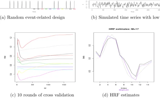
(MCV). MCV is basically a technique for assessing how well the results of statistical analysis in a time series can be generalized to an independent time series. For fMRI data, we use MCV for selecting the bandwidth in the spectrum smoothing during the procedure of TFE. For us, MCV is designed for HRF modeling to select the proper smoothing parameter M during the estimating procedure. The algorithm of MCV partitions a time series into consecutive subintervals, performing the analysis on one subinterval (called the training set), and validating the analysis on the other subinterval (called the testing set). To reduce variability, multiple rounds of MCV are performed by using different partitions, and the validation results are averaged over the rounds.
(that is, the number of testing subintervals), andwis the length of the testing interval. If a time series has length n, the algorithm of MCV is as follows.
1. Use the first n−qw time points as a training interval to estimate HRF, q =
Q, Q−1, . . . ,1.
2. Predict the nextwtime points by convolving the estimate HRF with the known stimulus sequence.
3. Calculate the Root Mean Squared Error (RMSE) on the predicted w time points.
4. Sum up the RMSE over the Q sequences, and select the smoothing parameter
M that minimizes the total RMSE.
The above procedure depends on the choice of Q and w. By default, we use
Q= 10 andw= 0.05n, which means 10 rounds of cross validation in the later half of the time series.
When two data sets—one set from theoretical prediction and the other from the actual measurement of some physical variable—are compared, the RMSE of the pair-wise differences in the two data sets can serve as a measure of how far on average the error is from 0. (The RMSE in the algorithm is to measure the expected level of fit of the model and here to determine the appropriate use of the smoothing parameter
Chapter 4
Simulation Study
We have several simulation studies corresponding to the three developments on HRF modeling. Section 4.1 applies the nonparametric method under rapid event-related design and block design. Section 4.2 is the simulation study of HRF estimate under a multiple-stimulus experiment. Section 4.3 validates the bandwidth selection method MCV in the simulation study. Then the multivariate hypothesis is tested in Section 4.4. The third development of estimation efficiency is verified in Section 4.5 through the comparison of WLS and OLS. Section 4.6 gives a comparison study on the specific experiment design called face data design among five current HRF modeling methods. By the end of the simulation study, we discuss the advantages of our method in Section 4.7.
4.1
Simulation 1: Various Experimental Designs
enough for the HRF to return completely to the baseline during non-stimulation. In common sense, the block design is not powerful at estimating the shape of the hemodynamic response (aside from its magnitude). However, TFE is powerful enough to be applied to all types of experimental designs.
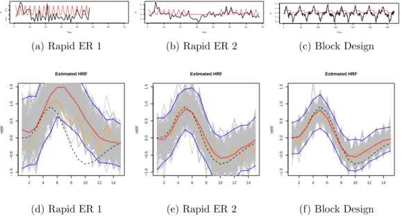
The simulation here follows the convolution model (2.1.2), where h is the Glover HRF (Glover, 1999), and (t) is white noise; that is, ∼ N(0, .25). The various experimental designs that follow are denoted by x(·).
Time
fz
0 10 20 30 40 50 60 70
−0.5
0.5
(a) Rapid ER 1
Time
fz
0 10 20 30 40 50 60 70
−1
0
1
2
(b) Rapid ER 2
Time
fz
0 50 100 150 200 250 300
−4
−2
0
2
4
(c) Block Design
2 4 6 8 10 12 14
−1.0 −0.5 0.0 0.5 1.0 1.5 HRF Estimated HRF
(d) Rapid ER 1
2 4 6 8 10 12 14
−1.0 −0.5 0.0 0.5 1.0 1.5 HRF Estimated HRF
(e) Rapid ER 2
2 4 6 8 10 12 14
−1.0 −0.5 0.0 0.5 1.0 1.5 HRF Estimated HRF
(f) Block Design
4.1.1
Event-Related Design
In Bai et al. (2009), the authors have shown that the method is successful in the single event-related design. Here we applied their method to the rapid event-related design.
The first simulation was the rapid ER-fMRI with a fixed ITI of 2 seconds (Figure 4.1a). We applied the method to the simulated data, obtaining 200 HRF estimates from the 200 simulations we ran. The results are shown in Figure 4.1d. The applica-tion of the method to the simulated rapid event-related design data resulted in HRF estimates that captured the original shape of HRF, represented by the dark red line in Figure 4.1d. The average of the estimates captured the shape of the true HRF, but it is above the true HRF dash line. The bias of the estimates comes from the experi-mental design: the stimulus frequency is so high that it keeps the HRF from reaching maximal values without returning to its baseline. Thus the estimates have a much higher peak than the true one without the post-dip. The results from this simulation led us to consider how to optimize the method and data to better estimate the HRF in rapid ER-fMRI. The second simulation gave us more information on experimental design parameters and improved estimation of the HRF.
by the thin original line) was now approximately superimposed on the average HRF and the experimental design. In this data analysis, the bias was largely removed and the estimate of the HRF shifted down to the correct position.
The improved results from the second simulation showed that the rest period was a crucial component of the experimental design. Even in the case when the stimulus frequency was high, we demonstrated that as long as there was one relatively long rest, we could still obtain good estimates of the hemodynamic response using our method. In summary, the advantages of this second experimental design include improved HRF estimates in rapid ER-fMRI.
4.1.2
Block Design
Even though block design is relatively insensitive to the HRF’s exact shape, in this section we apply our method under block experimental design to get the exact estimation of HRF. The simulation was set up with runs consisting of 16 blocks, with each block having a duration of 20 seconds. The block alternated between the stimuli and rest (Figure 4.1c). Based on the fact that the common hemodynamic response usually lasts around 15 seconds (as in the Glover HRF), we chose a block period of 20 seconds so that each block would not have any carry-over effect from the previous block. We then applied the method to this simulated data, obtaining 200 HRF estimates from the 200 simulations we ran. The results are shown in Figure 4.1f. The application of the method from Bai et al. (2009) to the simulated block design data resulted in HRF estimates that captured the original shape of HRF, represented by the dark red line in Figure 4.1c, with the 95% confidence interval designated by the blue lines above and below the red line. These data demonstrate that our adjusted method can extract the hemodynamic response pattern not only from event-related data (as in Bai et al. (2009)), but also from block design data. According to the estimates of the average HRF, however, we could see the relatively small bias in the estimates (the true HRF is the dashed line). The true HRF, however, is covered by the upper and lower bounds of the estimates.
4.2
Simulation 2: Multiple Stimuli
situations, we did the simulation in each situation.
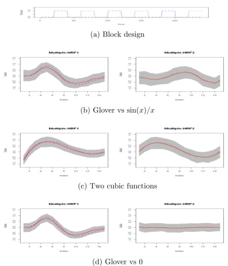
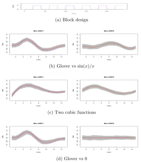
The simulations were built on the block design with two types of block interchang-ing (Figure 4.2a). There were enough rest periods for HRF so it would not affect the successive blocks. The first simulation was to estimate two different shapes of HRF, using Glover’s HRF and function
sin(2πx)
2x x=−2,−1.9,−1.8, . . . ,−.6. (4.2.1)
In Figure 4.2b, the dashed lines are the true HRFs, and the solid lines are the mean of estimates from 200 simulations with 95% gray band. As we can see, there is a large gap between the timing for peaks of Glover and sin(x)/x HRFs. Furthermore, the amplitudes of the two HRFs are not the same. As a result of dissimilar HRFs, the estimates from multivariate method fit the original HRFs well, separating the peaks and the amplitude from each other.
The second simulation (Figure 4.2c) had two similar HRFs functions: two cubic functions. The difference between the two cubic functions was subtle, from which we could only see a little difference in the starting point and undershoot period. Even though the difference was slight, the estimates still clearly identified the small difference between the two HRFs.
The third simulation (Figure 4.2d) states the possibility that there is no response to a stimulus. In Figure 4.2d, the second HRF is 0, which means no response exists for the second stimulus. The HRF estimates are consistent with the original ones, which confirms the confidence of using a multivariate method to estimate multiple HRFs.
to the input length. TFE has the advantage that it does not assume the length of HRF a priori, so the length of HRF does not affect the estimation performance of TFE, as shown empirically in Figure 4.3. In addition, the estimation results can give some suggestion about the support of the HRF. Furthermore, its result could give an estimate of the length of HRF. Figure 4.3 shows that the wrong HRF length could not affect the conducting result in TFE.
4.3
Simulation 3: Modified Cross Validation
As discussed in Section 3.4, MCV is used to choose bandwidth during the HRF estimating process. In Section 4.2, the smoothing parameter is chosen by hand or observation, which may not be efficient when dealing with noisy data or large data sets, since it is time consuming. In order to quickly choose a proper bandwidth in TFE, we introduced MCV and propose to use it in TFE.
In the simulations, we first set a standard way to select the smoothing parameter
M, which directly minimizes RMSE between the true HRF used in the simulation and the estimated HRF conducted by TFE.
We denoteh as a vector of true HRF (vector length isd) and ˆh(M) as a vector of the estimated HRF using smoothing parameter M
RM SE(M) = 1
d(ˆh(M)−h)
T(ˆh(M)−h).
For a single simulation, define Mopt as
In order to evaluate M obtained by MCV, we compare the HRF estimates gener-ated byMopt andM from MCV. The comparison on the random event-related design
with low Signal-to-Noise Ratio (SNR) is shown in Figure 4.4. The HRF estimates by using MCV is sustaining.
In addition, we illustrate the performance of the MCV procedure on the three simulation studies performed in Section 4.2. The true HRFs have different combina-tions. As we can see from Figure 4.5, the window sizes chosen by MCV give very nice HRF estimates, and in all three cases, they are close to the results corresponding to the subjectively chosen bandwidths in Figure 4.2.
4.4
Simulation 4: Hypothesis Testing
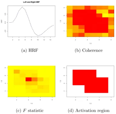
The simulation study was based on a multiple stimuli experiment design and a simulated brain. The experiment in the section included two types of stimuli, called left and right. The simulated brain had 8×8 voxels, which was designed to have various brain functions in the left and right experiment design. The brain was divided into four regions: One only responded to left, one only responded to right, one can respond to both left and right, and the remaining one had no response in the experiment.
The fMRI data was simulated based on the convolution model (3.1.1): the con-volution of the pre-specified left HRF h1(·) and right HRF h2(·), and the known
experiment paradigm for left stimulus x1(t) and right stimulus x2(t). The response
was given by