econ
stor
Make Your Publications Visible.
A Service of
zbw
Leibniz-Informationszentrum WirtschaftLeibniz Information Centre for Economics
Hemelt, Steven W.; Rosen, Rachel B.
Working Paper
School Entry, Compulsory Schooling, and Human
Capital Accumulation: Evidence from Michigan
IZA Discussion Papers, No. 9889
Provided in Cooperation with: IZA – Institute of Labor Economics
Suggested Citation: Hemelt, Steven W.; Rosen, Rachel B. (2016) : School Entry, Compulsory Schooling, and Human Capital Accumulation: Evidence from Michigan, IZA Discussion Papers, No. 9889, Institute for the Study of Labor (IZA), Bonn
This Version is available at: http://hdl.handle.net/10419/141648
Standard-Nutzungsbedingungen:
Die Dokumente auf EconStor dürfen zu eigenen wissenschaftlichen Zwecken und zum Privatgebrauch gespeichert und kopiert werden. Sie dürfen die Dokumente nicht für öffentliche oder kommerzielle Zwecke vervielfältigen, öffentlich ausstellen, öffentlich zugänglich machen, vertreiben oder anderweitig nutzen.
Sofern die Verfasser die Dokumente unter Open-Content-Lizenzen (insbesondere CC-Lizenzen) zur Verfügung gestellt haben sollten, gelten abweichend von diesen Nutzungsbedingungen die in der dort genannten Lizenz gewährten Nutzungsrechte.
Terms of use:
Documents in EconStor may be saved and copied for your personal and scholarly purposes.
You are not to copy documents for public or commercial purposes, to exhibit the documents publicly, to make them publicly available on the internet, or to distribute or otherwise use the documents in public.
If the documents have been made available under an Open Content Licence (especially Creative Commons Licences), you may exercise further usage rights as specified in the indicated licence.
Forschungsinstitut zur Zukunft der Arbeit Institute for the Study of Labor
DISCUSSION PAPER SERIES
School Entry, Compulsory Schooling, and Human
Capital Accumulation: Evidence from Michigan
IZA DP No. 9889
April 2016
School Entry, Compulsory Schooling,
and Human Capital Accumulation:
Evidence from Michigan
Steven W. Hemelt
University of North Carolina at Chapel Hilland IZA
Rachel B. Rosen
MDRCDiscussion Paper No. 9889
April 2016
IZA
P.O. Box 7240 53072 Bonn
Germany
Phone: +49-228-3894-0 Fax: +49-228-3894-180
E-mail: [email protected]
Any opinions expressed here are those of the author(s) and not those of IZA. Research published in this series may include views on policy, but the institute itself takes no institutional policy positions. The IZA research network is committed to the IZA Guiding Principles of Research Integrity.
The Institute for the Study of Labor (IZA) in Bonn is a local and virtual international research center and a place of communication between science, politics and business. IZA is an independent nonprofit organization supported by Deutsche Post Foundation. The center is associated with the University of Bonn and offers a stimulating research environment through its international network, workshops and conferences, data service, project support, research visits and doctoral program. IZA engages in (i) original and internationally competitive research in all fields of labor economics, (ii) development of policy concepts, and (iii) dissemination of research results and concepts to the interested public.
IZA Discussion Paper No. 9889 April 2016
ABSTRACT
School Entry, Compulsory Schooling, and Human Capital
Accumulation: Evidence from Michigan
*Extant research on school entry and compulsory schooling laws finds that these policies increase the high school graduation rate of relatively younger students, but weaken their academic performance in early grades. In this paper, we explore the evolution of postsecondary impacts of the interaction of school entry and compulsory schooling laws in Michigan. We employ a regression-discontinuity (RD) design using longitudinal administrative data to examine effects on high school performance, college enrollment, choice, and persistence. On average, we find that children eligible to start school at a relatively younger age are more likely to complete high school, but underperform while enrolled, compared to their counterparts eligible to start school at a relatively older age. In turn, these students are 2 percentage points more likely to first attend a two-year college, and enroll in fewer postsecondary semesters, relative to their older counterparts. We explore heterogeneity in these effects across subgroups of students defined by gender and poverty status. For example, we illustrate that the increase in the high school graduation rate of relatively younger students attributable to the combination of school entry and compulsory schooling laws is driven entirely by impacts on economically disadvantaged students.
JEL Classification: I20, I21, I28
Keywords: school entry, compulsory schooling, postsecondary enrollment
Corresponding author: Steven W. Hemelt
Department of Public Policy
University of North Carolina at Chapel Hill Abernethy Hall, Campus Box 3435
Chapel Hill, NC 27599 USA
E-mail: [email protected]
* The research reported here was supported by the Institute of Education Sciences, U.S. Department
2
I. Introduction
Across the United States, two types of policies work in tandem to structure the amount of
time a student is legally required to spend in public K-12 schooling. The first dictates the age at
which children can start school. The second sets a minimum age at which students can drop out
of school. Depending on a child’s date of birth, this set of policies has different implications for
the amount of time she is legally compelled to remain in school: For example, students who start
school relatively young for grade reach the legal age of dropout after acquiring more formal time
in school than their older peers. These two policies have spawned several lines of rich inquiry.
One line of research has focused on questions concerning the impacts of school starting
age on academic outcomes such at test scores (Bedard & Dhuey, 2006; Datar, 2006; Dobkin &
Ferreira, 2010; Elder & Lubotsky, 2009). The consensus from this line of inquiry is that
relatively older students perform better than their younger counterparts. Recent work based in the
United States and abroad argues that this performance advantage is not driven by the ability of
relatively older students to “learn better,” but rather by “age-at-test” effects (Black, Devereux, &
Salvanes, 2010) and the stock of skills accumulated prior to kindergarten entry (Elder &
Lubotsky, 2009).
A second line of research has exploited changes in the legal dropout age or the
intersection of school starting age and compulsory schooling laws to examine net effects on
long-run outcomes such as educational attainment and earnings (Angrist & Krueger, 1991;
Bedard & Dhuey, 2006). A consensus seems to be developing that there is little to no effect of
this set of laws on labor market earnings (Black et al., 2010; Dobkin & Ferreira, 2010;
Fredriksson & Ockert, 2014) yet, impacts on measures of longer-run educational attainment
3
In this paper, we use rich student-level administrative data from the state of Michigan
covering ten school years (2002-2003 through 2012-2013) to estimate the net impact of school
starting age and compulsory schooling laws on educational attainment through high school,
academic performance in high school, postsecondary enrollment, choice, and persistence. In
addition, we examine whether impacts on educational progression and achievement during the
K-8 years found in past work appear in the Michigan context. We employ a
regression-discontinuity (RD) design, wherein we compare the educational experiences of students whose
birth dates caused them to just barely miss the calendar cutoff for starting kindergarten in a given
year to students who barely met this cutoff. The identifying assumption is that these two groups
of students are similar in all ways except one, the age at which they are eligible to start public
schooling. Therefore, any differences in later outcomes can be attributed to this set of laws and
not to other personal, family, or school-level factors known to impact progression through school,
performance, and educational attainment.
Several recent studies have explored the longer-run impacts of school entry and
compulsory schooling laws on postsecondary and labor market outcomes (e.g., Hurwitz et al.,
2015; Dobkin & Ferreira, 2010). We add to this group of studies a few ways: First, we study the
net effects of this set of laws within one state’s policy context, wherein we can follow cohorts of
students from elementary school through college. This allows us to clearly detail the evolution of
any postsecondary effects we uncover (in terms of impacts of these laws on educational
outcomes earlier in students’ lives). Second, we explore how this set of laws differentially affects
our postsecondary outcomes of interest by policy-relevant subgroups of students (e.g., by gender
and economic disadvantage). Finally, we contribute to the collective external validity of these
4
samples (e.g., national versus state-specific; all students versus students with scores on a
college-entry test), and data quality (e.g., self-reported versus administrative outcomes) vary across
studies, it is important to amass evidence from different policy contexts and datasets on the same
underlying outcomes of interest.
To preview results, we find that students eligible to start kindergarten at a relatively
younger age are about 1.5 percentage points more likely to graduate from high school, compared
to their older counterparts. This effect is driven almost entirely by impacts on economically
disadvantaged students (i.e., those eligible for free or reduced-price meals). Children eligible to
start school relatively younger are as likely to attend college as their older counterparts, but
enroll in different types of institutions. Specifically, these students are 2 percentage points more
likely to first attend a two-year college. In addition, we find evidence that students eligible to
start kindergarten at a relatively younger age enroll in fewer semesters of college, within three
years of expected on-time high school graduation. We discuss heterogeneity in these
postsecondary effects by students’ gender and poverty status.
The paper unfolds as follows: The next section summarizes the most salient extant
literature and situates our research within this body of work. Section III describes the Michigan
policy context in detail. In sections IV and V, we describe our data and empirical approach.
Section VI presents our main findings. Section VII concludes with a discussion of the policy
implications of our results.
II. Literature Review
Angrist and Krueger (1991) were the first to recognize the natural experiment created by
the intersection of season of birth, school starting age, and compulsory schooling laws. They
5
schooling laws. Since their seminal work, and adopting similar methodologies, many researchers
have examined the impacts of school entry and compulsory schooling laws on educational, labor
market, and socio-behavioral outcomes (Angrist & Krueger, 1992; Bedard & Dhuey, 2006;
Black et al., 2011; Cook & Kang, 2013; Dobkin & Ferreira, 2010).1 On balance, the evidence
suggests that students eligible to start school younger are more likely to graduate from high
school and less likely to commit crime.2 Yet, despite these positive outcomes, there seems to be
little to no effect on long-run labor market outcomes, such as wages and employment. For
example, Dobkin and Ferreira (2010) use restricted-access Decennial Census Long Form data for
a sample of the population in California and Texas and find no evidence that school entry laws
and the additional attainment that results from such policies leads to differences in employment
rates or wages. Their null findings hold across student subgroups defined by age, gender, and
race. Evidence from the international context generally supports this finding. Fredriksson and
Ockert (2014) follow children born between 1935 and 1955 in Sweden and conclude that age at
the start of school has little effect on discounted lifetime earnings, but influences the allocation
of labor supply over the life-cycle: Children who start school relatively older earn less early in
their careers due to later entry into the labor market, but more around the time of retirement due
to working longer. The effects may be specific to the Swedish context where there is virtually no
grade retention, and all but a few children progress through school in the grade cohort to which
they are assigned by date of birth.
1 Much of this literature has (by necessity) relied on self-reported outcome measures from the Current Population
Survey (CPS), and Census data, as well as nationally representative surveys such as the National Longitudinal Surveys of Youth (NLSY) and the National Educational Longitudinal Survey (NELS; Angrist & Krueger, 1992; Dobkin & Ferreira, 2010; Elder & Lubotsky, 2009; Oreopoulos, 2007; Bedard & Dhuey, 2006). Further, the data used in most of these analyses were representative of much earlier birth cohorts (i.e., mostly children born during the 1930s through the 1960s). We use data on much more recent birth cohorts (i.e., the 1990s) to explore how the impacts of school entry and compulsory schooling laws may have evolved over time.
2
6
Other scholars have examined the shorter-run academic achievement effects of starting
kindergarten as either the relatively oldest or youngest student in a grade cohort. These studies
consistently found that students who start younger have weaker short-run academic performance
than their older peers, in both domestic and international contexts (Bedard & Dhuey, 2006).
However, there is disagreement in the literature about how long this age-advantage lasts. For
example, while Smith (2009) finds that older students consistently perform better on tests
through grade ten, Elder and Lubotsky (2009) find that age-based differences in academic
performance almost completely disappear by grade eight. We add to this line of inquiry by
exploring the net impact of school entry and compulsory schooling laws in Michigan on students’
performance on the ACT test in 11th grade, which became mandatory for all Michigan students
in 2007.
Regardless of the duration of any advantages, parental perception that being relatively old
for grade is academically (and athletically) beneficial for students has led to increases in the
number of students starting school a year later than when they were eligible (i.e., “red-shirting”).
This practice has been utilized more frequently with white boys from more economically
advantaged households, and least utilized by parents of Black and Hispanic children, who are
also often less financially well-off and may not be able to afford an additional year of childcare
outside the public school system (Deming & Dynarski, 2008). Variation in such practices by
gender, race, ethnicity, and income level underscores the need to better understand the impacts of
school entry and compulsory schooling laws on longer-run outcomes for these subgroups of
students. We leverage our large, detailed, state-level administrative dataset to examine the
7
The recent study by Hurwitz et al. (2015) is the most similar to our work. The authors
examine postsecondary impacts of school entry and compulsory schooling laws across the
United States, using the universe of SAT test-takers in the high school graduation cohorts of
2004 through 2008. They find that relatively younger students are more likely to first attend
two-year colleges, and are less likely to take (and pass) Advanced Placement (AP) exams during high
school. We find similar results in Michigan in terms of outcomes that measure college choice,
but there is a key difference between our work and that of Hurwitz et al. (2015) that creates
implications for interpretation of findings. First, since the SAT is a voluntary test for college
admission (in most states), Hurwitz et al. (2015) begin with a sample of students who are more
advantaged and more likely to enroll in college than the full census of public school students in a
single state. Since the ACT3 became mandatory for high school students in Michigan in 2007,
we are able to explore impacts of school entry and compulsory schooling laws on achievement in
high school as well as subsequent postsecondary enrollment and choice outcomes. This is
particularly important because, if one of the net effects of school entry and compulsory schooling
laws is to increase the share of (younger) students persisting to 11th grade, we may expect effects
on subsequent postsecondary outcomes to look different given that students induced to complete
11th grade are now also being compelled to take a test used for college entry. As additional states
integrate the ACT or SAT into their suite of mandatory high school tests,4 our results will reflect
an increasingly common policy landscape.
3 The ACT is a college admissions test that competes with the SAT. Fore more information about the ACT (SAT)
please consult http://www.act.org/content/act/en/products-and-services/the-act.html
(https://collegereadiness.collegeboard.org/sat).
4
8
III. Policy Context
Until recently, Michigan had one of the latest school starting dates in the country:
Students had to turn five by December 1 of the kindergarten year. Currently, all but eight states
have school starting dates that occur earlier in the school year than December, with the earliest
being July 31 (Nebraska, and Hawaii, as of the 2014-15 school year) and the latest being October
15 (Maine). Of the remaining eight, only Connecticut has a later statewide school entry date
(January 1), while the others allow local education agencies (LEAs) to decide independently (e.g.,
New York).5 Accordingly, many more students in Michigan have been eligible to begin
kindergarten at age four than elsewhere. The Michigan policy has meant that a child born on
November 30 was still four when school began in September, while a child born just two days
later on December 2 was a full year older, and closer to age six, when she began school the
following year, providing a wide range of ages, and possible developmental differences within
kindergarten cohorts.
Beginning in the 2013-2014 school year, the statewide school entry age began rolling
back one month per year for three years, culminating in a school entry cutoff of turning age five
by September 1st (at the beginning of the 2015-2016 school year). This change means that every
student now has to be at least five by the first day of school. Michigan is also in the process of
changing its compulsory schooling laws. Beginning with the graduating class of 2016, students
will not be allowed to drop out of high school until age 18; at least not without parental
permission. In terms of future research, these policy shifts will provide another source of
plausibly exogenous variation with which to study the effects of school entry age and
compulsory schooling laws on a range of outcomes.
9
IV. Data and Analytic Samples
For all analyses, we use student-level administrative data collected by the Michigan
Department of Education (MDE) and the Center for Educational Performance and Information
(CEPI), provided through the Michigan Consortium for Education Research (MCER). These
records contain detailed information on the characteristics and educational experiences of all
students enrolled in public schools in Michigan, beginning in the 2002-2003 school year. Data
include information on students’ date of birth, city of birth, race, ethnicity, eligibility for free and
reduced-price meals (FARM), and test scores. These data have also been matched to students’
college enrollment records obtained from the National Student Clearinghouse (NSC), allowing
us to measure college-going for students through August of 2012. For each student who matches
to the NSC’s database (by name and birth date), a complete history of postsecondary enrollment
experience is returned (Dynarski, Hemelt, & Hyman, 2013). 6
In our analyses we employ three samples of students: The first group is a set of birth
cohorts that we can follow through at least three years of potential postsecondary experience. We
refer to this group as the college sample. These students were born between June 4, 1989 and
May 30, 1992. We then expand the number of birth cohorts in our analytic sample when we
examine high school outcomes to those students born between June 4, 1989 and May 30, 1994.
We refer to this group as our high school sample. Finally, to examine impacts on grade
progression during elementary and middle school, we use students born between June 4, 1997
and May 30, 1999. We refer to this group as our K-8 sample. Our sample selection is driven by
6 The earliest (on-time) high school graduates in our college sample could enter college is in the fall of 2007.
10
the desire to use data on the maximum number of students for each set of outcomes (college,
high school, K-8).7 Across all three samples, we exclude special education students.8
Although an ideal panel would allow us to follow the same students from kindergarten
through college, our data span just about a decade. However, because these samples of students
were all born within 10 years of each other, and during a time period in which Michigan did not
change its school entry policy nor its dropout policy, we assume that the experiences of the
younger cohorts of students we observe in primary grades are similar to the experiences the older
cohorts of students likely had in the primary grades, allowing us to reasonably use the findings
from the K-8 cohort of students to inform our understanding of outcomes for the high school and
college cohorts. In addition, we use the K-8 sample to explicitly test for differential rates of
sample attrition. Finding no such evidence, we assuage concerns about beginning our high
school and college analytic samples with students who we see somewhere in our Michigan data
at ages 14 and 15.
Our main analyses focus on students in the high school and college samples, whom we
first observe in 8th grade. We begin with 8th graders because this is the youngest group we can
follow into higher education. The oldest of these students were eligible to begin 8th grade in
2002-2003, the first year for which we have data. The youngest students were eligible for 8th
grade in 2005-2006.
One limitation with these two samples is that, even though we know students’ birth dates
and can calculate when they should have enrolled in kindergarten, we do not actually observe
kindergarten entry. Thus, if a student is not time, we do not know if she entered school
7 Our high school results are robust to analyses that use only the college sample. Results are available upon request
from the authors.
8
11
time and was retained, or if she was red-shirted. We also do not know if she attended Michigan
public schools prior to 8th grade. To control for the possibility that students did not start school in
Michigan, but moved to the state from other places with different school entry policies, possibly
inducing different levels of attainment prior to when we observe them, we restrict these samples
to students who were born in Michigan. Although these students could have moved out of and
back into Michigan between birth and 8th grade enrollment, this restriction reduces the likelihood
that any results are driven by the mobility of students who enter the state later, and are likely
different from those rooted in Michigan.
Table 1 presents descriptive statistics about the three analytic samples. Looking across
these samples, it appears that Michigan did undergo some demographic changes between 1989
and 1999 (i.e., the range of birth years that encompasses our various cohorts). In particular, there
was growth in the Hispanic population as a proportion of K-12 students, from approximately 2
percent to 6 percent, which in turn slightly shifted the overall race-ethnic composition of students
across the state. In addition, the share of students eligible for free or reduced-price meals
(FARM) is greater at the K-8 level (62 percent) than at the high school level (51 to 54 percent)
V. Empirical Strategy
We use a regression-discontinuity (RD) design to compare students on either side of the
kindergarten enrollment cutoff, half of whom are eligible to start school a year prior to the other
half. We construct the running variable such that the cutoff date of December 1 is equal to zero,
and extend the variable 180 days in each direction. This means that the earlier birthdays are those
between June 4 and December 1, and the later birthdays are those that fall between December 2
and May 30. Students whose birthdays fall in the four-day window between the tails of the
12
relatively younger age, and refer to the group of students with birthdays on or before the
enrollment cutoff as the treatment group, and the group of students with birthdays after the
enrollment cutoff as the control group.
We first examine graphical evidence of any discontinuities in our outcomes of interest
around the birth date cutoff. We then progress to estimating parametric specifications of the
following basic type:
𝑌𝑌𝑖𝑖𝑖𝑖 = 𝛼𝛼+ 𝛽𝛽1𝑇𝑇𝑖𝑖𝑖𝑖+𝑓𝑓(𝑅𝑅𝑖𝑖𝑖𝑖) +𝛽𝛽𝑥𝑥𝑋𝑋𝑖𝑖𝑖𝑖+𝛿𝛿𝑖𝑖 +𝜀𝜀𝑖𝑖𝑖𝑖 (1)
where 𝑌𝑌𝑖𝑖𝑖𝑖 is the outcome of interest (e.g., retained in K-8, graduate high school, enroll in college)
for student i in birth cohort c. 𝑇𝑇𝑖𝑖𝑖𝑖 is a binary indicator equal to one if student i in birth cohort c
was born on or before the cutoff date of December 1, and 𝑓𝑓(𝑅𝑅𝑖𝑖𝑖𝑖) represents a flexible function of
the running variable: the distance between student i’s birthday and the cutoff date (in days),
centered at zero. For example, 𝑅𝑅𝑖𝑖𝑖𝑖 is equal to zero for a student born on December 1, 10 for a
child born on December 11, and -12 for a student born on November18. We control linearly for
the running variable, but interact it with the treatment indicator to allow the relationship between
date of birth and the outcome to vary on either side of the cutoff. 𝑋𝑋𝑖𝑖𝑖𝑖 is a vector of observable
characteristics likely associated with the outcomes of interest, and includes information on
students’ gender, race and ethnicity, eligibility for free or reduced-price meals (FARM), and
limited English proficiency status (LEP). Finally, 𝛿𝛿𝑖𝑖 is a vector of birth-cohort dummies and 𝜀𝜀𝑖𝑖𝑖𝑖
is a stochastic error term. Within this parametric setup, 𝛽𝛽1 gives the intent-to-treat (ITT) estimate
13
We then estimate the parametric models specified above as well their nonparametric
analogues9. We see very similar results across parametric and nonparametric analyses, likely due
to the quite linear relationship between our running variable and outcomes in the neighborhood
of the discontinuity (Angrist & Pischke, 2009). Therefore, we focus on our parametric results in
the discussion that follows. For our parametric approach, we present results from several
windows of data, zeroing in on the smallest window for which we have adequate power to detect
effects (i.e., within 30 days of the cutoff). This allows the reader to see and judge tradeoffs
between precision and potential bias across a range of estimates. Other work in this area has used
date ranges between 50 and 70 days, on either side of the birth date cutoff (Cook & Kang, 2013;
McCrary & Royer, 2006). Our relatively large sample sizes allow us to use ranges of 30 and 45
days. We consider average impacts and explore potential heterogeneity in effects by student
gender and eligibility for free or reduced-price meals (FARM).
VI. Results
Although our primary interest lies in the high school and postsecondary outcomes, we
begin by graphically examining a few particular outcomes based on the K-8 sample. We do so
for two reasons: First, we can observe kindergarten entry and more clearly depict the identifying
variation we use across all samples. Second, we test assumptions about sample attrition through
grade 8 (i.e., when our high school and college samples begin).
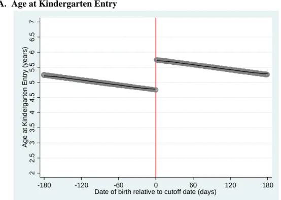
In Figure 1 we explore compliance. In Panel A, we graph the relationship between the
running variable and age in years at school entry. The parametric estimate of the discontinuity is
0.79 years. If compliance were perfect, the gap would be a full year. It is this variation in age at
kindergarten entry that later intersects with compulsory schooling laws and would compel an
9
14
time student to remain in school longer than her older counterparts. In Panel B, we graph the
relationship between a student’s first appearance in kindergarten and her predicted year of
kindergarten entry based on her date of birth. Though the overall redshirting rate (for the entire
analytic sample) was 4.4 percent, students born right to the left of the cutoff are substantially
more likely to be redshirted (by about 18 percentage points). Our overall estimate of redshirting
is in line with national estimates from Bassok and Reardon (2013), who estimate a national
redshirting rate of between 4 and 5.5 percent. In Panel B, as we move leftward along the x-axis
away from the cutoff, the relative age difference shrinks and the likelihood of redshirting
declines.10
The validity of the RD approach rests on the assumption that there is smoothness in the
running variable through the cutoff determining treatment. We test for heaping of births to one
side or the other of the school entry cutoff date using the approach outlined by McCrary (2008)
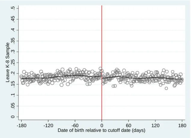
and find no such evidence of birth-date manipulation.11 In Figure 2, we calculate the share of
students that leave our K-8 sample (regardless of whether they later return to the Michigan
data).12 If families of younger students were moving out of Michigan at differential rates, we
might be worried about our choice to begin the high school and college samples with students we
observe around age 14 in our data. But, we find no evidence of differential sample attrition for
students eligible to begin school at a younger age.
10 We conducted a simple descriptive, exploratory analysis of the demographic characteristics of students within ten
days of the school entry cutoff in Figure 2 (i.e., from -10 to 0). We compared average characteristics of the subset of students within that window who delayed kindergarten entry to the characteristics of the subset who started on time. Resultant descriptives confirm patterns uncovered by Bassok and Reardon (2013): Of those who were redshirted, 40 percent were female, 89 percent were white, 5 percent were black, and 40 percent were eligible for free or reduced-price meals. Among those who started on time, 51 percent were female, 64 percent were white, 25 percent were black, and nearly 70 percent were eligible for free or reduced-price meals. Thus, in Michigan, redshirting is a phenomenon more common among male, white, and economically advantaged students.
11 Specifically, we use the “DCdensity” command in Stata developed by McCrary (2008), and find no statistically
significant difference in the density of births at the cutoff.
12
15
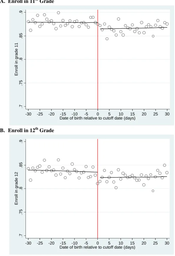
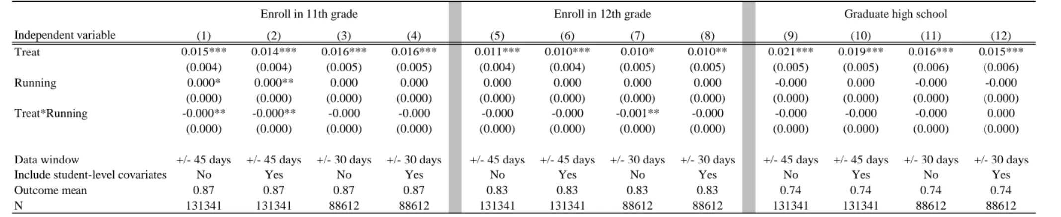
A. Effects on High School Outcomes
We now examine effects of school entry eligibility on our high school attainment
outcomes. Figure 3 presents the graphical depiction of these results while Table 2 reports the
corresponding parametric estimates. On average, we find that students eligible to begin school a
year younger are 1.6 percentage points more likely to enroll in 11th grade, about 1 percentage
point more likely to enroll in 12th grade, and 1.5 percentage points more likely to graduate from
high school than their older counterparts.13 Our effects are slightly larger than those of Dobkin
and Ferreira (2010): In Texas and California, they find effects on high school graduation of 0.8
and 0.9 percentage points, respectively (p. 43). Yet, our results are much closer to those of
Dobkin and Ferreira (2010) than to Cook and Kang’s (2013) finding of a 4 percentage point
difference in rates of completing 12th grade in North Carolina (p. 26).
In addition to attainment, we can explore impacts of this set of laws on academic
performance in high school. All but one of our birth cohorts were required to take the ACT test
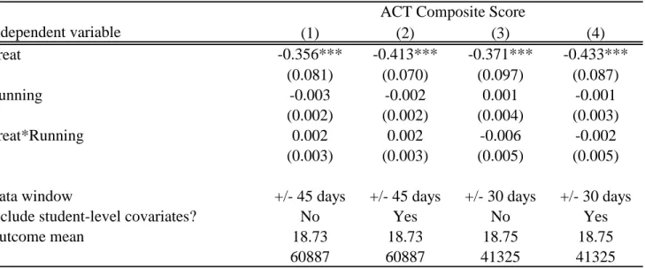
in their penultimate year of high school. Table 3 presents results where the outcome is composite
ACT score, and confirm that students eligible to begin school a year younger score about 0.4
points (i.e., 0.08 standard deviations) lower on the ACT composite (relative to their older
counterparts).14 These achievement results align with Smith (2009) and suggest that the
underperformance of relatively younger students does persist beyond middle school into high
school.15
13 When we nonparametrically estimate the impacts on these same outcomes, we obtain nearly identical point
estimates – all of which are statistically significant at the 10 percent level or lower.
14
We obtain nearly identical results if we exclude the birth cohort of students for whom the ACT was not mandatory at the time they were in 11th grade (i.e., those born in 1989-1990) from our sample.
15 Specifically, these achievement effects are at the lower end of the range of effects on 10th grade performance
16
B. Effects on College Outcomes
We next turn to effects of this same set of laws on measures of postsecondary enrollment,
choice, and persistence. Table 4 presents results for this set of outcomes. Figure 5 presents the
corresponding graphs. We see evidence of a small positive (but statistically insignificant) effect
on overall college-going of less than 1 percentage point. Any small effect on overall college
attendance is driven by statistically significant increases in the likelihood that students first
attend a two-year (rather than four-year) college. Impacts on outcomes that measure whether a
student initially enrolls in a two-year or four-year college suggest that school entry and
compulsory schooling laws affect college choice (i.e., the intensive rather than extensive margin
of college-going). Specifically, students eligible to start school at a younger age are about 2
percentage points more likely to first attend a two-year college and 1.1 percentage points less
likely to first attend a four-year college.16
We also examine the impact of these laws on the total number of college semesters in
which a student enrolls during the three years after her expected, on-time high school graduation.
We estimate that students eligible to begin school at a relatively younger age enroll in about 0.4
fewer semesters of college (of either part- or full-time intensity) than their older counterparts.
This is an unconditional estimate (that is, those who did not attend college receive a value of zero
semesters).
We conclude that students eligible to start school at a relatively younger age are no more
likely to attend (any) college than their older counterparts. Rather, we find evidence that school
entry and compulsory schooling laws shape the college choices of these students. Specifically,
16 In addition, these students are no more likely than their older counterparts to ever attend a four-year. So, the
17
we find that this set of laws shifts the choices of relatively younger college-going students
toward two-year rather than four-year colleges (relative to their older college-going peers). This
finding is in line with Hurwitz et al. (2015) and underscores the need to consider how these
policies shape the college-going trajectories of younger students, especially given recent
evidence on the degree to which the selectivity of a college a student attends shapes her future
welfare (e.g., Hoekstra, 2009; Cohodes & Goodman, 2014).
We also find this set of laws to foster lower levels of postsecondary persistence among
relatively younger students. Perhaps the relative underperformance of younger students in high
school accounts for some of these postsecondary effects. That is, such students are induced to
remain in high school longer, underperform on (mandatory) college entrance exams, and enter
relatively weaker (i.e., two-year) postsecondary institutions. At least, this is one analytic story
that is consistent with the joint results across our high school and college outcomes and with the
Michigan policy context (i.e., the relatively recent adoption of a mandatory, free college entrance
exam in 11th grade). In contrast to the relatively advantaged sample of SAT test-takers studied by
Hurwitz et al. (2015), these postsecondary persistence effects may be more representative of the
impacts of such laws on the broad swath of public school students in a given state.
As a test of the validity of our RD design, we use our student-level covariates (i.e.,
female, white, black, Hispanic, FARM, LEP) as outcomes and present graphical evidence in
Figure 5 on the smoothness of these covariates through the cutoff of interest. In no case do we
estimate a statistically significant discontinuity in any of these student-level covariates at the
cutoff. In addition, we see this same pattern of null results for our other samples (i.e., the high
18
C. Heterogeneity in Impacts by Gender and Economic Advantage
Given past evidence on the differences in impacts of school entry and compulsory
schooling laws by gender and socio-economic advantage, we next explore heterogeneous effects
on our high school and college outcomes by gender and eligibility for free or reduced-price
meals (FARM). Table 5 presents these results.
The results in Table 5 are quite rich and provide considerable nuance to our basic high
school and postsecondary findings. We find that relatively younger students across these four
subgroups underperform on the ACT relative to their older counterparts – but the magnitude of
that underperformance is greater for boys and FARM students. At the same time, while we see
similar positive impacts on high school graduation for boys and girls of the offer to enter school
a year earlier than their slightly older same-gender counterparts, we see substantial differences in
the effect of this offer by FARM eligibility. Specifically, this set of laws induces about 3 percent
more FARM students who are relatively young for grade to graduate from high school,
compared to older FARM students (whereas the impact among non-FARM students is essentially
zero). We therefore conclude that the overall positive impacts on educational attainment through
the end of high school are being almost entirely driven by impacts on socio-economically
disadvantaged students (of both genders).
When we look to heterogeneous effects of school entry and compulsory schooling laws
along the college-going margin, we see that such laws appear to increase college-going among
female and non-FARM students, by 2.7 and 3.1 percentage points respectively – and that these
increases are primarily absorbed by increases within the two-year sector. In contrast, we see little
impact of these laws on the overall college enrollment rates of male and FARM students, but
19
are 2.5 and 1.2 percentage points less likely to first attend a four-year college (relative to a
two-year college). These heterogeneous effects illustrate which groups of students account for the
mix of college (attendance and choice) effects we saw across the full sample. Taken together,
these findings highlight important differences in the impacts of school entry and compulsory
schooling laws on the educational performance and postsecondary pathways of students of
different types.
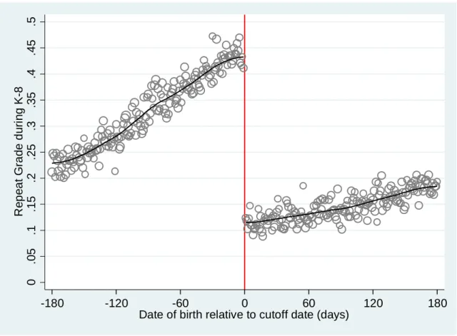
D. Effects on Progression through Elementary and Middle School
Thus far, our analysis provides important information about the net, long-range impacts
of school starting age and compulsory schooling laws. Yet, our high school and college analytic
samples begin with students we can observe in 8th grade. We know from prior literature that
school starting age laws also impact performance and progression in elementary and middle
school. These impacts necessarily shape later outcomes as students age into the time period
where compulsory schooling laws begin to bind. To better understand this phenomenon, we
examine grade progression patterns for students in our K-8 sample who attended school in the
same policy context, just a few years later.
Figure 2 confirmed that leaving the Michigan K-8 data is unrelated to the treatment (i.e.,
the offer to start school a year earlier than one’s peers). Therefore, we drop students who leave
our data from the K-8 analytic sample for this grade progression analysis. Figure 6 examines the
relationship between grade repetition and the age at which children are eligible to start school.
We see a large discontinuity in the likelihood of ever repeating a grade during the K-8 years at
the cutoff. Specifically, students eligible to start school at a relatively younger age are about 30
20
To explore the evolution of this overall impact, we estimate our RD model using the
sample that includes students born within 30 days of either side of the school entry cutoff date on
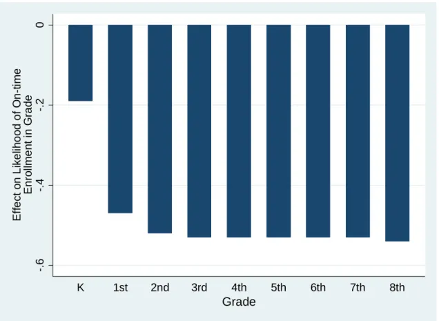
outcomes that measure whether a student is on-time in each grade (K-8). Figure 7 presents these
grade-specific estimates. We base the construction of these on-time outcomes on fist-time
appearance of students in grades. Therefore, the kindergarten bar can be interpreted as the
difference in likelihood of delayed kindergarten entry (i.e., redshirting) for those just to the left
of the cutoff compared to those just to the right. That is, students just barely eligible to start
kindergarten at a relatively younger age are about 18 percentage points more likely to delay
kindergarten entry.
Subsequent bars combine grade retention, grade skipping, and delayed entry into
kindergarten (which puts a student off-track for all subsequent, observed outcomes). As we look
across these bars an interesting pattern emerges– wherein the vast majority of the “ever repeat”
effect is driven by an increased likelihood of repeating kindergarten or first grade. Specifically,
students eligible to start school at a relatively younger age are about 43 percentage point less
likely to enter first grade on time. This effect rises to 47 percentage points by second grade, but
shows little movement between third and eighth grade.17 Thus, this pattern suggests that the
majority of the “grade retention effect” occurs between kindergarten and grade 2. These results
also underscore the fact that effects on our high school and college outcomes are net of the high
rate of K-8 grade repetition among our “treatment” (i.e., relatively younger) students in Michigan.
17
21
We can use our estimate of the increased likelihood of redshirting at the cutoff to
approximate the local average treatment effect (LATE) on our later outcomes of interest. The
LATE provides a better sense of the effects on children who comply with the school entry law.
We do so in the spirit of a two-sample instrumental variables (TSIV) setup (Angrist & Pischke,
2009). First, we assume that the effect we calculate in our K-8 sample would be roughly similar
in our high school and college samples. Second, we use this estimate to scale up the
intent-to-treat (ITT) effects of the offer to start kindergarten at a relatively younger age. For example, if
we focus on one of our postsecondary outcomes that measure college choice, whether a student
first enrolls in a two-year college, we estimate that the effect on compliers is 2.2 percentage
points (i.e., 0.018/0.82). This approximated LATE is in the same ballpark as our estimate of the
ITT effect on the same outcome: 1.8 percentage points.
VII. Conclusions and Policy Implications
In this paper, we exploit the discontinuity in expected legal exposure to K-12 schooling
created by school entry date and students’ exact birth dates to investigate the joint impact of
school entry and compulsory schooling laws on a variety of educational outcomes along the
K-20 pipeline. Using rich administrative data on the universe of public school students in Michigan
over a ten year period, we investigate the effects of being offered kindergarten entry eligibility a
year earlier on high school performance, attainment, and college enrollment, choice, and
persistence. To contextualize these findings, we also explore on-time grade progression from
kindergarten through the 8th grade for one sample of students. Overall, our results provide more
nuanced answers to policy questions about school starting age and compulsory schooling laws in
22
Similar to previous studies in this literature (e.g., Hurwitz et al., 2015; Cook & Kang,
2013; Dobkin & Ferreira, 2010; Bedard & Dhuey, 2006), we find that students eligible to start
school a year earlier (i.e., at a relatively younger age) persist at greater rates into grades 11 and
12, and complete high school at higher rates; yet, these same students demonstrate lower
academic performance while in high school.
Along the postsecondary margin, we find no average effect of these laws on college
enrollment (i.e., the point estimate is positive, small, and statistically insignificant). Yet, for
females and economically advantaged students of both genders who are eligible to start school at
a relatively younger age, we see impacts (of around 3percentage points) on college enrollment.
Yet, the increases in the college-going rates for these subgroups take place entirely within the
two-year college sector. For males and economically disadvantaged students eligible to enroll in
kindergarten at a younger age, this set of laws seems to discourage initial matriculation in a
four-year postsecondary institution, and perhaps dampen the propensity to attend (any) college at all
(i.e., coefficients for these subgroups are negative, small, and statistically significant when the
outcome measures college enrollment along the extensive margin).
We also find that this set of laws fosters lower levels of postsecondary persistence among
students eligible to start school at a relatively younger age. This finding is consistent with
increased enrollment in two-year colleges, where degree and certificate programs are shorter and
student attachment may be weaker than at four-year colleges. While speculative, it is plausible
that the relative underperformance of younger students in high school accounts for some of these
postsecondary effects. Similar to Dobkin & Ferreira (2010), who argue that the net impact of
23
we argue that an additional net impact of these laws is a shift toward (and increased reliance on)
potentially lower-quality postsecondary institutions and lower overall postsecondary persistence.
Yet, the boost in the high school graduation rate of students eligible to start school at a
relatively younger age generated by these laws is a net positive. The fact that this increase is
concentrated among low-income, traditionally disadvantaged students suggests that compulsory
schooling policies are a potentially manipulable policy lever that can be expected to affect
students most at-risk for dropout. Moreover, the fact that some subgroups of relatively younger
students are enrolling in college at higher rates than their older counterparts (e.g., females)
suggests that inducing some students to remain in high school longer may also propel them to
acquire some postsecondary education (that they may have forgone had they been able to drop
out of school sooner). This may be especially true in states like Michigan where all 11th graders
are required to take a college entrance exam. At the same time, the increase in high school
graduation rates among FARM students who are relatively young for grade does not translate
into higher college enrollment rates for this same group. Thus, policies designed to increase high
school graduation among disadvantaged youth may need to be coupled with additional programs
and supports if college access and enrollment are to be expanded for this same population of
students.
Overall, our results present a mixed picture. The differential effects of the combination of
school entry and dropout policies on different subgroups of students suggest that an appropriate
policy response is unlikely to come in the form of shifting school entry policies – after all, under
most feasible school entry schemes, some students will always be relatively younger and others
relatively older. Rather, the interesting take-away from these findings is that the inducement to
24
disadvantaged students in terms of secondary attainment, suggesting that policies aimed at
increasing exposure to schooling for disadvantaged students may increase graduation among this
vulnerable population. At the same time, our findings also illustrate that this set of laws increases
high school graduation rates and college-going rates (within the two-year sector) for girls, but
not for boys or economically disadvantaged students. Therefore, subsequent policy efforts to
smooth and improve transitions from high school to postsecondary education might fruitfully
25
References
Angrist, J. D., & Krueger, A. B. (1991). Does Compulsory School Attendance Affect Schooling
and Earnings? The Quarterly Journal of Economics, 106(4), 979–1014.
Angrist, J. D., & Krueger, A. B. (1992). The Effect of Age at School Entry on Educational Attainment: An Application of Instrumental Variables with Moments from Two Samples.
Journal of the American Statistical Association, 87(418), 328–336.
Bassok, D., & Reardon, S. F. (2013). “Academic Redshirting” in Kindergarten: Prevalence,
Patterns, and Implications. Educational Evaluation and Policy Analysis, 35(3), 283–297.
Bedard, K., & Dhuey, E. (2006). The persistence of early childhood maturity: International
evidence of long-run age effects. Quarterly Journal of Economics, 121(4), 1437-1472.
Black, S. E., Devereux, P. J., & Salvanes, K. G. (2011). Too Young to Leave the Nest? The
Effects of School Starting Age. Review of Economics and Statistics, 93(2), 455–467.
Cohodes, S., & Goodman, J. (2014). Merit aid, college quality and college completion:
Massachusetts' Adams scholarship as an in-kind subsidy. American Economic Journal:
Applied Economics, 6(4), 251-285.
Cook, P. J., & Kang, S. (2013). Birthdays, Schooling, and Crime: New Evidence on the
Dropout-Crime Nexus (Working Paper No. 18791). National Bureau of Economic Research. Retrieved from http://www.nber.org/papers/w18791
Datar, A. (2006). Does Delaying Kindergarten Entrance Give Children a Head Start? Economics
of Education Review, 25(1), 43–62.
Deming, D., & Dynarski, S. M. (2008). The Lengthening of Childhood. Journal of Economic
Perspectives, 22(3), 71–92.
Dobkin, C., & Ferreira, F. (2010). Do school entry laws affect educational attainment and labor
market outcomes? Economics of Education Review, 29(1), 40–54.
Dynarski, S. M., Hemelt, S. W., & Hyman, J. M. (2013). The Missing Manual: Using National
Student Clearinghouse Data to Track Postsecondary Outcomes (Working Paper No. 19552). National Bureau of Economic Research. Retrieved from
http://www.nber.org/papers/w19552
Elder, T. E., & Lubotsky, D. H. (2009). Kindergarten Entrance Age and Children’s
Achievement: Impacts of State Policies, Family Background, and Peers. Journal of
Human Resources, 44(3), 641–683.
Fredriksson, P., & Ockert, B. (2014). Life-cycle effects of Age at School Start. The Economic
26
Hoekstra, M. (2009). The effect of attending the flagship state university on earnings: A
discontinuity-based approach. Review of Economics and Statistics, 91, 171-724.
Hurwitz, M., Smith, J., & Howell, J. S. (2015). Student age and the collegiate pathway. Journal
of Policy Analysis and Management, 34(1), 59-84.
McCrary, J. (2008). Manipulation of the running variable in the regression discontinuity design:
A density test. Journal of Econometrics, 142(2), 698-714.
McCrary, J., & Royer, H. (2006). The Effect of Female Education on Fertility and Infant Health:
Evidence from School Entry Policies Using Exact Date of Birth (Working Paper No. 12329). National Bureau of Economic Research. Retrieved from
http://www.nber.org/papers/w12329
McEwan, P. J., & Shapiro, J. S. (2008). The Benefits of Delayed Primary School Enrollment:
Discontinuity Estimates Using Exact Birth Dates. Journal of Human Resources, 43(1),
1-29
Nichols, A. (2012). RD: Stata module for regression discontinuity estimation. Boston College
Department of Economics. Retrieved from http://ideas.repec.org/c/boc/bocode/s456888.html
Oreopoulos, P. (2013). Should We Raise the Minimum School Leaving Age to Help
Disadvantaged Youth? Evidence from Recent Changes to Compulsory Schooling in the
United States. In J. Gruber (Ed.), An Economic Framework for Understanding and
Assisting Disadvantaged Youth.
Smith, J. (2009). Can Regression Discontinuity Help Answer an Age-Old Question in
Education? The Effect of Age on Elementary and Secondary School Achievement. The
Figure 1. Kindergarten Entry A. Age at Kindergarten Entry
B. Share of On-Time Kindergarten Entrants
Notes: N = 227,417 students; Analytic (K-8) sample excludes special education students. Means are plotted for each day of birth and depicted as hallow circles; the larger the circle, the greater the number of students born on that day. A weighted local polynomial regression of degree zero fits a line on each side of the cutoff using a triangular kernel and a bandwidth of 30 days, where weights are equal to the number of students in each circle.
2 2 .5 3 3 .5 4 4 .5 5 5 .5 6 6 .5 7 Ag e a t Ki n d e rg a rt e n En try (ye a rs)
-180 -120 -60 0 60 120 180
Date of birth relative to cutoff date (days)
0 .1 .2 .3 .4 .5 .6 .7 .8 .9 1 E n rol l O n -T im e in K ind er g ar ten
-180 -120 -60 0 60 120 180
Figure 2. Sample Attrition: K-8 Sample
Notes: N = 227,417 students; Analytic sample excludes special education students. Means are plotted for each day of birth and depicted as hallow circles; the larger the circle, the greater the number of students born on that day. A weighted local polynomial regression of degree zero fits a line on each side of the cutoff using a triangular kernel and a bandwidth of 30 days, where weights are equal to the number of students in each circle.
0
.05
.1
.15
.2
.25
.3
.35
.4
.45
.5
L
ea
v
e K
-8 S
am
p
le
-180 -120 -60 0 60 120 180
Figure 3. Effects of School Entry Eligibility on Educational Attainment in Late High School
A. Enroll in 11th Grade
B. Enroll in 12th Grade
.7
.75
.8
.85
.9
E
n
rol
l in
g
rad
e 11
-30 -25 -20 -15 -10 -5 0 5 10 15 20 25 30 Date of birth relative to cutoff date (days)
.7
.75
.8
.85
.9
E
n
rol
l in
g
rad
e 12
C. Graduate from High School
Notes: N = 88,612 students; All figures use the high school sample. Means are plotted for each day of birth and depicted as hallow circles; the larger the circle, the greater the number of students born on that day. A weighted local polynomial regression of degree zero fits a line on each side of the cutoff using a triangular kernel and a bandwidth of 30 days, where weights are equal to the number of students in each circle.
.7
.75
.8
.85
.9
G
rad
ua
te
h
ig
h
s
c
ho
ol
Figure 4. Effects of School Entry Eligibility on College Attendance, Choice, and Persistence A. Attend College (within 3 years of expected on-time high school graduation)
B. First Attend a Two-Year College
.5
.55
.6
.65
.7
.75
.8
A
tt
en
d c
ol
le
ge
-30 -25 -20 -15 -10 -5 0 5 10 15 20 25 30 Date of birth relative to cutoff date (days)
.2
.25
.3
.35
.4
.45
.5
At
te
n
d
2
-ye
a
r co
lle
g
e
f
irst
C. First Attend a Four-Year College
D. Number of Semesters Enrolled in College (within 3 years of expected on-time high school graduation)
Notes: N = 54,528 students; All figures use the college sample. Means are plotted for each day of birth and depicted as hallow circles; the larger the circle, the greater the number of students born on that day. A weighted local polynomial regression of degree zero fits a line on each side of the cutoff using a triangular kernel and a bandwidth of 30 days, where weights are equal to the number of students in each circle.
.2 .25 .3 .35 .4 .45 .5 At te n d 4 -ye a r co lle g e f irst
-30 -25 -20 -15 -10 -5 0 5 10 15 20 25 30 Date of birth relative to cutoff date (days)
1 1 .5 2 2 .5 3 3 .5 4 Se me st e rs w it h in 3 ye a rs o f ex p ec ted o n-tim e H S g rad ua ti on
Figure 5. Balance of Covariates at Cutoff: College Sample A. Fixed Student Characteristics
B. Time-Varying Student Characteristics
Notes: N = 54,528 students; All graphs are based on the college sample. Means are plotted for each day of birth and depicted as hallow circles; the larger the circle, the greater the number of students born on that day. A weighted local polynomial regression of degree zero fits a line on each side of the cutoff using a triangular kernel and a bandwidth of 30 days, where weights are equal to the number of students in each circle. The y-axes for the fixed student characteristics measure whether a student was ever identified as the outcome within our data.
.25 .3 .35 .4 .45 .5 .55 .6 .65 .7 .75 F em al e
-30 -25 -20 -15 -10 -5 0 5 10 15 20 25 30 Date of birth relative to cutoff date (days)
.5 .55 .6 .65 .7 .75 .8 .85 .9 .95 1 W h ite
-30 -25 -20 -15 -10 -5 0 5 10 15 20 25 30 Date of birth relative to cutoff date (days)
0 .05 .1 .15 .2 .25 .3 .35 .4 .45 .5 B la ck
-30 -25 -20 -15 -10 -5 0 5 10 15 20 25 30 Date of birth relative to cutoff date (days)
0 .05 .1 .15 .2 .25 .3 .35 .4 .45 .5 H is pani c
-30 -25 -20 -15 -10 -5 0 5 10 15 20 25 30 Date of birth relative to cutoff date (days)
.25 .3 .35 .4 .45 .5 .55 .6 .65 .7 .75 F A RM
-30 -25 -20 -15 -10 -5 0 5 10 15 20 25 30 Date of birth relative to cutoff date (days)
0 .05 .1 .15 .2 .25 .3 .35 .4 .45 .5 LE P
Figure 6. Effect of School Entry Eligibility on Grade Repetition: K-8 Sample
Notes: N = 186,085 students; Analytic (K-8) sample excludes special education students as well as students who leave the data (i.e., Michigan public schools). Means are plotted for each day of birth and depicted as hallow circles; the larger the circle, the greater the number of students born on that day. A weighted local polynomial regression of degree zero fits a line on each side of the cutoff using a triangular kernel and a bandwidth of 30 days, where weights are equal to the number of students in each circle.
0
.05
.1
.15
.2
.25
.3
.35
.4
.45
.5
R
e
pe
at
G
rad
e du
ri
n
g K
-8
-180 -120 -60 0 60 120 180
Figure 7. Effect of School Entry Eligibility on Timely Progression through Elementary and Middle School
Notes: N = 29,624 students; Analytic (K-8) sample excludes special education students as well as students who leave the data (i.e., Michigan public schools). Each bar represents a separate effect estimated using a parametric RD model on a window of data that includes 30 days on each side of the cutoff.
-.
6
-.
4
-.
2
0
E
ff
ec
t
o
n Li
k
el
ih
oo
d of
O
n-ti
m
e
E
n
rol
lm
e
nt
i
n
G
ra
de
K 1st 2nd 3rd 4th 5th 6th 7th 8th
Table 1. Descriptive Statistics by Sample
A. Postsecondary Sample (Born 1989 - 1992)
Data window Variable Mean Standard Deviation Mean Standard Deviation Mean Standard Deviation
Female 0.49 0.50 0.49 0.50 0.49 0.50
White 0.72 0.45 0.71 0.45 0.71 0.45
Black 0.24 0.42 0.24 0.43 0.24 0.43
Hispanic 0.02 0.16 0.02 0.16 0.02 0.15
Other 0.01 0.11 0.01 0.11 0.01 0.12
FARM 0.51 0.50 0.52 0.50 0.52 0.50
LEP 0.02 0.13 0.02 0.13 0.02 0.13
N
B. High School Sample (Born 1989 - 1994)
Data window Variable Mean Standard Deviation Mean Standard Deviation Mean Standard Deviation
Female 0.49 0.50 0.49 0.50 0.49 0.50
White 0.72 0.45 0.71 0.45 0.71 0.45
Black 0.23 0.42 0.24 0.43 0.24 0.43
Hispanic 0.03 0.16 0.03 0.16 0.03 0.16
Other 0.02 0.15 0.02 0.15 0.02 0.15
FARM 0.54 0.50 0.55 0.50 0.55 0.50
LEP 0.02 0.14 0.02 0.15 0.02 0.14
N
C. K-8 Sample (Born 1997 - 1999)
Data window Variable Mean Standard Deviation Mean Standard Deviation Mean Standard Deviation
Female 0.49 0.50 0.49 0.50 0.49 0.50
White 0.69 0.46 0.68 0.46 0.69 0.46
Black 0.20 0.40 0.20 0.40 0.20 0.40
Hispanic 0.06 0.24 0.06 0.24 0.06 0.24
Other 0.05 0.21 0.05 0.22 0.05 0.22
FARM 0.62 0.49 0.62 0.48 0.63 0.48
LEP 0.08 0.27 0.08 0.27 0.08 0.27
N
88612 131341
363588
+/- 30 days +/-45 days
+/- 120 days
+/- 30 days +/- 45 days
+/- 120 days
54528 80971
224855
Notes: Samples exclude special education students. See text for additional sample-specific construction details.
38220 56848
155893
+/- 30 days +/- 45 days
Table 2. Effects of School Entry Eligibility on Educational Attainment through High School
Independent variable (1) (2) (3) (4) (5) (6) (7) (8) (9) (10) (11) (12) Treat 0.015*** 0.014*** 0.016*** 0.016*** 0.011*** 0.010*** 0.010* 0.010** 0.021*** 0.019*** 0.016*** 0.015***
(0.004) (0.004) (0.005) (0.005) (0.004) (0.004) (0.005) (0.005) (0.005) (0.005) (0.006) (0.006) Running 0.000* 0.000** 0.000 0.000 0.000 0.000 0.000 0.000 -0.000 0.000 -0.000 -0.000 (0.000) (0.000) (0.000) (0.000) (0.000) (0.000) (0.000) (0.000) (0.000) (0.000) (0.000) (0.000) Treat*Running -0.000** -0.000** -0.000 -0.000 -0.000 -0.000 -0.001** -0.000 -0.000 -0.000 -0.000 0.000
(0.000) (0.000) (0.000) (0.000) (0.000) (0.000) (0.000) (0.000) (0.000) (0.000) (0.000) (0.000)
Data window +/- 45 days +/- 45 days +/- 30 days +/- 30 days +/- 45 days +/- 45 days +/- 30 days +/- 30 days +/- 45 days +/- 45 days +/- 30 days +/- 30 days Include student-level covariates No Yes No Yes No Yes No Yes No Yes No Yes Outcome mean 0.87 0.87 0.87 0.87 0.83 0.83 0.83 0.83 0.74 0.74 0.74 0.74 N 131341 131341 88612 88612 131341 131341 88612 88612 131341 131341 88612 88612
Enroll in 12th grade
Enroll in 11th grade Graduate high school
Table 3. Effects of School Entry Eligibility on Academic Achievement in High School
Independent variable (1) (2) (3) (4)
Treat -0.356*** -0.413*** -0.371*** -0.433***
(0.081) (0.070) (0.097) (0.087)
Running -0.003 -0.002 0.001 -0.001
(0.002) (0.002) (0.004) (0.003)
Treat*Running 0.002 0.002 -0.006 -0.002
(0.003) (0.003) (0.005) (0.005)
Data window +/- 45 days +/- 45 days +/- 30 days +/- 30 days
Include student-level covariates? No Yes No Yes
Outcome mean 18.73 18.73 18.75 18.75
N 60887 60887 41325 41325
ACT Composite Score
Table 4. Effects of School Entry Eligibility on College Attendance, Choice, and Persistence
Independent variable (1) (2) (3) (4) (5) (6) (7) (8) (9) (10) (11) (12) (13) (14) (15) (16)
Treat 0.014 0.012 0.008 0.007 0.026*** 0.026*** 0.019** 0.018** -0.013** -0.014** -0.011 -0.011* -0.343*** -0.354*** -0.375*** -0.378*** (0.008) (0.007) (0.010) (0.009) (0.007) (0.007) (0.008) (0.008) (0.006) (0.006) (0.008) (0.007) (0.044) (0.037) (0.053) (0.045) Running 0.000 0.000 -0.000 0.000 -0.000 -0.000 -0.001 -0.001 0.000* 0.000** 0.001* 0.001** 0.001 0.002 -0.000 0.000
(0.000) (0.000) (0.000) (0.000) (0.000) (0.000) (0.000) (0.000) (0.000) (0.000) (0.000) (0.000) (0.001) (0.001) (0.002) (0.002) Treat*Running -0.000 -0.000 -0.001 -0.000 0.000 0.000 0.000 0.000 -0.001** -0.001*** -0.001** -0.001* -0.005*** -0.005*** -0.005* -0.004* (0.000) (0.000) (0.001) (0.000) (0.000) (0.000) (0.000) (0.000) (0.000) (0.000) (0.000) (0.000) (0.002) (0.001) (0.003) (0.002)
Data window +/- 45 days +/- 45 days +/- 30 days +/- 30 days +/- 45 days +/- 45 days +/- 30 days +/- 30 days +/- 45 days +/- 45 days +/- 30 days +/- 30 days +/- 45 days +/- 45 days +/- 30 days +/- 30 days
Include student-level covariates? No Yes No Yes No Yes No Yes No Yes No Yes No Yes No Yes
Outcome mean 0.55 0.55 0.55 0.55 0.29 0.29 0.29 0.29 0.27 0.27 0.27 0.27 2.46 2.46 2.45 2.45
N 80971 80971 54528 54528 80971 80971 54528 54528 80971 80971 54528 54528 80971 80971 54528 54528
Notes: "Treat" is an indicator that denotes whether a student is eligible to start school at a relatively younger age. All models include cohort fixed effects. Standard errors clustered on day of birth appear in parentheses: *** p<0.01, ** p<0.05, *p<0.1.
Enroll in college (within 3 years of expected on-time
high school graduation) First enrollment is in a 2-year college First enrollment is in a 4-year college
Table 5. Heterogeneous Effects of School Entry Eligibility on High School Performance and Educational Attainment: by Gender and Poverty Status
Subgroup
Outcome (1) (2) (3) (4) (5) (6) (7) (8)
High School Outcomes
Enroll in 11th grade 0.010* 0.011* 0.018*** 0.021*** 0.024*** 0.029*** 0.003 0.001
(0.005) (0.007) (0.005) (0.006) (0.006) (0.008) (0.003) (0.004)
Enroll in 12th grade 0.007 0.007 0.014** 0.014** 0.017*** 0.018** 0.003 0.001
(0.006) (0.007) (0.005) (0.006) (0.006) (0.008) (0.004) (0.005)
Graduate high school 0.022*** 0.020** 0.016** 0.012 0.030*** 0.026*** 0.006 0.003
(0.007) (0.008) (0.007) (0.008) (0.007) (0.009) (0.005) (0.007)
ACT Composite Score -0.284*** -0.349*** -0.423*** -0.514*** -0.487*** -0.404*** -0.325*** -0.457***
(0.108) (0.115) (0.097) (0.120) (0.091) (0.112) (0.110) (0.128)
Postsecondary Outcomes
Enroll in college 0.027** 0.027* -0.003 -0.012 -0.002 -0.014 0.028*** 0.031***
(0.011) (0.014) (0.010) (0.012) (0.010) (0.013) (0.009) (0.011)
Enroll in 2-yr college first 0.030*** 0.024* 0.022** 0.013 0.011 -0.002 0.042*** 0.041***
(0.010) (0.013) (0.009) (0.011) (0.010) (0.013) (0.010) (0.011)
Enroll in 4-yr college first -0.004 0.003 -0.024*** -0.025*** -0.014** -0.012* -0.014 -0.011
(0.009) (0.011) (0.008) (0.009) (0.006) (0.007) (0.010) (0.012)
Number of semesters enrolled -0.295*** -0.330*** -0.412*** -0.425*** -0.172*** -0.202*** -0.546*** -0.569***
(0.060) (0.075) (0.048) (0.057) (0.043) (0.051) (0.053) (0.062)
Data window +/- 45 days +/- 30 days +/- 45 days +/- 30 days +/- 45 days +/- 30 days +/- 45 days +/- 30 days
N (high school sample) 64214 43240 67127 45372 71893 48389 59448 40223
N (college sample) 39437 26585 41534 27943 42125 28286 38846 26242
Non-FARM
Female Male FARM