Proper shape representation of single figure and multi-figure anatomical objects

(1)

Proper Shape Representation of Single Figure and

Multi-Figure Anatomical Objects

Qiong Han

A dissertation submitted to the faculty of the University of North Carolina at Chapel Hill in partial fulfillment of the requirements for the degree of Doctor of Philosophy in the Department of Computer Science.

Chapel Hill 2008

Approved by:

Stephen M. Pizer, Advisor

Edward L. Chaney, Reader

Sarang Joshi, Reader

James N. Damon, Committee Member

Keith Muller, Committee Member

(2)

c

2008

Qiong Han

(3)

Abstract

Qiong Han: Proper Shape Representation of Single Figure and Multi-Figure Anatomical Objects

(Under the direction of Stephen M. Pizer)

Extracting anatomic objects from medical images is an important process in various medical applications. This extraction, called image segmentation, is often realized by deformable models. Among deformable model methods, medial deformable models have the unique advantage of representing not only the object boundary surfaces but also the object interior volume.

Based on one medial deformable model called the m-rep, the main goal of this dis-sertation is to provide proper shape representations of simple anatomical objects of one part and complex anatomical objects of multiple parts in a population. This dissertation focuses on several challenges in the existing medially based deformable model method: 1. how to derive a proper continuous form by interpolating a discrete medial shape rep-resentation; 2. how to represent complex objects with several parts and do statistical analysis on them; 3. how to avoid local shape defects, such as folding or creasing, in shapes represented by the deformable model. The proposed methods in this dissertation address these challenges in more detail:

1. An interpolation method for a discrete medial shape model is proposed to guaran-tee the legality of the interpolated shape. This method is based on the integration of medial shape operators.

(4)

(5)

Acknowledgments

First and foremost, I want to thank Steve Pizer, for his support and guidance. His almost ”contagious” passion in our research of the Medical Image Display and Analysis Group (MIDAG) partially contributes to the existence of this dissertation. My thanks also go to Ed Chaney, who provided the important driving problems for this dissertation, Jim Damon, who taught me the medial mathematics in great detail, Sarang Joshi, who guided me on the work of the multi-figure m-rep, Keith Muller, who suggested a systematic way to conduct an evaluation, starting from a well designed test sample, and Jack Snoeyink, who helped me on writing this document.

I feel fortunate to work in the MIDAG. The support provided by Graham Gash and Gregg Tracton has been impeccable. I also want to thank Guido Gerig, Mark Styner, Julian Rosenman, and all my former colleagues in the MIDAG, especially Andrew Thall, Thomas Fletcher, Ja-Yeon Jeong, Xiaoxiao Liu, Derek Merck, and Rohit Saboo. The discussions with you, the comments from you, the opportunity to shadow you around have all become valuable pieces in my life as a graduate student in Chapel Hill.

I also want to thank Janet Jones and Timm Quigg for their help when I needed it the most.

(6)

List of Tables

(10)

List of Figures

1.1 Anatomical objects with multiple named parts . . . 5

2.1 The internal and end medial atom in a discrete m-rep . . . 25

2.2 An object with two parts represented by a two-figure m-rep. . . 32

3.1 Demonstration of the interpolated spoke fields from a discrete m-rep . . . 53

3.2 Interpolation of end medial atoms . . . 63

3.3 Interpolation results on synthetic ellipsoid m-reps and on real-patient kidney m-reps . . . 67

4.1 Multi-part anatomical objects with protrusion or indentation subparts . . 71

4.2 Parameterizations of a single figure m-rep . . . 73

4.3 Demonstration of hinge geometry . . . 75

4.4 Demonstration of the medial sheet for a blend region . . . 88

4.5 Demonstration of two interpolated multi-figure m-reps . . . 89

4.6 The accumulated sum of the variances from global statistics PGAg and demonstration of hierarchical statistics . . . 92

5.1 Illegal local shape defects: folding and creasing . . . 95

5.2 Demonstration of the shape effect of λri values and demonstration of a sample illegality function . . . 100

5.3 Warped ellipsoids and fitting results . . . 104

5.4 Sample fitted models from fittings without and with using the illegality penalty . . . 106

(11)

6.1 Comparison results of warped ellipsoids shown in terms of the average surface distance and the Dice coefficient . . . 114

6.2 Comparison results of sampled kidney m-reps shown in terms of the av-erage surface distance and the Dice coefficient . . . 114

6.3 Diagram flow to lay out the evaluate of multi-figure m-rep fitting . . . . 119

(12)

Chapter 1 Introduction

1.1 Motivation

Medical image processing is becoming an important component in modern medicine because it assists physicians in diagnosing and treating diseases. The following list shows some medical image processing applications:

• Computer-assisted nodule detection in chest CT images helps physicians to screen

for early-stage lung cancer, which significantly increases the survival rate of pa-tients with early-stage lung cancer;

• Statistical shape analysis applied to neurological images sheds light on early

diag-nosis of children with autism;

• Image-guided radiation therapy (IGRT) helps radiation oncologists to locate

tu-mors and organs at risk more precisely and plan better radiation treatment plans.

(13)

geometric shape models and deforming shape models into target images via object shape and object-relative image intensity (appearance) information inferred from a population of anatomical objects. The use of the inferred information from a population enables deformable model methods to deal with challenging images, in which noise is apparent or contrast across object boundaries is lacking. The second task, statistical shape anal-ysis, applies learned shape statistics on two populations of shapes to infer differences between the populations, e.g., by hypothesis testing.

Both tasks require the understanding of object shapes or appearance in one or more populations. This is achieved by learning object shape or appearance variations of a training set of anatomical objects from a respective object population. There are two common approaches to use a set of training objects: 1. estimating shape or appearance probability distributions from training objects or images from a population and then computing the estimated probability on a new object for statistical shape analysis or on a new image for image segmentation; 2. using the training set of anatomical objects to solve problems without learned shape or appearance probability distributions. The first approach is often used in posterior optimization for image segmentation or Bayesian clas-sification, and the second approach is used in shape discrimination, via support vector machine (SVM) or distance weighted discriminant methods [Vapnik (1993)]. This disser-tation focuses on the first approach, which summarizes shape and appearance statistics from a training set of objects and applies the estimated probability distributions to a new object.

(14)

two populations. Our experiences indicate that quality of the shape and appearance statistics is crucial to the success of both image segmentation and shape analysis tasks. Shape statistics are learned from shape parameters of a set of pre-extracted shape models. Appearance statistics are learned from shape-relative volumetric regions around shape boundaries. How the shapes are represented directly affects how shape and ap-pearance information is obtained for each training object. Therefore the quality of both shape and appearance statistics depends on the quality of the shape models.

Various shape model representations [Cootes et al. (1995); Pizer et al. (2003); Styner et al. (2006); Yang et al. (2003)] have been proposed for anatomical objects, with model-ing an object population as the goal in mind. In particular, the UNC MIDAG group has developed a discrete medial shape representation called the m-rep [Pizer et al. (2003)] that is especially suited to this population modeling task: discrete m-reps have local-ized shape control allowing accurate and precise representation of anatomical structures; discrete m-reps can represent objects with a fixed topology from a population and can capture non-linear shape variations in these objects via learned shape statistics [Fletcher (2005)]. However, the following challenges still remain:

1. Undesired shape defects, such as creasing, can not be efficiently prevented;

2. Objects with more than one component, such as a liver with two lobes, are only represented as a whole, not in terms of its components;

3. Interpolation within discrete medial shape models is not well understood and im-plemented.

(15)

1.1.1 Proper Shape for Population Modeling

Any undesired shape defects in training shape models are unnatural shape features, such as local creasing or folding. These shape defects will be reflected in inferred statistics based on those models. The ”tainted” statistics will yield undesirable results.

Shape representations in deformable model methods provide not only the geomet-ric basis to infer shape statistics but also the object-relative coordinates via which the image intensities are extracted to infer appearance statistics. A shape representation that guarantees shapes as legal or proper, i.e. free of any local creasing and folding, are necessary to obtain both good shape and good appearance statistics. These shape and appearance statistics are used as priors and likelihoods, respectively, in image segmen-tations, via posterior optimization on deformable models. Shape statistics are also used in statistical shape analysis applications such as hypothesis testing. Shape legality is thus important to the success of image segmentation using posterior optimization and statistical shape analysis.

(16)

Figure 1.1: a) A prostate with two seminal vesicle protrusions. b) A liver represented by the union of the left and right lobes. Object a has three single-figure parts while object b has two such parts.

1.1.2 Multi-part Objects

Shape representation and statistics of simple one-part objects have been widely stud-ied. Methods using various representations have been proposed and shown to be effective [Cootes et al. (1995); Fletcher et al. (2004); Yang et al. (2003)]. However, many anatom-ical objects have multiple named parts. For example, a prostate (Figure 1.1-a) has two seminal vesicles attached to it, and a liver (Figure 1.1-b) has both left and right lobes. The difficulty of representing multi-part objects lies in the fact that only modeling each individual part is not sufficient. The inter-relations among parts have been elusive for boundary based shape representations. The inter-relations include part-to-part con-nection, global deformations to all the connected parts, and implied deformations from one part to an adjacent part.

Due to the inherent complexity of objects with multiple parts, previous shape and statistical descriptions of such objects concentrated on their global structures [Cootes et al. (1995); Gerig et al. (2001)] or on the extremely local behavior of geometric prim-itives, such as points, without references to the parts’ inter-relations [Csernansky et al. (1998); Styner et al. (2003)].

(17)

Medially based shape representations parameterize both the object interior and the adjacent exterior volumetric regions. This allows us to model the relations between pairs of adjacent object parts because each part can be known in the local coordinates of its connected neighboring part. The local coordinates also allow us to describe the inter-part relations by a small set of parameters. This makes it feasible to explicitly model multi-part objects as a connected set of parts [Han et al. (2004)] and to conduct hierarchical statistical analysis on the parts of the objects from a population [Han et al. (2005)].

1.1.3 Interpolation of Discrete Medial Representations

A parametric shape representation captures an object shape via continuous functions of arguments on topologically equivalent shapes. For shapes with spherical topology, an example is a shape representation based on piece-wise polynomial splines or a shape rep-resentation based on Fourier basis functions [Duncan (1992); Staib and Duncan (1996)] that globally represents an object shape with a set of parameters as the coefficients of the basis functions. Such representations, however, do not provide a means to model localized shape variations.

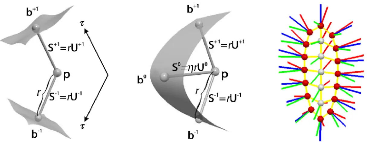
A discrete medial shape representation, such as a discrete m-rep, is composed of a set of discrete medial samples, called medial atoms [Pizer et al. (2003)]. Each medial atom has a hub position point and two to three spoke vectors from the hub position to the boundary points, as shown in figure 2.1. Although the discrete m-rep does not give a continuously parameterized representation of the object, it conveniently provides localized control over the object shape. By interpolating or approximating the set of discrete primitives, we can have a continuous and parameterized representation derived from the discrete object, and we can still benefit from capturing the localized shape variations by the discrete primitives.

(18)

as a 3D point, r is the radius or the length of spokes, and U+1,−1 are the directions of the spokes (more detail about medially based representations can be found in section 2.1). An interpolation or approximation of (p, r,U+1,−1) can provide a parameterized medial representation (p(u, v), r(u, v),U(u, v)+1,−1_{). In order for the interpolated atoms} to stay medial [Blum and Nagel (1978)], the interpolated or approximated atoms must satisfy a set of constraints as follows:

1. The bisector spoke of each atom is tangential to the medial sheet surface formed byp(u, v) at the point of which the atom hub p lies;

2. The normal of the medial sheet surface is in the direction of the difference vector between the pair of spokes in a medial atom;

3. The derivatives of the spoke along the medial sheet and the medial sheet surface fulfill certain conditions to keep the spokes from crossing one another.

Although interpolation of points in R3 has been well studied, a new interpolation

method is needed for medial atoms because the interpolated medial atoms must fulfill the set of constraints above. In particular, each discrete medial primitive, i.e., each medial atom lies in a curved Riemannian space, and the dimensions of each atom are not independent because its spoke directions must reflect the derivatives of the medial sheet surface and of the radius field on the medial sheet. There has not been an interpolation method on discrete m-reps that fulfill such constraints. A method to interpolate m-rep atom hubs into a smooth medial sheet surface and to interpolate m-rep spokes into a smooth spoke field is proposed in this dissertation. The key is to maintain the relation among all the atom dimensions so the legality of the interpolated medial sheet and spoke fields on the sheet is upheld.

(19)

represent the shape variations in the population by shape statistics. Shape representa-tions using dense boundary points have already approached this correspondence problem via an interpolation of boundary points [Davies et al. (2002); Gerig et al. (2001)]. The improvement to the correspondence across objects represented by m-reps relies on this proposed interpolation method in this dissertation.

Complex objects, such as livers with more than one component, are more challeng-ing to represent. This dissertation will propose a means to represent such objects by establishing a hierarchy of connected parts. The connection between each pair of object parts also requires interpolations, and this dissertation will propose a method for such interpolation by a similar interpolation scheme as that within a medially represented object part.

This dissertation thus concentrates on proper shape representations of anatomical objects, including simple objects and complex objects with multiple parts, based on an interpolation method of medial spokes.

1.2 Thesis Objectives and Claims

Thesis claim: An interpolation method, based on sound mathematics, and the hinge ge-ometry, defining the interrelations between connected object parts, provide a powerful tool to derive a medial representation of both single part and multi-part objects from dis-crete m-reps. When incorporated with explicit geometric constraints, based on the same mathematics, the shape models based on discrete m-reps guarantee proper shape repre-sentations of both single and multi-part objects. These shapes allow statistical modeling of both shape and appearances in a population.

The contributions of this dissertation are as follows:

• A method to interpolate a discrete medial model into a continuously parameterized

(20)

• A description of geometric interrelations among adjacent parts for an object with

multiple parts

• A means to calculate hierarchical statistics of an object of multiple parts, from

the global level to the local level of each parts and their interrelations

• An explicit use of an illegality penalty in binary fitting to improve the

smooth-ness of fitted shapes, thereby leading to properly trained shape and appearance statistics and eventually better segmentation results

• A way to generate standard test cases of deformable m-reps via synthesizing

warped ellipsoids or via sampling learned shape space

1.3 Dissertation Outline

The rest of my dissertation is organized as follows.

Chapter 2 reviews the related background literature including deformable model methods in general for modeling a population of objects, medially based shape repre-sentations, and the mathematics for medial structures.

Chapter 3 details the interpolation method on a medial shape representation. For single part objects, the interpolation is applied to internal and end primitives. For objects with multiple parts, the interpolation is based on the interpolation of each part, with smooth transitions between each pair of adjacent parts generated via so-called spoke interpolation.

Chapter 4 describes the representation of objects with multiple parts in detail, in-cluding the definition of the interrelations among object parts, the coordinate system to describe that interrelations, part deformation implied by adjacent part, and self-deformation of parts without affecting adjacent parts.

(21)

legality constraints in the binary fitting process of fitting a template model into target binary images.

(22)

Chapter 2 Background

As the driving task of this dissertation, medical image segmentation is the process of delineating anatomical structures from the background in an image. Segmenting anatomical objects from a medical image containing information of complex anatomical structures, already a challenge, is made even more difficult by image noise, sampling artifacts, lack of contrast at object boundaries, and neighboring anatomical structures with confusing intensities.

(23)

2.1 Deformable Model Methods

Early segmentation methods, such as the one proposed in [Marr and Nishihara (1978)], used local image features such as edges and corners to construct a shape model in a bottom-up fashion. Local edge or corner detectors applied to an image can, however, produce false edges or gaps. These false edges can become parts of a segmented object boundary that do not exist in a real anatomical object; these false gaps can distort or break a segmented boundary. Such a problem can be overcome by incorporating larger scale information in the image or a global model of the target object. Although such information has been used for boundary delineation via grouping, labeling, and scale-space analysis in [Kass et al. (1988)], this method did not guarantee finding a complete object boundary. Furthermore, these early segmentation methods were mostly applied to 2D image slices and are conceptually and computationally expensive to extend to 3D. Where the local feature based methods fail is exactly where deformable model meth-ods [McInerney and Terzopoulos (1996); Caselles et al. (1997)] shine. Deformable model methods use information gathered from different scale levels. Recent deformable model methods use learned shape probability distributions to guide their segmentation process. In general, deformable model methods segment images in a top-down fashion, which is more likely to find the global optimal object boundary in an efficient way.

Deformable model methods can be categorized by their model representations and the means by which their image segmentation, i.e., the process of fitting a template model into a target image, is conducted.

Among deformable model representations, the point distribution model (PDM) [Dry-den and Mardia (1998); Kass et al. (1988)] using a set of landmarks is among the earliest. Numerous boundary points formed landmarks in the shape representations of later meth-ods, such as the active shape model (ASM) [Cootes et al. (1995)] and active appearance model (AAM) [Cootes et al. (2001)] methods.

(24)

onto orthogonal functions. They represent object boundaries by the coefficients of or-thogonal basis functions. Choices of the oror-thogonal basis functions include sinusoidal functions [Duncan (1992)] and spherical harmonic functions [Gerig et al. (2001)].

There are also deformable model methods using medially based shape representa-tions, including the ones following Blum’s notation for medial axis [Blum and Nagel (1978)], such as in [Yushkevich et al. (2003); Terriberry et al. (2007)], and the discrete m-rep method [Pizer et al. (2003)], in which each shape representation primitive is the combination of a sample from a Blum medial axis and extra components.

These deformable model methods use quite different shape representations. They also approach the image segmentation problem differently. The earlier deformable model methods [Dryden and Mardia (1998); Kass et al. (1988)] segment medical images by deforming a template model M into an image I via optimizing an objective function summing two terms: image match Fimg and geometric typicality Fgeom. The image

match term Fimg measures how a deformed model M0 fits into a given target image

I, and the geometric typicality term penalizes peculiar shapes with creased or folded surfaces to prevent or reduce shape defects in a fit shape model. I call this type of deformable model methods the geometric type.

To guide their segmentation process, recent deformable model methods [Cootes et al. (1995); Mitchell et al. (2002); Pizer et al. (2003)] use learned probability distributions of both shape and appearance, i.e., image intensity relative to the object model. Based on the Bayes’ theorem [Bayes (1958)], the posterior probabilityp(M|I) can be factored into two terms: the shape prior p(M) and the image likelihood p(I|M), shown in equation 2.1, where p(I) is the marginal probability of a given image and is constant for a given M:

logp(M|I) = logp(M)p(I|M)

p(I) = logp(M) + logp(I|M)−log(I) (2.1)

(25)

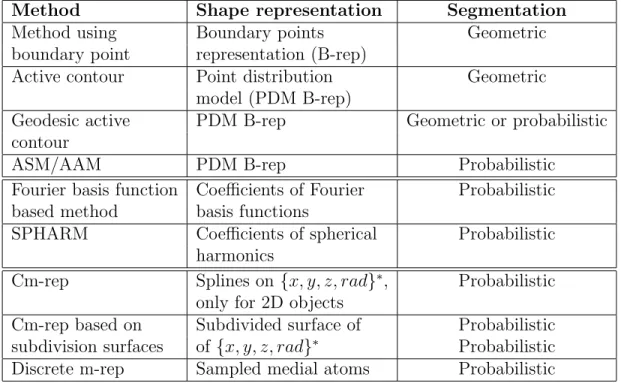
Method Shape representation Segmentation

Method using Boundary points Geometric

boundary point representation (B-rep)

Active contour Point distribution Geometric model (PDM B-rep)

Geodesic active PDM B-rep Geometric or probabilistic contour

ASM/AAM PDM B-rep Probabilistic

Fourier basis function Coefficients of Fourier Probabilistic based method basis functions

SPHARM Coefficients of spherical Probabilistic harmonics

Cm-rep Splines on {x, y, z, rad}∗, Probabilistic only for 2D objects

Cm-rep based on Subdivided surface of Probabilistic subdivision surfaces of {x, y, z, rad}∗ _{Probabilistic}

Discrete m-rep Sampled medial atoms Probabilistic

Table 2.1: Categorization of deformable model methods. ∗ rad indicates a radius scalar field on the 3D surface {x, y, z}

model methods within such a framework segment an image by optimizing the posterior probability, calculated as the sum of the shape prior and image likelihood terms from the learned shape and appearance statistics. I call such group of deformable model methods the probabilistic type.

The geometric type of deformable model methods is still widely used to extract shape models for learning shape and appearance statistics, because no shape or appear-ance statistics are available at this step of learning. However, the probabilistic type of deformable model methods are used to crack the most difficult image segmentation problem using the learned probability distributions.

(26)

2.1.1 Active Contour and Geodesic Active Contour Methods

The discrete active contour model, also known as the snake, was first proposed by Kass, et al. in [Kass et al. (1988)]. The method is named ”snake” because the way an active contour deforms resembles the movement of a snake.

An active contourVis a set of verticesp_i on an object boundary. An energy function is defined for V with two parts (shown in 2.5) that the authors of [Kass et al. (1988)] called the internal and external part, which respectively correspond to the geometric typicality term and image match term in an objective function for the geometric type of deformable model methods.

E(V) = αEint(V) +βEext(V); (2.2)

Eint(V) = γEcontinuity(V) +δEballoon(V); (2.3)

Eext(V) = ηEintensity(V) +φEgradient(V); (2.4)

The internal energy Eint, i.e., the geometric typicality term, enforces V to stay

smooth and propagate in a desired direction. There are two sub-terms in Eint: the

continuity (or smoothness) term and the balloon force term. The weight γ for the continuity term controls the smoothness of a deformed contour V0. If γ is too big, the resulting contour V0 will be over-smoothed and fail to fit into the image well enough; if γ is too small, V0 will be too jaggy with sharp features such as corners. The balloon force term ensures that a snake curve keeps propagating in a desired direction, either expanding or shrinking depending on the specific target object. These two internal energy terms force a snake curve to propagate smoothly regardless of the image intensity information.

The external energy Eext, i.e., the image match term, depends on the neighboring

(27)

to a region of low or high image intensities; Egradient attracts V to edges in an image.

The key is that the direction of the image gradient at an object boundary point should be similar to the unit normal direction of the active contour at that same point. In practice, for noisy images, geometry-limited diffusion [Whitaker (1993)] helps V to converge to the correct boundary at appropriate image scales.

In a continuous form of the energy function for active contours, the energy terms

Eint and Eext are both integrals of local energy measures on the contour parameterized

byq:

E(V) =α

Z 1

0

(eint(V(q)))dq+

Z 1

0

(eext(V(q)))dq (2.5)

where the integrand in the first term eint corresponds to the local internal energy at the

contour pointV(q), i.e., the geometric typicality term, and the integrand in the second term eext corresponds to the local external energy there, i.e., the image match term.

Geometric models of active contours using the continuous form of the energy func-tions were proposed in [Malladi et al. (1995)]. Their method is based on the theory of curve evolution and geometric flow. E(V) sums two terms: one related to the regu-larity of the contour curve and the other related to the shrinking or expanding of the contour towards object boundaries. Their method is driven by mean curvature flow, implemented by solving partial differential equations (PDEs). Different from the energy minimization process in the original snake method, the geometric active contours allow automatic changes in the shape topology if implemented by level-sets [Kimmel et al. (1995)]. As a result, multiple objects can be segmented simultaneously without any pre-knowledge of a given image. This is arguably both the strength and weakness of a geometric active contour method: it can segment multiple objects without guidance but can also undesirably break a single object into multiple parts in the presence of image artifacts.

(28)

i.e., minimal distance curves, the geodesic active contour method proposed in [Caselles et al. (1997)] further pushed forward the methods in the active contour category. This geodesic approach allows the connection of classical snake methods based on energy minimization to geometric active contour methods based on curve evolution theory. The geodesic contour method improves the geometric active contour methods by the use of a new velocity term based on image appearance, allowing stable boundary detection when image gradients suffer from large variations, e.g., gaps in image edges.

The deformable model methods in the active contour category share the same vertex point based shape representation. These methods solely depend on local geometry and image features, making them both efficient for image segmentations and sensitive to local image defects, which might lead to undesired leaking of the contours or being stuck at local sub-optimal solutions.

Attempts have been made to integrate global shape priors into these active contour based methods [Yang et al. (2003)]. The proposed method applies principal component analysis (PCA), a linear statistical analysis method, on distance maps implied by con-tours. Problems can arise from the fact that a linear combination of two distance maps does not guarantee to be a valid distance map. Methods, such as those in [Pohl et al. (2007)], that are more theoretically sound have therefore been developed to solve the problem of [Yang et al. (2003)].

2.1.2 ASM/AAM

(29)

statistics, significant landmarks from an object shape model are carefully picked by humans, and intermediate landmarks are then uniformly placed between the hand-picked landmarks. Human intervention was a built-in step in both the ASM and AAM methods until automatic correspondence building methods [Davies et al. (2002); Styner et al. (2003)] were proposed and used as a refinement step before the statistics are calculated. These methods update where to place the intermediate landmarks for optimal landmark correspondences across a training set of objects from a population.

Both ASM and AAM methods incorporate image intensities in image segmentation. In the ASM method image intensity profile vectors as appearance features are centered at the landmarks and sampled along the surface normals at those landmarks. A seg-mentation starts with a coarse alignment of a template PDM model into a target image. The derivative of the image profile vector at each landmark determines the movement of that landmark. After all landmarks are moved once as in one iteration, the entire PDM as the set of landmarks is projected into the pre-learned shape prior space. By this means the segmented shape is always constrained in the learned shape space. The above process of moving and projecting the landmarks are repeated until an equilibrium is reached.

(30)

param-eters. The final combined PCA model is used in image segmentations. A multi-scale search has also been proposed in the AAM framework [Mitchell et al. (2002)] to improve the robustness and efficiency of the method.

Both ASM and AAM have proven to be effective in image segmentation. They are also widely applied to computer vision tasks such as object tracking, detection, and recognition.

2.1.3 Methods Based on the Projection onto Orthogonal

Func-tions

Deformable model methods in this category represent shapes by projecting an original shape model to a space spanned by a set of orthogonal basis functions. The coefficients of the basis functions are used to represent the original shape model.

The choices of the basis functions include sinusoidal basis functions [Duncan (1992)] and spherical harmonic (SPHARM) functions [Brechb¨uhler et al. (1995); Kelemen et al. (1999)]. Compared with the methods using the PDM, these methods efficiently represent a shape model by a small number of parameters. However, they tend to have trouble in capturing localized shape variations.

(31)

Being a global shape representation, these shapes in [Staib and Duncan (1996)] have fewer parameters to optimize for image segmentation, which makes this method run faster but yield less accurate results because of the lack of local shape control. However, better segmentation results might be achieved by increasing the dimension of their shape space at higher computational cost.

Another method uses spherical harmonic basis functions (SPHARM) to form a pro-jection space, which guarantees shape legality at expensive computational cost but does not handle surface locality [Csernansky et al. (1998); Styner et al. (2006)], a common problem of this type of deformable model methods.

2.1.4 Medially Based Methods

Some probabilistic deformable model methods are based on medial shape representa-tions. Among these methods are the continuous m-rep method [Yushkevich et al. (2003, 2005)], the parameterized medial representation using Catmull-Clark subdivision scheme [Terriberry et al. (2005)], and the discrete m-rep method [Pizer et al. (2003)]. The first two medially based methods use (x, y, z, r) as their shape primitive, where (x, y, z) forms a surface called themedial sheet and r is a radius field on both sides of the medial sheet surface. The discrete m-rep method uses samples from the medial sheet surface and the radius field on the medial sheet, plus two or three spokes connecting both sides of the medial sheet to their corresponding object surface. All these three medially based methods follow the Bayesian framework to segment images. In section 2.3 I will review medial shape representations and these three medially based deformable model methods in detail.

(32)

2.1.5 Summary of Probabilistic Deformable Model Methods

The shape and appearance statistics used by probabilistic deformable model methods are learned from a set of training shape models and their corresponding images. In image segmentation by these deformable model methods, fitting a modelminto a target image It is driven by maximizing a posterior probability in the learned shape prior space.

The two major components in probabilistic deformable model methods are thus the training and the segmentation. The general procedures of these two components are shown as follows.

1. Learning shape and appearance probability distributions

(a) Acquire a set of segmented training images, often by experts’ manual con-touring (the accuracy and reliability of human manual segmentation, though an important issue, is not the focus of this dissertation);

(b) Initialize a template deformable model into each training image by estimating a global transformation for the model;

(c) Deform the respective initialized deformable model into each training image by optimizing an objective function summing the geometric typicality and image match terms;

(d) Calculate the shape probability distribution from the fitted deformable mod-els from the training images, yielding a mean shape model and modes of shape variations;

(e) Use the extracted shape models and their corresponding original images to collect the image intensity information relative to the models, and calculate the appearance probability distribution.

(33)

(a) Initialize a template deformable model into the target image, often by se-lecting the position and orientation of the mean shape model in the learned shape prior statistics;

(b) Repeat the following steps until convergence:

i. Calculate a sample image Is in the relative coordinates to the current

model;

ii. Compare the sample image Is against the target image It, and the

dif-ference between the two, together with the shape prior, generates defor-mation forces to deform the template mean model.

In other words, the template model is deformed into a target image by op-timizing the posterior probability as a combination of the shape prior and image likelihood probabilities;

The probabilistic deformable model methods must handle the following two issues in both the training and segmentation:

1. Initialization: the initial placement of a deformable model into a target image. Often this is carried out by applying either a rigid or similarity transformation to the initial deformable model. Various attempts have been made, including manual or semi-automatic initializations based on landmarks or contours picked or drawn by an human expert. Fully automatic initialization seems more attractive to release the burden on humans. Methods based on evolutionary algorithms have been proposed in [Heimann et al. (2007)] to provide such luxury at the cost of longer computational time.

(34)

at such local extreme points to yield sub-optimal results. Given the high dimension of the shape parameter space, the objective function for fitting training models or the posterior probability function for image segmentation is almost inevitably ”bumpy”, which makes the optimization quite likely to yield suboptimal results. Methods have been proposed to approach this issue, including brute force global search, simulated annealing, and evolutionary algorithms. A common shortcoming of these proposed methods is their speed.

In contrast to earlier segmentation methods using local image features, more recent deformable methods make efficient use of the Bayes’s statistical framework shown in equation 2.1. These deformable model methods appear to be less sensitive to image noise and defects and more likely to find the global optimal object boundary without being trapped by local image features. Some of these deformable model methods are based on medial shape representations. Next section 2.2 starts with an introduction to medially based shape representations and then reviews three deformable model methods based on the medial shape representations.

2.2 Medially Based Deformable Models

(35)

2.2.1 The Blum Medial Axis and Blum Condition

A Blum medial axis describes a 3D object by a medial locus p = x, y, z as the center of a maximal sphere with a radius r, which is entirely contained in the interior of the object and tangential to two or more points on the object boundary. The radius r of the maximal sphere is a part of the Blum medial axis representation. The set of points p forms a smooth surface called a medial sheet, which is a smooth surface for a simple object but a complicated branching structure for a complex object. Given an object, its medial sheet surface plus a smooth radius field r attached to the medial sheet form a Blum medial axis. Samples from a Blum medial axis are used in medially based shape representations.

A sample (p, r) from a medial axis is a primary building block of a medially based shape representation. A medial primitive (p, r) is called a 0th-order medial atom. A set of such atoms can be used as the control points to describe the medial axis of an object via an appropriate interpolation or approximation scheme. The object boundary can be reconstructed as the envelope of the overlapping tangential spheres implied by the interpolated 0th-order medial atoms (p(v1, v2), r(v1, v2)).

Beside (p, r), more information can be included in a medial primitive, such as a pair of vectors Si from an internal medial sheet point p to the two object boundary points at which the corresponding maximal sphere Sphere(p, r) is tangential to the object boundary. These two vectors Si (i = −1,+1) are called medial spokes, which have the same length r and the directions Ui, where |Ui| = 1. Each medial primitive (p, r,{Ui|i=−1,+1}) is called a 1st-order medial atom.

The medial spokes Si can be derived from the first-order derivatives of p and r, that is how a 1st-order medial atom is named. For simplicity, I will call each 0th-order medial atom (p, r) a medial control point and call each 1st-order medial atom a medial atom from now on. So a medial atom is a hub position p plus two spokesSi =rUi for

(36)

Figure 2.1: From left to right: an internal atom of two spokes S+1 and S−1, with τ to parameterize the object interior along the spokes; an end atom with an extra bisector spokeS0 and parameterηthat controls the shape of the boundary crest region; a discrete m-rep as a mesh of internal atoms (with white hubs) and end atoms (with red hubs).

For an object in 2D, its medial sheet degenerates to a 2D curve, but the medial control points or medial atoms to represent the 2D object have the same configuration as that of a 3D object: (p₂_D, r) or (p, r,{Ui₂_D}) for a medial control point or medial atom in 2D, respectively. This dissertation focuses on representing objects in 3D.

There is a mapping between a medial sheet and its object boundary in each direction, and the mappings in both directions have been studied:

1. From an object boundary to its medial axis - calculating the medial axis given an object boundary

2. From a medial axis to its object boundary - generating an object boundary given the medial axis of the object

(37)

Assume that a medial axis is represented by a pair of functions (p(v1, v2) and

r(v1, v2)), which corresponds to the medial sheet and the radius field on the medial sheet, respectively. The medial spokes can be calculated at each point on the medial sheet by the first-order partial derivatives p_v₁,p_v₂, rv1, rv2 of the functionsp(v1, v2) and r(v1, v2)).

The gradient of the radius is given by ∇r =

p_u p_v

I−_p1

   ru rv  

, where Ip is

the metric tensor of the medial sheet surface p:

Ip=



 

<p_u,p_u > < p_u,p_v > <p_v,p_u > <p_v,p_v >



 

In order to have a proper (legal), i.e., non-folding, boundary and spoke field, a set of constraints called the Blum condition must hold as follows.

1. k∇rk<1 for interior points on the medial sheet

2. k∇rk= 1 for edge medial points on the medial sheet

3. The Jacobian determinant of the medial-to-boundary mapping remains positive

4. k∇rk = 1 for all branching medial points shared by a set of one-piece partial medial axes in a branching medial axis of a complex object

The second constraint is called the Blum boundary conditionand is crucial for a simple object with a non-branching medial axis, and the fourth constraint is important for a complex object with a branching medial axis.

2.2.2 Three Medially Based Shape Representations

(38)

1. The cm-rep based on B-splines in different forms, which uses B-spline patches of medial control points [Yushkevich et al. (2003, 2005)];

2. The cm-rep based on the Catmull-Clark subdivision [Catmull and Clark (1978)], which uses subdivision patches of medial control points and uses spline control curves on the edges of the patches [Terriberry et al. (2007)];

3. The discrete m-rep, which uses 1st order medial atoms as shape representation primitives [Pizer et al. (2003)].

The first two medial representations both use medial control points, i.e., 0th-order medial atoms, as their shape primitives but apply different approximation schemes to the control points. The derivatives of the approximated medial controls points are used to calculate medial spokes, and the end points of the calculated medial spokes are used to generate an object boundary. Both the medial representations handle types of branching medial axes.

The third medial representation, the m-rep, uses a set of 1st-order medial atoms as its shape primitives, with the medial spokes explicitly included in the shape representa-tion. Approximation is applied to the control boundary points [Thall (2004)] implied by medial atoms and to medial atoms directly [Han et al. (2006)]. An m-rep can represent certain types of branching structure in 3D.

(39)

2.2.3 Cm-reps by B-splines

Yushkevich et al. (2003) proposed a medial representation implemented by continuous B-spline patches of medial control points. This medial representation generates a con-tinuous boundary and volumetric interior of an object. The pair of concon-tinuous functions (p(v1, v2), r(v1, v2)) are in the the form of cubic B-spline patches, controlled by medial control points (p_ij, rij), i∈[1,4], j ∈[1,4].

As stated in subsection 2.2.1, the two functions p and r representing a medial axis must satisfy the Blum condition to ensure a non-folding surface and spoke field. Yushke-vich’s cm-rep achieved first three constraints in the Blum condition by setting large negativer to the edge medial control points and positiverto the interior medial control points. This guarantees the level curve ofk∇rk= 1 lie within the b-spline patches. The b-spline patches are then trimmed along this level curve and the edge resulting from the trimming forms the real edge of the medial sheet surface.

A side effect of this treatment to the real medial sheet edge is that the domain of the trimmed level curve varies across different objects, so different objects do not share a common parameter space. This varying parameter space for different objects makes it difficult to apply statistical analysis on shapes represented by Yushkevich’s cm-rep. Branching medial axes in 3D also remain a challenge to the proposed cm-rep in [Yushkevich et al. (2003)] because of the lack of enough free parameters to meet the fourth constraint in the Blum condition.

Yushkevich et al. (2005) proposed a second form of the cm-rep based on solutions to Poisson equations that fulfill the Blum condition. This representation enforces a fixed parameter space on different objects, which allows statistical analysis on different objects. However, this form of cm-rep is limited to represent 2D structures because it does not provide enough degrees of freedom to handle branching medial structures in 3D.

(40)

scheme Loop and DeRose (1990)] to B-spline patches of medial control points plus soft constraints to maintain the Blum condition for edge and branch medial points. This form of the cm-rep has been shown to work with 3D branching medial axes. The soft constraints used in this method were inspired by the control ”curve” idea proposed in the next cm-rep method based on Catmull-Clark subdivision patches.

2.2.4 Cm-reps by Subdivision Patches

A Catmull-Clark subdivision based medial shape representation was proposed by Ter-riberry et al. in [TerTer-riberry et al. (2007)] to form the functions (p(v1, v2) and r(v1, v2)) of a medial axis. Medial control points (p, r) are the primitives in this representation, and the Catmull-Clark subdivision is used to approximate the medial control points. The Blum condition is met by modifying the edge subdivision patches with the help of interpolating spline curves. This representation applies a degree reduction to the polynomial equations implied by the Catmull-Clark subdivision scheme and shows a direct solution to the Blum boundary condition, i.e., k∇rk = 1 at the edge of a me-dial sheet. The solutions to the Blum boundary condition are then used to construct a b-spline ”control curve” [Terriberry et al. (2007)] to replace the outer layer of medial control points for the Catmull-Clark subdivision patches. Detailed descriptions on this control curve approach to the Blum boundary condition are in [Terriberry et al. (2007)]. Furthermore, the same framework using control curves can be extended to handle the fourth constraint in the Blum condition for branching medial axes. Terriberry’s cm-rep can represent 2D and 3D objects of both non-branching and branching medial axes.

2.2.5 Discrete M-reps

(41)

1st-order medial atoms (p, r,{Ui}). In a discrete m-rep, medial spokes are explicitly included in its shape representation. By doing so, a discrete m-rep can capture localized shape variations, including bending, twisting, and tapering, and provide local shape control via the discrete medial atoms.

The explicit inclusion of medial spokes in a discrete m-rep atom and the allowed atom spokes that can be non-Blum by relaxing the Blum condition make an m-rep a variant of medial models that is approximately but not precisely Blum. Such relaxations are shown as follows.

• The included spokes in an m-rep can be non-perpendicular to the m-rep implied

boundary, which will be elaborated in section 3.4;

• The m-rep spokes in the crest region, i.e., at the edge of the medial sheet are

han-dled specially as a part of m-rep end atoms for reasons of computational stability, to be described in next paragraph;

• The m-rep spokes in a branching structure are handled differently from a Blum

medial axis, to be described after the description of m-rep end atoms.

(42)

spokes. This third spoke represents the spoke at the edge of the m-rep medial sheet, and the extra parameter η >1 controls the shape of the object crest. The hub position p of each end atom is not exactly an edge point on the m-rep medial sheet. Instead, the edge point of an m-rep medial sheet is implied by an end atom to bep+r(η−1)U0, which is on the bisector spoke S0 =ηrU0. As a result, each end atom in an m-rep is a combination of an internal m-rep atom {p, r,U+1,U−1} with the pair of regular spokes and a bisector spoke S0 corresponding to the crest of the object boundary. By adding

(43)

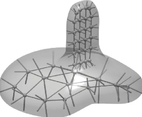
Figure 2.2: An object with two parts represented by a two-figure m-rep.

A multi-figure m-rep relieves the burden of the exact Blum condition for a branching axis by its geometric definition of connections between adjacent object parts and its replacement of the branching part of a Blum medial axis representing little volume by a skeletal structure [Damon (2005)], which is the underlying medial structure for a smooth transition between each pair of connected parts, to be detailed in section 4.2.3.

Overall, the relaxed branching structure in a multi-figure m-rep has the following advantages:

1. The interrelations and transformations between a pair of adjacent figures are ex-plicitly defined by the hinge geometry, which allows each one of the two medial figures to deform with or without affecting the other;

2. A subtractive part as an indentation subfigure connects in a completely equivalent way as an additive part as a protrusion subfigure to its host figure, shown in figure 2.2. This significantly simplifies the statistical analysis on objects with indentations or protrusions;

(44)

4. The fact that a host figure stands for the majority of an object volume and is visited before its subfigure in a multi-scale fitting or segmentation process provides more stability.

Given a medial shape representation, we often need to calculate its implied bound-ary. In the cm-reps of Yushkevich and Terriberry, different approximation schemes are applied directly to their shape primitives, i.e., medial control points, and the approx-imation schemes are strictly constrained by the Blum condition. In the cm-reps, no implied boundary points can be calculated, not even for the medial control points, until smooth approximations are derived from the control points for both the medial sheet and the radial field because a cm-rep implied boundary solely depends on the underly-ing spokes, and the underlyunderly-ing spokes can only be calculated from the derivatives of the medial sheet and radius field. It is different for a discrete m-rep because the included spokes in an m-rep imply a coarse boundary mesh connecting all the spoke ends. As a result, there are two types of methods to calculate an m-rep implied boundary by an interpolation either on the mesh of medial atom spoke ends or directly on medial atoms to form an interpolated medial sheet and spoke field.

The method based on the Catmull-Clark subdivision [Thall (2004)] was the first one proposed to generate the implied boundary of an m-rep. This method uses an interpolating variation of the Catmull-Clark subdivision scheme and belongs to the first type of interpolation methods on m-reps. This interpolation method is applied to the surface points and approximate normals implied by medial atoms in an m-rep figure: medial spoke end points as the surface points and spoke directions as the surface normals at those surface points.

A new method will be proposed in this dissertation to construct the boundary from an m-rep, by a constrained medialatom interpolation, which directly interpolates m-rep atoms and belongs to the second type of interpolation methods on m-reps.

(45)

computation. However, the new method based on atom interpolation has the advantage of generating a spoke field on a medial sheet, which allows us to apply constraints to enforce a shape model to stay proper (legal) or to implement medially based integrations on the interpolated medial spoke field to assist deformable model fitting or image seg-mentation. Furthermore, the new method provides a full parameterization of the entire object volume by the interpolated spokes. The atom interpolation will be described in detail by chapter 3.

I have reviewed three series of medial shape representations. The main advantages of them are as follows.

1. They are volumetric representations: they model not only the boundary but also the interior of an object and the immediately adjacent exterior of the object. This provides robust accesses to volumetric image intensities.

2. They are multiscale representations: they can represent the geometry of objects or object complexes in a coarse-to-fine fashion. Multiscale approaches for deformable models have proven to be more robust to image defects such as noise, aliasing, and missing data. Also, multiscale methods are more robust to the local opti-mum problem during the maxiopti-mum a posterior (MAP) optimization for image segmentation;

3. They provide a figural coordinate system: such a coordinate system can be used to describe the local interrelationships among adjacent object parts or adjacent objects in an object complex.

(46)

2.3 Mathematics of a Medial Structure

This section reviews the radial shape operator and itsrSrad matrix, and the edge shape

operator and itsrSE matrix. These algebraic operators characterize the geometry behind

a medial structure. The rest of this section lays out the definition and calculation of both the shape operators and their extensions on a Blum medial structure, the application of these shape operators to any smooth spoke field attached to a smooth medial sheet, called a skeletal structure [Damon (2005)], and two legality conditions based on the geometric property of these shape operators.

Recall that a shape operator defined on a 3D surface describes how the surface normal swings along the surface, i.e., how a surface curves locally. Analogously, aradial shape operator Srad tells how a unit length medial spoke U changes while walking on

the interior of a medial sheet, and an edge shape operator SE tells how U changes

while walking along the edge curve of a medial sheet. Both the radial shape operator and the edge shape operator are defined by Damon in [Damon (2003, 2004, 2005)]. These medial shape operators record derivative information of a medial sheet surface and medial spokes attached to it. A radial shape operator and an edge shape operator can also be extended to an rSrad matrix and an rSE matrix, respectively, to represent

the rate of change of full spokes S instead of unit length spokes. Next I will show how to calculate the shape operators and their extended matrices, starting with the radial shape operator and the rSrad matrix followed by the edge shape operator and the rSE

matrix.

Each internal medial point on the medial sheet has a spoke at each side of a medial sheet; thus the spoke fields on a medial sheet are double-valued. So there are two radial shape operators defined for each medial atom: one for each spoke at one side of the medial sheet. The following description focuses on one radial shape operator because the same description applies to the other radial shape operator of an m-rep atom.

(47)

field S(u) with unit length spoke direction U(u) and spoke length r(u) on the side of the continuous medial sheet p(u). S(u) = r(u)·U(u), and u = (v1, v2) parameterizes the two dimensional medial sheet and spoke field. The derivatives of the unit length spoke directionU(u) by (v1, v2) are calculated as follows, withUand pv1/v2 being 1×3

row vectors.

∂U

∂vi

=a0,iU−ai,1pv1 −ai,2pv2, where i= 1,2, (2.6)

or rewritten in matrix form:

∂U

∂u =



 

a0,1

a0,2





U−



 

a1,1 a1,2

a2,1 a2,2

     

p_v₁ p_v₂





 (2.7)

where ∂_∂U_u is a 2×3 matrix with row i as the vector ∂_∂vU

i, and where pv1 and pv2 are

the derivatives of the medial sheet p by parameters v1 and v2. In these equations, the derivative ofUis decomposed by a generally non-orthogonal projection along the spoke direction U to the tangent plane of the medial sheet spanned byp_v₁ and p_v₂.

Let Au =



 

a0,1

a0,2





, and let Srad = 

 

a1,1 a2,1

a1,2 a2,2





. Srad is called the radial shape

operator. In general, the radial shape operator has the following properties:

• 2×2 matrix

• not self-adjoint

Then (2.17) implies

∂U

∂u =AuU−S

T rad



 

p_v₁ p_v₂





, (2.8)

U(u) is of unit length, implyingU·UT = 1 and ∂_∂U_u ·UT =

(48)

Au =STrad



 

p_v₁ p_v₂





U

T _(2.9)

Substituting (2.9) into (2.17) yields the means of computing Srad given ∂_∂U_u, U and



 

p_v₁ p_v₂



 :

Srad =

∂U

∂u ·Q

−1

T

(2.10)

where Q=



 

p_v₁ p_v₂





(U

T

U−I) is a 2×3 matrix.

That is to say, Srad depends on the spoke directionU, and the derivatives of Uand

p.

Besides the radial shape operator Srad describing the rate of change of unit length

spokes, we also need to describe the rate of change of full spokesS=rU. The derivative of a full spoke S=rUof length r is given as follows, based on the derivative of a unit length spoke U.

∂S

∂u =

∂(rU)

∂u =r

∂U

∂u +



 

rv1 rv2





U (2.11)

Substituting (2.17) and (2.9) into (2.11) yields

∂S

∂u =rS

T rad



 

p_v₁ p_v₂





(U

T_U₋_{I) +}



 

rv1 rv2





U (2.12)

(49)

rSrad =       ∂S

∂u +



 

p_v₁UT p_v₂UT

  U   Q T

(QQT)−1



 

T

(2.13)

Based on the compatibility condition, equation (2.13) shows how to compute an

rSrad matrix given the derivatives of S, p, and U in a Blum medial axis. However in

a general skeletal structure [Damon (2004, 2005)], in which spokes are not necessarily perpendicular to the object boundary, the derivatives of r are not directly related to the derivatives of the medial sheet pand have to be calculated directly instead of being implied by the compatibility condition. In the case of a skeletal structure, the calculation of rSrad is shown in equation (2.14):

rSrad =

      ∂S

∂u −



 

rv1 rv2

  U   Q T

(QQT)−1



 

T

(2.14)

Besides the regular spokes on both sides of a medial sheet, there are also end spokes lying on the edge curve of the medial sheet. As a result, each end m-rep atom has an extra bisector spoke corresponding to the boundary crest. This bisector spoke swings along the edge curve of the medial sheet, so a different shape operator is needed to record its rate of change while walking along the edge curve. An edge shape operatorSE serves

this purpose. The following describes the calculation of an edge shape operator and its extension rSE matrix.

Let δ(t) be the edge curve of a medial sheet, parameterized by t, let p₀ be an edge point on δt as an edge medial point of interest, and let p(v1, v2) be a local edge parameterization of an open set W with p(0,0) = p₀ ∈ δ(t) (the exact definition of this local edge parameterization is out of the scope of this dissertation, and detail of this special parameterization can be found in [Damon (2005)]). Assume that p(v1, v2) is chosen such that the derivative of p along v1 is aligned with the tangent direction of

δ(t) atp₀, i.e.,p0_v

(50)

edge parameterization to cUtan, for cUtan the tangential component of U and c ≥ 0.

SE is then calculated by projecting the derivative ofUvia a non-orthogonal projection

along Uto a plane, spanned by n, the normal to the medial sheet at p₀, and p_v₁:

∂U

∂vi

=a0,iU−ai,1pv1 −ai,2n, wherei= 1,2, (2.15)

or rewritten in matrix form:

∂U

∂u =



 

a0,1

a0,2





U−



 

a1,1 a1,2

a2,1 a2,2

     

p_v₁ n





 (2.16)

where ∂_∂U_u, p_v₁, and p_v₂ are defined as in .

SE =



 

a1,1 a2,1

a1,2 a2,2





is defined as the edge shape operator. In general, the edge shape

operator also has the following properties:

• 2×2 matrix

• not self-adjoint

Let Au,E =



 

a0,1

a0,2





. Then (2.16) implies

∂U

∂u =Au,EU−S

T E



 

p_v₁ n





, (2.17)

Following the derivation of the Srad and its extensionrSrad, the means of computing

SE and its extension rSE given ∂_∂U_u, Uand



 

p_v₁ n





are as follows:

SE =

∂U

∂u ·Q

−1

E

T

(2.18)

where Q_E =



 

p_v₁ n





(U

(51)

rSE =       ∂S

∂u +



 

p_v₁UT p_v₂UT

  U   Q T

E(QEQ T E)−1



 

T

(2.19)

which is based on the compatibility condition in a Blum medial axis.

rSE =

      ∂S

∂u −



 

rv1 rn   U   Q T

E(QEQ T E)−1



 

T

(2.20)

which is not enforcing the compatibility condition for a general skeletal structure. Equations (2.14) and (2.20) show the full power of anrSradmatrix and anrSE matrix

lying in the fact that they are applicable to a skeletal structure, i.e., any smooth spoke field on a smooth medial sheet surface, either one-sided or two-sided. A Blum medial axis is a special case of a two-sided skeletal structure such that each medial axis point implies a maximal sphere inside the object and tangential to the object boundary at two or more points, i.e., the medial spokes implied by a Blum medial axis are perpendicular to the implied boundary at the spoke end points. The rSrad and rSE matrices allow

us to work with a skeletal structure, which can be non-Blum, such as the interpolated spoke field of a blend region in a multi-figure m-rep, to be described in section 4.2.3.

So far this section has focused on the algebraic property of the two medial shape operators and their extensions, recording first order derivatives of a medial sheet and medial spokes. Both the shape operators and their extensions also have a geometric property that is crucial to two medial legality conditions, coming next.

(52)

interior of the medial sheet p and the corresponding spoke directions U, curves and swings locally, and the generalized eigenvalue of (SE,I1,1), computed as a2−,12 ·det(SE),

reflects how the edge curve and its attached end spokes of a medial axis change.

As an extension to a radial shape operator, an rSrad matrix automatically

incorpo-rates the curving of the interior of the medial sheet p when simultaneously measuring the rate of change of the full spokesSon the interior of the medial sheet; as an extension to an edge shape operator, anrSE matrix automatically incorporates the curving of the

edge curve of the medial sheet p when simultaneously measuring the rate of change of the full spokesSalong the medial sheet edge curve. The eigenvalues of anrSrad matrix,

i.e., theradial principal curvatures, and the generalized eigenvalue of anrSE matrix, i.e.,

the principal edge curvature will be used in the two legality conditions to be described next [Damon (2005)].

Consider a local radial flow from the interior of a medial sheetpalong one of the two spokesS+1,−1to the implied boundary asϕ(p, t) =p+tS, t∈[0,1]. ϕcan be generalized to a global radial flow from the medial sheet to the entire object boundary via the doubled-sided spoke field on the medial sheet. The spoke field is legal if and only if the Jacobian matrix of this global radial flowϕis never singular. This implies that for a legal spoke field in the interior of a medial sheet, i.e., one free of any intersections among the spokes, it has to fulfill a legality condition called the radial curvature condition [Damon (2005)] shown below. The radial curvature condition is mathematically equivalent to the constraints in the Blum condition (listed at the end of section 2.2.1).

λri <1, where λri =rκri, for all positive real eigenvalues λri, i= 1or2 of rSrad.

(2.21) where r is the interior spoke length.