NON-RIGID BODY MECHANICAL PROPERTY RECOVERY FROM IMAGES AND VIDEOS
Shan Yang
A dissertation submitted to the faculty of the University of North Carolina at Chapel Hill in partial fulfillment of the requirements for the degree of Doctor of Philosophy in the Department of
Computer Science.
Chapel Hill 2018
©2018 Shan Yang
ABSTRACT
Shan Yang: Non-rigid Body Mechanical Property Recovery from Images and Videos (Under the direction of Ming C. Lin)
Material property has great importance in surgical simulation and virtual reality. The mechanical properties of the human soft tissue are critical to characterize the tissue deformation of each patient. Studies have shown that the tissue stiffness described by the tissue properties may indicate abnormal pathological process. The (recovered) elasticity parameters can assist surgeons to perform better pre-op surgical planning and enable medical robots to carry out personalized surgical procedures. Traditional elasticity parameters estimation methods rely largely on known external forces measured by special devices and strain field estimated by landmarks on the deformable bodies. Or they are limited to mechanical property estimation for quasi-static deformation. For virtual reality applications such as virtual try-on, garment material capturing is of equal significance as the geometry reconstruction.
The classifier achieves up to91%for predicting cancer T-Stage and 88%for predicting Gleason score. To recover the mechanical properties of soft bodies from a video, I propose a method which couples statistical graphical model with FEM simulation. Using this method, I can recover the material properties of a soft ball from a high-speed camera video that captures the motion of the ball.
ACKNOWLEDGEMENTS
The five years’ Ph.D life has been an incredible experience for me. First and foremost, I would like to thank my advisor Prof. Ming C. Lin for taking me as her Ph.D student in the first place. She has been so kind to guide, help and support me through this journey. I would also love to thank my Ph.D committee members: Prof. Dinesh Manocha for all the advice on my papers; Prof. Vladmir Jojic for opening the gate of machine learning to me; Prof. Tamara Berg for all the suggestions on my garment recovery paper; Prof. Chris Bregler for all the great ideas and support through my internship.
It is not possible to finish this journey without all the kind help and support from my all of my friends especially Licheng Yu and all the gamma members.
TABLE OF CONTENTS
LIST OF TABLES . . . xii
LIST OF FIGURES . . . xiv
LIST OF ABBREVIATIONS . . . xxi
LIST OF SYMBOLS . . . xxii
1 Introduction . . . 1
1.1 Cloth Material Property Recovery . . . 5
1.2 Thesis Statement . . . 6
1.3 Main Results . . . 7
1.3.1 Image-based Multi-region Deformable Body Material Recovery . . . 7
1.3.2 Video-based Deformable Body Material Recovery . . . 7
1.3.3 Classification of Prostate Cancer Grades and T-Stages based on Tissue Elasticity . . . 8
1.3.4 Single-view Image-based 3D Garment Reconstruction . . . 8
1.3.5 Learning-based Cloth Material Recovery from A Video . . . 9
1.4 Organization . . . 9
2 Previous Work . . . 11
2.1 Deformable Body Simulation . . . 11
2.2 Human-Tissue Mechanical Property Recovery . . . 12
2.2.1 Measurement-based Methods . . . 15
2.2.2 Elastography . . . 15
2.2.4 Probabilistic Graphical Models . . . 16
2.3 Cloth Mechanical Property Recovery . . . 17
3 Multi-region Image-based Elasticity Recovery . . . 18
3.1 Introduction . . . 18
3.2 Method . . . 19
3.2.1 Geometry Reconstruction and Mesh Generation . . . 19
3.2.2 Quasi-Static Process Elasticity Parameter Estimation . . . 20
3.2.2.1 Forward Simulation . . . 21
3.2.2.2 Material Model . . . 22
3.2.2.3 The Boundary Condition . . . 24
3.2.2.4 Distance-Based Objective Function . . . 25
3.2.2.5 Multi-Region Elasticity Parameter Estimation . . . 26
3.2.2.6 The Inverse Step . . . 28
3.2.3 Sensitivity Analysis . . . 33
3.3 Experiments . . . 37
3.3.1 Multi-Region Elasticity-Parameter Reconstruction . . . 37
3.3.2 Correlating Estimated Tissue Parameters with Cancer T-Stages . . . 39
3.3.3 Performance Analysis for Quasi-Static Parameter Estimation . . . 41
3.3.4 Applications . . . 42
3.3.5 Comparison with Other Approaches . . . 44
3.4 Conclusion and Future Work . . . 45
4 Video-based Soft-body Mechanical Property Recovery . . . 46
4.1 Introduction . . . 46
4.2 Method . . . 47
4.2.1 Generalized Dynamic Process and Decoupled State Parameter Estimation . . 47
4.2.3 Bayesian Parameter Estimation . . . 49
4.2.4 Unscented Kalman Filter for Parameter Estimation . . . 50
4.2.5 Coupled State Estimation . . . 53
4.3 Experiments . . . 53
4.3.1 Synthetic Heart Experiment . . . 55
4.3.2 Mechanical Parameters Recovered from Videos . . . 57
4.4 Conclusion and Future Work . . . 59
5 Classification of Prostate Cancer Grades and T-Stages based on Tissue Elasticity Using Medical Image Analysis . . . 61
5.1 Introduction . . . 61
5.2 Method . . . 62
5.2.1 Forward Simulation: BioTissue Modeling . . . 63
5.2.2 Inverse Process: Optimization for Parameter Identification . . . 64
5.2.3 Classification Methods . . . 65
5.3 Results. . . 65
5.3.1 Preprocessing and Patient Dataset . . . 65
5.3.2 Cancer Grading/Staging Classification based on Prostate Elasticity Parameters 66 5.4 Conclusion . . . 68
6 Single-view Image-based Garment Recovery . . . 70
6.1 Introduction . . . 70
6.2 Related Work . . . 72
6.3 Method . . . 75
6.4 Data Preparation . . . 76
6.4.1 Data Representations . . . 76
6.4.2 Preprocessing . . . 78
6.4.3 Initial Garment Registration . . . 79
6.5.1 Overview . . . 81
6.5.2 Garment Types, Patterns, and Parameters . . . 82
6.5.3 From Wrinkle Density to Material Property and Sizing Parameters . . . 83
6.5.4 Optimization-based Parameter Estimation . . . 85
6.6 Joint Material-Pose Optimization . . . 87
6.6.1 Optimal Parameter Selection . . . 87
6.6.2 Application to Image-Based Virtual Try-On . . . 88
6.7 Results and Discussion . . . 89
6.7.1 Garment Recovery Results . . . 89
6.7.2 Comparison with Other Related Work . . . 93
6.7.3 Performance . . . 95
6.7.4 Discussions and Limitations . . . 95
6.8 Conclusion and Future Work . . . 97
7 Learning-based Cloth Material Recovery from Video . . . 98
7.1 Introduction . . . 98
7.2 Related Work . . . 100
7.3 Method . . . 102
7.4 Visual, Material and Motion Representation . . . 102
7.4.1 Appearance Representation . . . 102
7.4.2 Material Representation . . . 103
7.4.2.1 Material Model . . . 103
7.4.2.2 Parameter Space Discretization . . . 104
7.4.3 Motion Sub-space . . . 105
7.5 Learning Method . . . 106
7.5.1 Deep Neural Network Structure . . . 106
7.6.1 Data Generation . . . 109
7.7 Experiments . . . 110
7.7.1 Data Preparation . . . 111
7.7.2 Results . . . 111
7.7.2.1 Baseline Results . . . 111
7.7.2.2 Validation of My Method . . . 112
7.7.2.3 Comparison . . . 113
7.7.3 Application . . . 114
7.7.4 Discussion and Limitations . . . 114
7.8 Conclusion and Future Work . . . 115
8 Conclusion . . . 116
8.1 Summary of Results . . . 116
8.1.1 Image-based Multi-region Deformable Body Material Recovery . . . 116
8.1.2 Video-based Deformable Body Material Recovery . . . 117
8.1.3 Classification of Prostate Cancer Grades and T-Stages based on Tissue Elasticity . . . 118
8.1.4 Single-view Image-based 3D Garment Reconstruction . . . 119
8.1.5 Learning-based Cloth Material Recovery from A Video . . . 120
8.2 Limitations. . . 120
8.3 Future Work . . . 122
LIST OF TABLES
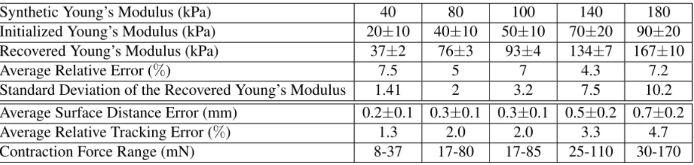
3.1 Multi-Region Elasticity Parameter Reconstruction . . . 38 3.2 Multi-Region Elasticity Parameter Reconstruction . . . 39 3.3 T-stages for prostate cancer definition . . . 41 4.1 The result for the synthetic heart experiment with noises in the
initializa-tion. The relative error of the recovered Young’s modulus is within7.5%of the ground-truth values. Our method reduces the average surface-tracking error
down to less than5%. . . 56 4.2 Impact of initial velocities on recovered Young’s moduli. . . 59 4.3 Comparison with results of (Wang et al., 2015) and experimental
mea-surements. The measured Young’s modulus for the tennis ball is taken from (Sissler et al., 2010; W´ojcicki et al., 2011) and for the foam ball is derived from (Moore et al., 2007). The recovered Young’s modulus using our method is within the range of the Young’s modulus measured, the Young’s
modulus recovered using (Wang et al., 2015) is not. . . 60 6.1 The accuracy of the recovered sizing and material parameters. The
accu-racy of the recovered sizing and material parameters of the t-shirt and the pants
(in percentages). . . 92 6.2 The accuracy of recovered garment curvature and material parameters.
The accuracy of the recovered garment local mean curvature and material
parameters of the skirt (in percentages). . . 92 6.3 Difference between the recovered human body joint angles and the
ground-truth values (in Degree) for different poses shown in Fig. 6.11.
. . . 93 7.1 Material parameter sub-space validation. The floating point numbers
show the estimated stretching/bending parameter coefficients(˜p,˜k), while the numbers in the parenthesis are the corresponding stretching/bending parameter
(p, k)in my defined subspaceP. . . 107 7.2 Testing results. The models are trained with the arm bending motion and wind
blowing motion. Then they are tested on 432 simulated arm bending/wind blowing videos, where the ground truth is known. My method achieved up to71.8%of accuracy for predicting 54 classes of materials for arm bending
7.3 Stiffness/density correlation r values for (Bouman et al., 2013) vs. Ours My method outperforms both (Bouman et al., 2013) and human perception, achieving the highest correlation value of0.77and0.84respectively for
LIST OF FIGURES
1.1 Examples of soft bodies in movies. (a) The long and curvy hair of Merida in the movie Brave. (b) The strong muscles of both Maui and Moana in the
movie Moana. (c) The gorgeous dresses of Queen Elsa and Anna in the movie Frozen. . 1 1.2 Example of the virtual try-on system with MagicMirror®. . . 2 1.3 Surgeons prepare surgery with the da Vinci® surgical system. . . . . 4 1.4 Prostate cancer statistics (Cook, 2017). . . 5 1.5 Skirts with different material types (stylewe, 2014). Skirts with different
material properties showcase different appearances. . . 5 3.1 The Flow Chart of My Framework. My framework takes (at least) two sets
of images (medical images or other multi-view images) as input; I use these images to reconstruct 3D meshes. The initial guess at the elasticity parameter is based on standard values and is given prior to the start of the optimization process. For each optimization iteration, the body deformation is recomputed using FEM simulation. The value of the distance objective function is also re-evaluated. At the end of each iteration, the elasticity parameter is updated; the new, refined value is used by the finite element model to continue the
simulated-based optimization process. . . 19 3.2 The CT Image of Male Pelvic Area. The red dotted lines are the boundary
of my model reconstruction. . . 25 3.3 Reconstructed Contact Force of One Patient’s Prostate. The light colored
transparent surface is the reference mesh; the nontransparent surface is the
initial surface. . . 26 3.4 The Prostatic Urethra. The prostatic urethra naturally divides the prostate
into two parts. © Wikipedia(Gray, 1918) . . . 27 3.5 The 2D and 3D Illustration of the Nodes of Regions. (a) These nodes do
not contribute to the convergence of the optimization. (b) The figure on the left shows nodes shared by the two regions; the figure on the right shows the
3.7 The Sensitivity Analysis Results. (a) shows the relation between amount of deformation represented by the inner sphere’s radius changes vs. the relative elasticity parameter. (b) shows the relation between the change in deforma-tion per change in the relative elasticity parameter vs. the relative elasticity
parameter. . . 36 3.8 Different Regions of the Organ. left with a tumor embedded; right with
normal tissue. . . 38 3.9 Particle-Swarm Optimization Process: The blue dots are the particles and
the red dot signifies the ground truth. . . 39 3.10 The Relative Error vs. Tumor-to-Region Ratio. This figure shows the
relative error of elasticity parameters for the normal region recovered using
models with varying mesh resolutions plotted against the tumor-to-region ratio. . . 40 3.11 The Recovered Elasticity Parameter vs. Tumor-to-Region Ratio. This
figure shows the recovered elasticity parameter for the tumor region using
models with different mesh resolutions vs. the tumor-to-region ratio. . . 41 3.12 Box Plot of Estimated Average Elasticity Parameters. The estimated
elas-ticity parametersµ¯ of the prostate of the ten patients vs. their cancer stages
shows positive correlation. . . 42 3.13 The Running Time of the Reconstruction Process vs. the Number of
Threads Used. The running time decreases almost linearly with the increase
of the number of thread. . . 42 3.14 The virtual surgery application.(a) shows the liver, with elasticity parameter
reconstructed from patient data, resting on a plate. (b) is the screenshot of our virtual surgery system, using elasticity parameters for the prostate that were
reconstructed from patient data. . . 43 3.15 Animation from 2D Sketches. The three images in the first row are the
2D Sketches of three keyframes; the three images in the second row are the
simulation result of the corresponding keyframes. . . 43 4.1 The Flow Chart of Our Framework. Our framework takes a temporal
sequence of deformation samples as the input. The UKF takes in the observa-tions and drives the finite element simulation by optimizing both the hidden
parameter and hidden states. . . 48 4.2 The human heart anatomy. In this project I model the left and right
4.3 Reconstructed left ventricle and right ventricle of human heart. (a)-(b) the slices of a human heart ultrasound image © CETUS 2014 (Bernard et al., 2014), (c) the surface mesh of the reconstructed model, (d) the sliced view of
the tetrahedra mesh from the surface mesh in (b). . . 56 4.4 The computed contraction force and synthetic heart simulation result. (a)
the visualization of the contraction force on the surface of the 3D heart model using cool to hot color map, (b) the sliced view of the contraction force. (c) the simulated heart model by the end of systole phase, (d) the simulated heart
model by the end of diastole phase. . . 57 4.5 The convergence graphs for synthetic heart experiment.(a) shows our
framework reduces the distance between the surface with the optimized ma-terial parameter and the reference surface, as the framework iterates with the initial distance error at 3.2mm, (b) shows the convergence of the Young’s
modulus to the ground truth. . . 57 4.6 Input tennis video clips and the tracked surface mesh. (a)-(e) the clips of
the tennis video © Trevor Shannon (Shannon, 2009); (f)-(j) the tracked surface
mesh at the corresponding time stamp. . . 58 4.7 Input foam ball video clips and the tracked surface mesh. (a)-(e) the clips
of the tennis video © Trevor Shannon (Shannon, 2009); (f)-(j) the tracked
surface mesh at the corresponding time stamp. . . 59 5.1 Real Patient CT Image and Reconstructed Organ Surfaces. (a) shows one
slice of the parient CT images with the bladder, prostate and rectum segmented.
(b) shows the reconstructed organ surfaces. . . 66 5.2 Error Distribution of Cancer Grading/Staging Classification for
Per-Image Study. (a) shows error distribution of our cancer staging classification using the recovered prostate elasticity parameter and the patient’s age. For our patient dataset, the multinomial classifier (shown in royal blue and sky blue) outperforms the ordinal classifier (shown in crimson and coral). I achieve up to 91% accuracy using multinomial logistic regression and 89% using ordinal logistic regression for classifying cancer T-Stage based on recovered elasticity parameter and age. (b) shows the correlation between the recovered relative elasticity parameter and the Gleason score with/without the patient’s age. I achieve up to88%accuracy using multinomial logistic regression and
81%using ordinal logistic regression for classifying Gleason score based on
5.3 Error Distribution of Cancer Aggression/Staging Classification for Per-Patient Study. (a) shows the accuracy and error distribution of our recovered prostate elasticity parameter and cancer T-Stage. For our patient dataset, the multinomial classifier (shown in royal blue and sky blue) outperforms the ordinal classifier (shown in crimson and coral). I achieve up to84%accuracy using multinomial logistic regression and82%using ordinal logistic regression for classifying cancer T-Stage based on our recovered elasticity parameter and patient age information. (b) shows the correlation between the recovered relative elasticity parameter and the Gleason score. I achieve up to 77% accuracy using multinomial logistic regression and70%using ordinal logistic regression for classifying Gleason score based on our recovered elasticity
parameter and patient age information. . . 69 6.1 Garment recovery and re-purposing results. From left to right, I show an
example of (a) the original image(Saaclothes, 2015) ©, (b) the recovered dress and body shape from a single-view image, and (c)-(e) the recovered garment
on another body of different poses and shapes/sizes(Hillsweddingdress, 2015) ©. . . 70 6.2 The flowchart of my algorithm. I take a single-view image (ModCloth,
2015) ©, a human-body dataset, and a garment-template database as input. I preprocess the input data by performing garment parsing, sizing and features estimation, and human-body reconstruction. Next, I recover an estimated garment described by the set of garment parameters, including fabric material, design pattern parameters, sizing and wrinkle density, as well as the registered garment dressed on the reconstructed body. Finally, I perform joint material-pose optimization and show the recovered results using cloth simulation on the
virtual mannequin. . . 71 6.3 Template sewing pattern and parameter space of a skirt, pants, and
t-shirt. (a) The classic circle sewing pattern of a skirt. (b) My paramet-ric skirt template showing dashed lines for seams and the four parameters < l1, r1, r2, α >, in which parameter l1 is related to the waist girth and parameter r2 is related to the length of the skirt. (c) The classic pants sewing pattern. (d) My parametric pants template with seven parameters < w1, w2, w3, w4, h1, h2, h3 >. (e) The classic t-shirt sewing pattern. (f) My
parametric t-shirt template with six parameters< r, w1, w2, h1, h2, l1 >. . . 77 6.4 Initial garment registration process. (a) The human body mesh with the
skeleton joints shown as the red sphere and the skeleton of the arm shown as the cyan cylinder. (b) The initial t-shirt with the skeleton joint shown as the red sphere and the skeleton of the sleeve part of it shown as the cyan cylinder. (c) The t-shirt and the human body mesh are aligned by matching the joints.
6.5 Initial garment registration results. I fit garments to human bodies with
different body shapes and poses. . . 81 6.6 Material parameter identification results.(a) The local curvature estimation
before optimizing the bending stiffness coefficients (using the cool-to-hot color map). (b) The local curvature estimation after the optimization. (c) The original
garment image(ModCloth, 2015) ©. . . 83 6.7 Joint Material-Pose Optimization results. (a) The pants recovered prior to
the joint optimization. (b) The recovered pants after optimizing both the pose and the material properties. The wrinkles in the knee area better match with
those in the original image. (c) The original pants image(Anthropologie, 2015) ©. . . 87 6.8 Skirt and pants recovery results. I recover the partially occluded, folded
skirts from the single-view images in the first, fourth(ModCloth, 2015; AliEx-press, 2015) ©and seventh(Anthropologie, 2015) ©columns. The recovered human body meshes are shown in the second, fifth and eighth columns overlaid on the original images. The recovered skirts are shown in the third, sixth and
nineth columns. . . 89 6.9 Garment recovery results. For the first two rows, the input image (leftmost)
(ModCloth, 2015; AliExpress, 2015; RedBubble, 2015) ©and recovered gar-ment on the extracted human body. In the last row, the input image (leftmost)
and the recovered garment on a twisted body. . . 90 6.10 Image-based garment transfer results. I dress the woman in (a)
(Fashion-ableShoes, 2013; Boden, 2015) ©with the skirt I recovered from (b) (AliEx-press, 2015; ModCloth, 2015) ©. (c) I simulate my recovered skirt with some wind motion to animate the retargeted skirt, as shown in (d). Another example
of garment transfer is given in (e) - (h). . . 91 6.11 Synthetic evaluation scenes. (a)-(c) fixed body shape with different poses.
(d)-(e) fixed body shape with a skirt of different material. (f)-(j) same scene
setup as (a)-(e) but different lighting condition. . . 92 6.12 Comparison. (a) One frame of the video along with (b) the CMP-MVS results
before and (c) after smoothing. (d) My results using only one frame of the video. . . 94 6.13 Comparison.(a) One frame of the multi-view video along with (b) the
CMP-MVS results before and (c) after smoothing. (d) My results using only one
frame of the video. . . 94 6.14 Comparison. (a) input image (© 2015 ACM) from paper Chen et al. (Chen
et al., 2015) Figure 12. (b) my garment recover results from only a single-view RGB image (a). (c) recovery results (© 2015 ACM) from Chen et al. (Chen
6.15 Comparison. (a) input image (© 2015 Wiley) from Figure 3 in Jeong et al. (Jeong et al., 2015). (b) my garment recover results from (a). (c) recovery
results (© 2015 Wiley) from Jeong et al. (Jeong et al., 2015). . . 95 7.1 Learning-based cloth material prediction and material cloning results. (a)
learning samples generated using the state-of-art physically-based cloth sim-ulator Arcsim(Narain et al., 2012) (b) example real-life cloth motion videos presented in(Bouman et al., 2013) (c) simulated skirt with the material type predicted from the real-life video in (b) using the learned model from samples
presented in (a). . . 98 7.2 An overview of my method. My cloth material recovery method learns an
appearance-to-material mapping model from a set of synthetic training samples. With the learned mapping model, I perform material-type prediction given a
recorded video of cloth motion. . . 99 7.3 Stretching and bending parameters sensitivity analysis results. (best view
in color) The x-axis is the reciprocal of parameter ratios to the basis material. The y-axis is the maximum amount of deformation of the cloth, i.e., maximum amount of stretching or maximum curvature, respectively. I use the vertical lines with different colors to represent the 10 types of materials presented
in (Wang et al., 2011a). . . 106 7.4 Appearance-to-material learning method. I apply CNN and LSTM (the
original LRCN design presented in (Donahue et al., 2015a)) to learn the
mapping between appearance and material. . . 107 7.5 The five-layer CNN structure. The original design is presented
in (Krizhevsky et al., 2012) . . . 108 7.6 Learned CNN conv5-layer activation visualization. (best view in color) I
overlay the conv5 layer activation using the “jet” color map with the original image. The model is trained with my simulated data set with the cloth
wind-blowing motion. . . 108 7.7 Data generation pipeline. My simulated data learning samples generation
pipeline consists of two steps: cloth simulation and image rendering. . . 109 7.8 Simulated data showcase. The first three rows are example frames from my
Wind-blowing data set with the cloth in pose-1. The bottom two rows are example frames from my Wind-blowing simulated data set with the cloth in
7.9 Material cloning results. The first column are the input cloth motion videos(Bouman et al., 2013). I predict the material type of the cloth in these input videos and clone those material on to the skirt. The simulated skirt are
LIST OF ABBREVIATIONS
LIST OF SYMBOLS
C material property parameters of the garment G garment (sizing) parameters
Gpants < w1, w2, w3, w4, h1, h2, h3 > Gskirt < l1, r1, r2, α >
Gtop < r, w1, w2, h1, h2, l1 >
U 2D triangle mesh representing garment pattern
u vertex of the 2D garment pattern mesh
V 3D triangle surface mesh of the garment
V simulated 3D triangle surface mesh of the garment
Bbody skeleton of 3D human body mesh
Bgarment skeleton of 3D garment mesh
x vertex of the 3D triangle mesh
P average wrinkle density of the 2D segmented garment in the image
k bending stiffness parameters
w stretching stiffness parameters
F deformation gradient of the deforming garment K regional average curvature, 1D scalar
S 2D garment silhouette
Ψ bending energy of the garment Φ stretching energy of the garment
υij rigging weights of the 3D garment mesh
β joint angles of the skeleton of the 3D garment mesh
Dc garment database
CHAPTER 1: INTRODUCTION
From the soft tissue in our human body to the garments we wear everyday, deformable objects are ubiquitous. We interact with soft objects daily: when we comb our hair, dress ourselves with different styles of garments, and eat various types of delicious food. The physics, such as the mechanical properties of those deformable bodies, make them distinguishable via touch. This interaction with soft objects make us aware of their deformation behavior. Over time, we have been trained to develop this inner simulation system to predict the motion of those soft objects when we only have the visual of such items. For instance, we would expect a cotton-like textured t-shirt to be much softer than a linen-like textured cloth and curly hair to be more bouncy than straight hair.
For movies, animations and virtual reality applications, we prefer soft objects to be modeled accurately. For example, in the animations shown in Fig. 1.1, we would expect to see that Merida’s hair, Maui and Moana’s muscle and Queen Elsa and Anna’s dresses behave exactly the same way as our own hair, muscle and dresses. Movides are not the only example; real-world physics especially
Figure 1.1:Examples of soft bodies in movies.(a) The long and curvy hair of Merida in the movie Brave. (b) The strong muscles of both Maui and Moana in the movie Moana. (c) The gorgeous dresses of Queen Elsa and Anna in the movie Frozen.
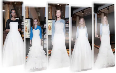
Figure 1.2:Example of the virtual try-on system with MagicMirror®.
world. In particular, the application of virtual try-on garment material properties changes both the appearance and the fit. Fig. 1.2 shows a virtual try-on system from MagicMirror®. This system helps brides easily try out wedding dresses. However, a simple 3D garment overlaying our body is far from sufficient for a multimodal virtual try-on experience. Users will wish to change their pose to see how the garment fits. In order to provide such an experience, a physically-based simulation with the material properties of the garment as close as possible to real-world materials is crucial.
deformable bodies based on given hand drawings of keyframes. Automatic parameter identification from real-world data, such as simulation results, images, audio, video, and animators’ sketches, is thus becoming a topic of increasing interest in computer animation (Bickel et al., 2010; Wang et al., 2011b; Miguel et al., 2012a, 2013; Ren et al., 2013).
For example, the use of material-property estimation in the simulation of cloth has been suggested in (Wang et al., 2011b; Miguel et al., 2012a); it has also been used in procedures for designing and fabricating materials that produce a certain deformation behavior (Bickel et al., 2010). These parameter estimation methods focus on materials that can be taken into a specialized video capturing system to measure displacements, and (in the case of elasticity parameters) often require a force measuring device (Pai et al., 2001; Bickel et al., 2009).
Beyond virtual reality applications, non-rigid materials are widely used in medical robotics, design and manufacturing, virtual surgery for soft robot planning, procedural rehearsal and virtual reality applications etc. Medical robots (shown in Fig. 1.3) have the potential to perform surgical procedures beyond current clinical capabilities. Identification of mechanical properties, such as tissue elasticity parameters, is critical to enable medical robots to safely operate within highly unstructured, deformable human bodies and to compute desired, accurate force feedback for individualized haptic display characterized by patient-specific parameters for different tissues and organs. In addition to medical robots, simulations are also increasingly used for rapid prototyping of clinical devices, pre-operation planning of medical procedures, virtual training exercises for surgeons and supporting personnel, etc. And, bio-tissue elasticity properties are central to developing realistic and predictive simulation and for designing responsive, dexterous surgical manipulators. Furthermore, with increasing interest in 3D printing for rapid creation of soft robots consisting of flexible materials, the ability to easily acquire material properties from existing sensor data, such as medical images and videos, can help to replicate similar material properties.
Figure 1.3:Surgeons prepare surgery with the da Vinci®surgical system.
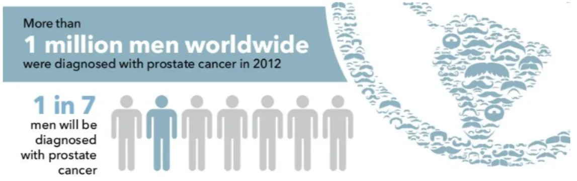
Figure 1.4:Prostate cancer statistics (Cook, 2017).
1.1 Cloth Material Property Recovery
Figure 1.5: Skirts with different material types (stylewe, 2014). Skirts with different material properties showcase different appearances.
often requires careful and lengthy design by a domain expert. The prior virtual try-on systems often use simple, fast image-based or texture-based techniques for a fixed number of avatar poses. Many of the virtual try-on systems assume either that the user selects one of a pre-defined set of avatars or that accurate measurements of their own bodies have been captured via 3D body scans.
More recent advances have been introduced in virtual try-on systems, such as triMirror and Avametric, that allow users to visualize what a garment might look like on them before purchasing. These methods enable 3D visualization of simulated garments, fast animation of dynamic cloth, and a quick preview of how the cloth drapes on avatars as they move around. To account for the effects of fabric materials under different conditions (e.g. varying poses, weight fluctuation, cloth-cloth interactions etc), a full cloth simulation is needed to predict how the fabric bends, wrinkles, or changes its physical appearance when the virtual human moves or changes his/her pose in various activities. One of the challenges that has not been addressed to date is to automatically determine and select the cloth material parameters required to simulate the garment fabric that visually exhibits the same physical behaviors, i.e. with the same simulated cloth material, as the one(s) shown in the given (online catalog) image of the garment on a fashion model. These simulation material parameters cannot always be obtained by physical measurements since they are often specific to a given computational model such as the one proposed by Wang et. al. (Wang et al., 2011a) of the simulated cloth. Generally they are acquired by tedious, time-consuming, and laborious manual tuning of multiple simulation parameters that result in the similar visual appearance as the real garment.
1.2 Thesis Statement
My thesis is as follows,
Material properties of the non-rigid objects presented in images or videos can be estimated
using a coupled deterministic simulation optimization, a stochastic statistical inferring based
To support this thesis statement, I present four methods: two methods couple physically-based deformable body simulation and optimization, one method applies machine learning for cloth material recovery from a video, and one statistically inferencing method.
1.3 Main Results
1.3.1 Image-based Multi-region Deformable Body Material Recovery
Material property of human tissue has great importance in medical applications. The recovered elasticity parameters can assist doctors with disease diagnosis and surgeons to perform better pre-op surgical planning. Previous non-invasive elasticity parameters estimation methods are limited to recover only one elasticity parameter of one deformable body at a time. The elasticity parameters of multiple resgions of a soft body such as a human organ can help doctors to further locate the cancerous area. To recover the material properties of multiple regions of a deformable body directly from an image, in Chapter 3 I propose to couple physically-based soft body simulation with Particle Swarm Optimization. The main contributions of my work are:
• A coupled physically-based soft body simulation with Particle Swarm Optimization;
• A multi-region image-based material recovery method.
1.3.2 Video-based Deformable Body Material Recovery
• An alternative approach to dynamically track the surface of a deformable body in motion; • Reconstruction of non-rigid mechanical properties from temporal sequences of deformation
samples using a probabilistic, graphical model.
1.3.3 Classification of Prostate Cancer Grades and T-Stages based on Tissue Elasticity
To study the possible use of tissue elasticity to help evaluate the prognosis of prostate cancer patients given at least two set of CT images, in Chapter 5 I analyze 29 prostate cancer patients data. I apply and improved the method proposed in Chapter 3 to estimate the individualized, relative tissue elasticity parameters directly from medical images. Using the recovered elasticity parameters, I train a multiclass classifier to predict the T-stage and Gleason scores of prostate cancer patients. The main contributions of my work are:
• An improved method that uses geometric and physical constraints to deduce the relative tissue elasticity parameters;
• Multiclass classification system for classifying T-stage and Gleason scores for prostate cancer patients;
• Demonstrate the feasibility of a statistically-based multiclass classifier as additional clinical aids for the physicians and patients to make more informed decision.
1.3.4 Single-view Image-based 3D Garment Reconstruction
garment fabric that visually exhibits the same physical behaviors. In Chapter 6, I present a method that recovers the garment with both material and sizing parameters from a single-view image. The main contributions of my work are:
• An image-guided garment parameter selection method that makes the generation of virtual garments with diverse styles and sizes a simple and natural task;
• A joint material-pose optimization framework that can reconstruct both body and cloth models with material properties from a single image;
• Application for virtual try-on and character animation.
1.3.5 Learning-based Cloth Material Recovery from A Video
Image and video understanding enables better reconstruction of the physical world. Existing methods focus largely on geometry and visual appearance of the reconstructed scene. The physical properties of the objects in the environment can further provide a more realistic human-scene interaction. In Chapter 7, I present a method to recover the material properties of cloth from a video using a deep neural network. The main contributions of my work are:
• A deep neural network based parameter learning algorithm;
• Application of physically-based simulated data of cloth visual-to-material learning.
1.4 Organization
The subsequent chapters of this dissertation are organized as follows.
Chapter 2 surveys previous work that is related to the thesis work including: physically-based deformable body simulation methods, human-tissue material recovery methods and cloth mechanical property identification methods.
Chapter 4 presents the graphical model based dynamic deformable body mechanical property recovery from video.
Chapter 5 shows real-life patient data analysis. I first identify the material properties of the prostate of each patient using my proposed method introduced in Chapter 2. Then I build a classifier using two features: recovered prostate mechanical property and patients’ age. I demonstrate in this chapter the effectiveness of the recovered material properties for cancer identification.
Chapter 6 presents a method which reconstructs garments from a single-view image.
CHAPTER 2: PREVIOUS WORK
In this chapter, I survey the previous work related to my thesis work. In the following sections, I first survey physically-based soft-body simulation methods which are the basis of my research. Then, I introduce previous work on human-tissue mechanical property recovery methods and cloth mechanical property recovery methods. Finally, I survey previous work on a deep neural network which is related to my proposed learning-based cloth material recovery method.
2.1 Deformable Body Simulation
Finite element method (FEM) (Bathe, 2006) is one class of physically-based deformable body simulation methods. FEM was proposed in general as a numerical method to solve the underlying governing partical differentiate equation (PDE). It is frequently used for flesh/mus-cle simulation (Teran et al., 2003, 2005; Sifakis et al., 2006; Irving et al., 2007) and surgery simulation (Bro-Nielsen, 1996; Bro-Nielsen and Cotin, 1996; Miller, 1999; Berkley et al., 2004).
Simulation of cloth and garments as one special kind of deformable body has also been extensively studied in computer graphics (Ng and Grimsdale, 1996; House and Breen, 2000; Bridson et al., 2002; Govindaraju et al., 2007). Methods for cloth simulation can also be divided in to classes based on the underlying numerical methods: mass-spring system based cloth simulation (Vassilev et al., 2001) and FEM-based cloth simulation (Narain et al., 2012).
2.2 Human-Tissue Mechanical Property Recovery
Medical robots have the potential to perform surgical procedures beyond current clinical capabilities. To enable medical robots to safely operate within highly unstructured, deformable human bodies are needed for designing responsive and dexterous surgical manipulators. In addition, virtual surgical simulation has also been increasingly used for rapid prototyping of clinical devices, pre-operation planning of medical procedures, virtual training exercises for surgeons and medical personnel, etc. And, tissue elasticity properties are important parameters for developing accurate and predictive surgical simulation. Futhermore, to compute desired and accurate force feedback for a haptic display requires knowledge about the deformation of soft tissues and organs, which are characterized by patient-specific elastic parameters for different tissues and organs.
Studies(Fowlkes et al., 1995) (Garra et al., 1997) show that tissue elasticity parameters are important indicators of cancer and other diseases. Traditional cancer detection methods such as palpation have limitations. For tissues that locate inside the human body and far from the skin, procedures like palpation cannot reach. Besides, these methods are based on the empirical knowledge of the doctor. Further for each patient, the normal elastic properties may vary making it difficult for the doctor to establish a diagnoses standard. Thus, researchers proposed methods that are based on scientific computing instead of the sense of the doctor to estimate the elastic parameters of soft tissue. The emerging field of elastography tries to solve this problem. Methods that are based on medical image analysis and FEM based simulation provide a rigorous way of calculating the elasticity parameters of the potential cancer tissues.
Estimation of material parameters for human tissues is also well-studied in medical image analysis, where it is used in screening and detecting tumors, as cancerous tissues tend to be stiffer than healthy tissues. There are mainly two kinds of soft tissue elasticity properties estimation method (Samur et al., 2007): invasive and non-invasive techniques. The invasive methods rely on a device to measure the displacement and force response (Carter et al., 2001; Kauer et al., 2002a; Rosen et al., 1999). These methods take organ samples either out of the human or animal bodies and perform the experiment in-vitro (out side the body) or do the procedure in-situ (inside the body). The collected data are then used to solve the inverse problem, which is to recover the elasticity properties, by constructing a polynomial interpolation (Bicchi et al., 1996) or by using a finite element model (Gao et al., 2009; Misra et al., 2010; Samur et al., 2007).
two-dimensional representations of the moving tissue. More sophisticated imaging techniques, such as magnetic resonance imaging (MRI)(Chenevert et al., 1998; Van Houten et al., 1999)and computed tomography (CT), produce three-dimensional images of the deforming tissues, allowing a more accurate measurement of displacement.
In the early days, ultrasound images were used in elastography(Krouskop et al., 1987). However, ultrasound images can only provide low resolution information. Compared to ultrasound images, magnetic resonance imaging (MRI) (Chenevert et al., 1998; Van Houten et al., 1999)and computed tomography (CT) images offer high resolution three-dimensional data. Based on magnetic resonance images or computed tomography images, three dimensional model can be reconstructed. Finite element method is used to simulate the deformation of the three dimensional model. By applying optimization method or other kinds of method, elasticity parameters are recovered.
2.2.1 Measurement-based Methods
Other than distance field based methods, there are also other measurement algorithms. The modality-independent elastography (MIE) method (Miga, 2002) measures the elasticity parameters by maximizing the image similarity based on a number of landmarks. However, this technique does not apply to all the soft tissues, as landmarks cannot always be found in some of the organs such as prostate. Statistical and machine learning algorithms have also been used to classify soft tissues and estimate the parameters using multi-spectral MR images (Liang et al., 1994).
2.2.2 Elastography
2D elastography (also known as elasticity reconstruction), can acquire ‘strain images’ or ‘elasticity images’ of soft tissues (Skovoroda and Emelianov, 1995; Rogowska et al., 2014; Bilston and Tan, 2015). Elastography is usually done by estimating the optimal deformation field that relates two ultrasound images, one taken at the rest state and the other taken when a known force is applied to the skin (Ophir et al., 1999; Rivaz et al., 2008). They were proposed to avoid the explicit measurement of the displacement. Van Houten et al. (Van Houten et al., 1999, 2001) used elastography methods to estimate the Young’s modulus distribution of a deformable body. These methods need high-resolution displacement fields to recover the elasticity parameter (Manduca et al., 2001). The displacement field can be obtained through an external device using a vibration actuation mechanism. External device is still required for both the force exertion on the soft tissue and the external force measurement. Special vibrator were placed inside the organ (Chopra et al., 2009) to complete the procedure. Other than distance-field-based methods for high-resolution magnetic resonance medical images, other video based method measure the displacement field from the video (Syllebranque et al., 2007).
or by performing an iterative optimization to minimize the error in the deformation field (Kallel and Bertrand, 1996; Balocco et al., 2008; Schnur and Zabaras, 1992). One limitation for this class of methods is that they require a device both to measure the external force and to exert external force on the deformable bodies.
2.2.3 Inverse Finite Element Methods
Inverse finite element methods use the implicitly known or computed external force to recover the mechanical property. Lee et al. proposed a model to estimate the Young’s modulus based on low-resolution CT images and no external force is required to set the boundary condition (Lee et al., 2012a). The most recent work on identification of mechanical properties based on surface tracking (Wang et al., 2015) proposed a decoupled iterative tracking and parameter estimation framework. They applied a combined probabilistic physically-based method for surface tracking. Then, the tracked surfaces of the static state are the input to the parameter estimation framework. This approach does not require external force to be measured, but uses the gravity as the boundary condition. This class of methods avoid both the explicit measurement of external force and the displacement field. But the input references need to be in static state.
2.2.4 Probabilistic Graphical Models
2.3 Cloth Mechanical Property Recovery
CHAPTER 3: MULTI-REGION IMAGE-BASED ELASTICITY RECOVERY
3.1 Introduction
Being able to estimate the elasticity parameters of the patients tissue accurately can greatly help with the diagnoses. For prostate cancer diagnoses, doctors need to sample the tissue of the prostate in order to be certain about stage of the cancer and the kind of cancer. This procedure, however, is done without the prior knowledge of which region to sample. Thus, the tissue sample may offer misleading information. If I can learn before hand the elasticity of the two parts of the prostate, the sampling result may be able to provide valuable information. For problem like this, previous elastography methods have their limitations.
Toward realizing the concept of 3D physiological humans, I propose perhaps one of the first elasticity parameter estimation algorithm for multiple, heterogeneous deformable bodies simultaneously using medical images1. My approach is based on a multi-dimensional optimization method that iteratively performs deformable body simulation using a finite element method on reconstructed organ models with the continuously refined, estimated elasticity parameters. The geometric models of organs are reconstructed based on low-resolution CT images. My objective function measures the sum of the distance between the nodes of the organ surface. In contrast to elastography methods (Becker and Teschner, 2007a; Eskandari et al., 2011; Zhu et al., 2003b), the only information I need is the displacement of the nodes of the organ surface. I do not need every pixel-wise displacement vector, thus no extra procedures need to be performed on the patient. Two sets of (medical) images are sufficient to recover the elasticity parameters using my method. Therefore, my method can be widely applicable to different imaging technology. It can be used 1In this work, I usecomputed tomography (CT)images. But, the algorithm is also applicable to magnetic resonance
for animatino of soft bodies (see supplementary video) and possibly for cancer staging using only low-resolution CT images.
two$or$more$sets$of$images$
3D$Geometry$ Reconstruc5on$
from$Images$
Parameter$Es5ma5on$ Using$$
Coupled$Simula5on? Op5miza5on$ ini5al$guess$of$the$ elas5city$parameters$
Interac5ve$Applica5ons$ and$
Computer$Anima5on$
Figure 3.1: The Flow Chart of My Framework. My framework takes (at least) two sets of images (medical images or other multi-view images) as input; I use these images to reconstruct 3D meshes. The initial guess at the elasticity parameter is based on standard values and is given prior to the start of the optimization process. For each optimization iteration, the body deformation is recomputed using FEM simulation. The value of the distance objective function is also re-evaluated. At the end of each iteration, the elasticity parameter is updated; the new, refined value is used by the finite element model to continue the simulated-based optimization process.
3.2 Method
Given (at least) two sets of multi-view images of a deformable object, my framework can automatically estimate elasticity properties within multiple regions of this model.
Fig. 3.1 provides an overview of my system. I assume that (at least) two sets of multiple-view images are given, along with some initial guess at the elasticity parameters. First, I offer an overview of how my method uses the input images to produce the geometrical reconstructions that are then used in the elasticity-parameter reconstruction. Next, I describe each component of my system in more detail.
3.2.1 Geometry Reconstruction and Mesh Generation
Medical Imagesare usually taken when the organs are in a static or quasi-static state. There are several widely-used imaging technologies, such as X-ray radiography, magnetic resonance imaging (MRI), medical ultrasonography or ultrasound, elastography, tactile imaging, thermography, nuclear medicine functional imaging, computed tomography (CT) scanning or computerized axial tomography (CAT), etc. Each set of CT or CAT scans provides image “slices”, or the cross-sectional images of anatomy. Variants of MRI and ultrasound images can be used to reconstruct anatomical 3D geometry using public-domain libraries such as ITK-SNAP (Yushkevich et al., 2006b) or commercial systems such as AVS, 3D-Doctor, MxAnatomy, etc.
2D Drawings and Sketchescan be converted to 3D models using widely available commercial CAD and 3D modeling systems, such as Rhino, Autodesk LABS, Dassault Systems SolidWorks, etc.
Multi-view Images from Cameras/Camcorderand other imaging technologies have been used for 3D geometry reconstruction. Excellent surveys of methods of extracting 3D models from images can be found in (Moons et al., 2010; Yushkevich et al., 2006b; Snavely, 2008; Wu, 2013b). These methods include algorithms using images for which camera parameters are unknown, uncalibrated structure-from-motion methods, metric reconstruction from images with additional knowledge about images, etc.
FEM Mesh Generationis accomplished by first building the input surface meshes as described above. If medical images (e.g. CT, MRI, etc.) are used as input they require an additional step before mesh generation: segmenting using ITK-SNAP (Yushkevich et al., 2006b) into multiple regions. After mesh simplification and smoothing, the entire region of interest can be tetrahedralized using TetGen (Si, 2007).
3.2.2 Quasi-Static Process Elasticity Parameter Estimation
3.2.2.1 Forward Simulation
This step uses the elasticity parameters generated from the inverse optimization process to compute the amount of deformation that the body would undergo. I use the FEM to solve the following governing equation of the deformable body.
Z
Ω
δuTρ¨udΩ +
Z
Ω
δ(ε)Tσ dΩ−
Z
Ω
δuTbdΩ−
Z
Γ
δuTtdΓ = 0, (3.1)
withuas the displacement field,εas the strain tensor,σ as the stress tensor,bas the body force andtas the tractions on the boundaryΓof the deformable bodyΩ. For the quasi-static deformation process theu¨ =0. I can rewrite Eqn. 3.1 as
Z
Ω
δ(ε)Tσ dΩ−
Z
Ω
δuTbdΩ
−
Z
Γ
δuTtdΓ
= 0, (3.2)
with the first part of the equation as the internal body force and the second part as the external force. The computation of the stress force is determined by the material properties. Researchers have proposed many models for simulating different kinds of materials. These material models define the relation between the stress and the strain. To simulate the human organs in the abdomen and the soft tissue surrounding those organs, I use the isotropic hyperelastic material model, which is used commonly to approximate the deformation behavior of human tissue (Hu and Desai, 2004). The stress-strain relation for the hyperelastic material model is defined through the strain energy density functionΨ(energy per unit undeformed volume). I will be using the Green-Lagrange strain tensor
3.2.2.2 Material Model
The elastic behavior of deformable bodies varies for different materials. For small deformations, most elastic materials (e.g. springs) exhibit linear elasticity, which can be described as a linear function between stress and strain.
Linear Elasticity Material Model: The linearly elastic model assumes a constant variation of stress and strain according to Hooke’s law, with no permanent deformations after the applied stresses are removed. This holds true until the yield point, which is followed by an unrestricted plastic strain after yield. Assuming isotropic linear elasticity, I can write
σ =Dε, (3.3)
whereσis the stress tensor induced by thesurface forces,εis the strain tensor defined by the spatial derivatives of the displacementu, andDis a matrix defined by the material property parametersµ (D =D(µ)). Assuming an isotropic material, the commonly used material property parameters are Young’s modulusEand Poisson’s ratioν.
Isotropic Nonlinear Hyperelastic Material Model: For many materials, linear elastic mod-els cannot accurately capture the observed material behavior. Hyperelastic material modmod-els better describe the nonlinear material behavior exhibited when deformable bodies are subjected to large strains. For example, animal tissue and some common organic materials are known to be hypere-lastic (Hu and Desai, 2004). The nonlinearity is captured through the energy density functionΨ
for hyperelastic material models. The energy function is a function of the strain tensorεand the material property parametersµ, whereΨ=Ψ(ε,µ). With the energy function, the stress tensor is computed by taking the derivative of the energy function over the strain tensor.
σ = ∂Ψ(ε,µ)
∂ε (3.4)
Energy Function: The energy density function determines the nonlinear behavior of the deformable object. Human organs are hyperelastic and nearly isotropic. Generally speaking, for an isotropic material model, the energy function is expressed as a function of the invariantsI1,I2and
I3of the deformation gradientF,
I1 =λ21+λ 2 2+λ
2 3
I2 =λ21λ 2 2+λ
2 2λ
2 3+λ
2 1λ
2 3
I3 =λ21λ 2 2λ
2 3
(3.5)
and the deformation gradientFis a function of the strainF=F(ε). One general energy function for this class of incompressible materials, proposed by Rivlin (Rivlin, 1948), is
ΨR=
∞ X
i,j=0
Cij(I1−3)i(I2−3)j, (3.6)
whereCij are the material parameters. To account for volume changes, compressible forms of this
class of material are proposed by adding the third invariant to the above Rivlin expression.
Ψ=ΨR+Ψ(J), (3.7)
whereJis the volume ratioJ =√I3. I refer interested readers to the brief tutorial, provided as a supplementary document, for more detail.
Mooney-Rivlin material model is widely known for its accuracy in modeling this property; I use this model in my implementation because of its popularity and wide adoption in both medical and engineering applications. In this work, I use this form of the energy function of Mooney-Rivlin material model (Treloar et al., 1976; Rivlin and Saunders, 1951):
Ψ= 1 2µ1((I
2
1−I2)/I
2 3
3 −6) +µ2(I1/I
1 3
3 −3) +v1(I
1 2
whereµ1,µ2andv1are the material parameters. The first two elasticity parameters,µ1andµ2, are related to the distortional response (i.e., together they describe the response of the material when subject to shear stress, uniaxial stress, and equibiaxial stress), while the last parameter,v1, is related to volumetric response (i.e., it describes the material response to bulk stress). I1,I2 andI3are the three invariants.
Incompressibility: In my simulation, I model abdominal organs as incompressible mate-rial (Nava et al., 2003). There are several options for achieving incompressibility: One can add constraints to the governing equation to ensure that the determinant of the jacobianJof the defor-mation gradientFis equal to one. Alternatively, one can use the third material parameter (v1 in Eqn. 5.2) to approximate incompressibility. To achieve incompressibility, I choose a fairly largev1; this meansv1will not be optimized. In order to accurately describe the material, I reconstruct both µ1andµ2.
3.2.2.3 The Boundary Condition
The boundary condition is critical in solving Eqn. 3.2. The boundary condition can be either the displacement field or the tractions on the boundary. My target applications for this work include both medical applications and sketch-driven animation; for medical applications, I use the contact force between the organ and the surrounding tissue as the boundary condition. To compute the contact force I make two assumptions:
1. I simulate the surrounding tissue using a linear material model.
2. I know the (default) elasticity parameters for the surrounding tissue.
During the model reconstruction step, I include the surrounding soft tissue of the prostate, as well as the bones of the male pelvis area (as shown in Fig. 5.3). I simulate the surrounding tissue using a linear material model. This assumption is valid because the volume of the surrounding tissue is far larger than that of the target organ, so the amount of strain ∂us
∂Xs can be considered a small
fieldus. For the second assumption, I set the elasticity parameters of the surrounding tissue to a
default value. Then the elasticity parameters of the target organ becomerelativevalues with respect to the surrounding tissue. The second assumption is necessary for several reasons:
1. It is almost impossible to assess the elasticity properties of the tissue surrounding the target organin vivo;
2. without the boundary condition I cannot accurately solve the governing equation, Eqn. 3.2; and
3. the relative material properties of the target organ have already proven to be useful for cancer detection(Tsutsumi et al., 2007).
Given the displacement fieldusof the surrounding tissue, I compute the contact force using the
following equation:
Kus =f, (3.9)
whereKis the stiffness matrix of the surrounding tissue (whose elasticity parameters are known), and f is the resulting contact force. The FEM domain for the computation consists of elements belonging only to the surrounding tissue. An example of the reconstructed contact force is shown in Fig. 3.3.
Figure 3.2: The CT Image of Male Pelvic Area. The red dotted lines are the boundary of my model reconstruction.
3.2.2.4 Distance-Based Objective Function
Figure 3.3: Reconstructed Contact Force of One Patient’s Prostate.The light colored transpar-ent surface is the reference mesh; the nontranspartranspar-ent surface is the initial surface.
Sland the target reference organ surfaceSt. The deformed organ surface is the output of the forward
simulation. The one-sided Hausdorff distance of two sets of pointsAandBis defined as
dH(A,B) = max
a∈A minb∈B d(a, b), (3.10)
where setArepresents pointsvlof the deformed organ surfaceSland setBrepresents the points
on the target reference organ surfaceSt.
Given this definition of the one-sided Hausdorff distance, my surface distance metric is given as
Φ(µ) = X vl∈Sl
kdH(vl,St)k2. (3.11)
The above Eqn. 6.12 will be the objective function for this optimization problem. The optimization problem is thus
µ= argmin
µ
X
vl∈Sl
kdH(vl,St)k2, (3.12)
where µ is the material parameter vector. The µ that minimizes the objective function is the optimized elasticity parameter vector.
3.2.2.5 Multi-Region Elasticity Parameter Estimation
parameter reconstruction process between the regions, or 2) simultaneously reconstruct the elasticity parameters for all regions. I adopt the second method in this work, since my early experiments showed simultaneous reconstruction method to have a better convergence rate than the alternating method. Questions still remain regarding several elements of the process: 1) How to define the regions; 2) how to simulate the regions; and 3) how to define the objective function.
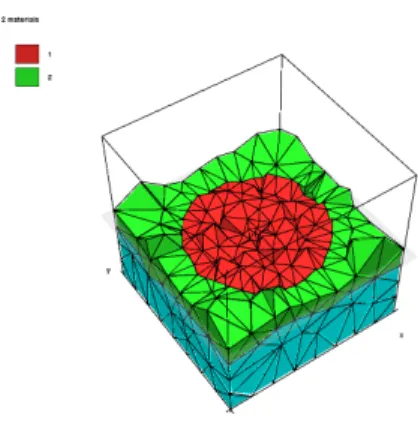
In the case of prostate, I define the regions under the guidance of physicians; in general, this step can be left to the users with knowledge in the target applications. In my examples, the prostate is naturally divided into two parts by the prostatic urethra, as shown in Fig. 3.4. My multi-region elasticity parameter estimation is aimed at determining which part of the organ of interest is stiffer and therefore more likely to have cancers. This work will assist in diagnosing cancer and in performing simulation-guided biopsy and other surgical procedures.
Figure 3.4: The Prostatic Urethra. The prostatic urethra naturally divides the prostate into two parts. © Wikipedia(Gray, 1918)
I choose to simulate the regions of the deformable body as one deformable body. I do this because I need to maintain the continuity of the surface of the target organ. Multi-region elasticity parameter reconstruction requires some modifications to the objective function defined in Eqn. 6.12. In this type of multi-region reconstruction, I use the following objective function:
Φ(µ) =
M X
m=1
X
vl∈Sm,l
with M as the total number of regions,Sm,las the deformed surface of themthregion, andSm,t as
the surface of the referencemthregion. The definition ofS
m,lis critical for the convergence of the
reconstruction.
I exclude the nodes that are shared by other regions (as shown in Fig. 3.5(a) and Fig. 3.5). When the nodes shared by the regions are included in the objective function given in Eqn. 3.13, the distancedH(vl,Sm,t)may lead to optimization in the wrong direction; the decrease in the distance
that is computed from these nodes’ displacement fails to show that the optimizer is converging to the ground truth. In fact, it is possible for the distance between the nodes and the reference surface to decrease while the optimizer isdivergingfrom the ground truth when nodes shared between regions are used in the computation. I address this issue by including only the original vertices on the surface of the object, not those on the shared boundary of two regions, as thevlin Eqn. 3.13. With
this approach, my experiments indicate that the multi-region parameter estimation can converge to the right parameters for each region simultaneously.
Region'1' Region'2'
(a) (b)
Figure 3.5: The 2D and 3D Illustration of the Nodes of Regions. (a) These nodes do not contribute to the convergence of the optimization. (b) The figure on the left shows nodes shared by the two regions; the figure on the right shows the nodes not shared by the two regions.
3.2.2.6 The Inverse Step
This step estimates the recovered elasticity parameters of the target organ (or tissue). It determines the accuracy of the estimated parameter by measuring the Hausdorff distance between the (model) surface of the reference organ and that of the deformed organ, using the displacement computed by the forward simulation.
Optimization (PSO) method (Kennedy et al., 1995; Poli et al., 2007; Clerc, 2010), a population-based stochastic optimization method. This variant of the PSO method has the following advantages:
1. It can cope with a noisy objective function that has many local minima;
2. it does not need to compute the gradient of the objective function; and 3. it is easy to parallelize the state updates of each particle.
Each particle in the PSO method corresponds to a state in the optimization process, and each particle possesses five attributes: the position, the velocity, the fitness value, the previous best position of itself, and the previous best position of the entire particle swarm. I use the subscript ito index the particle in the swarm,pi to represent the previous best position of theith particle,
andpg,i to represent the previous best position of its neighbors. Superscripttdenotes the current
iteration. Position will be a vector ofN dimension represented asµt
i, andvti is the velocity of the
ithparticle in the current iteration;yt
i (scalar value) represents the fitness value of theith particle in
the current iteration. The swarm size isM, which usually ranges from10to100. The dimensionN of the particle position and velocity is the same as the dimensionality of the optimization problem space. The five attributes of theithparticle at thetthoptimization iteration can then be defined as:
1. The positionµt
i = (µt1,i, . . . , µtn,i, . . . , µtN,i), withµit∈H,1≤n ≤N,1≤i≤M
2. The velocityvti = (v1t,i, . . . , vtn,i, . . . , vtN,i), withvmin ≤ kvtik ≤ vmax,1≤n≤ N,1≤i≤ M
3. The fitness valueyt
i = Φ(µti), withΦ()as the fitness function or the objective function of the
optimization problem
4. The previous best position of itselfpt
i = (pt1,i, . . . , ptn,i, . . . , ptN,i), withpti ∈H,1≤n ≤N,
1≤i≤M
The position is a point in the Euclidean search spaceHof the optimization problem. In my problem, the search space is the range of all possible elasticity parameters. The number of parameters I are recovering is the dimension of the search space of the optimization. In other words, the positions of the particles are a set of the parameters I want to estimate. The fitness value is computed from the fitness functionΦ, which is the objective function of the optimization problem (Eqn. 6.12). The velocity represents the search direction. The previous best position of the particle itself is the best set of parameters this particle has found so far. And the previous best position of its neighbors is the best set of parameters the neighbors of particles has found. The current position, the current velocity, the fitness value, the previous best position itself, and the previous best position of the swarm will be used to compute the velocity or the search direction.
Instead of optimizing one estimated solution at a time, a number of the particles are used together to collectively search for the best solution to the optimization problem (i.e., multiple coordinated searches going on simultaneously). Intuitively, the “particle swarm” will not only accelerate the search for the best solution, but will also increase the probability of finding the globally optimal solution.
The PSO method works by iteratively updating the particles’ properties. ThecanonicalPSO method uses the following two equations to update particle position and velocity, withRand()as a random value generator.
v(it+1) =vti+Rand()(pti−µti) +Rand()(ptg,i−µti) (3.14)
µ(it+1) =µti+vti+1∆t, (3.15)
with∆t = 1. The particle’s position update (Eqn. 3.14, Eqn. 3.15) can be computed since it is determined by several factors: the current positionµt
i; the persistence in the previous direction (first
part of Eqn. 3.14); the influence of the previous best position of itself (second part of Eqn. 3.14); and the influence from its neighbors (third part of Eqn. 3.14). Two questions remain:
2. how to weigh the particle’s persistence in its previous direction and the influence from its neighbors (i.e., how to refine Eqn. 3.14).
The design of appropriate PSO variants mainly focuses on these two issues.
Population Structure: The population structure of the swarm affects the convergence rate, as the structure determines how fast information propagates inside the swarm. If each particle in the swarm is informed by every other particle, the influence term in Eqn. 3.14 will be same for every particle, meaning that all particles will move in similar directions. This makes it easy for the swarm to become entrapped in a local minimum. But if each particle in the swarm is only informed by one or two other swarm particles, the influence of other particles will be small. But if the particles are not informed enough, this slows down the process of finding the best solution. Therefore, the way that information is communicated from particle to particle can be crucial. Various kinds of swarm topology, or population structures (Kennedy and Mendes, 2002), have been studied. The canonical particle swarm optimization (Eqn. 3.14, Eqn. 3.15) uses the global best solution so far; it connects every particle with every other particle. After some experiments, I chose instead to use the adaptive random structure (Clerc, 2012). With this adaptive scheme, after every unsuccessful iteration, the neighbors of the particleichanges toK random neighbors. This adaptive random structure keeps the particles informed about different neighbors at every iteration. The value ofKdepends on the swarm sizeM and the properties of the objective function. For my problem, I choseK = 3and M = 40based on my experiments.
Velocity: The canonical way of updating velocity (dimension by dimension) is known to be biased (Monson and Seppi, 2005). Therefore, I adapted the method of computing the velocity or the search direction from (Clerc, 2012). For each iteration, I update the velocity of theithparticles by
v(it+1) =C(vti,pti −µti,ptg,i−µti). (3.16)
The functionC, denoting the velocity of the next iteration, is dependent on three terms: (a) the current velocityvt