LOW-BACKGROUND GERMANIUM RADIOASSAY FOR THE MAJORANA COLLABORATION
James E. Trimble, Jr.
A dissertation submitted to the faculty at the University of North Carolina at Chapel Hill in partial fulfillment of the requirements for the degree of Doctor of Philosophy in the
Department of Physics.
Chapel Hill 2016
c 2016
ABSTRACT
James E. Trimble, Jr.: Low-background Germanium Radioassay for theMajorana Collaboration
(Under the direction of Reyco Henning)
The focus of the Majorana Collaboration is the search for nuclear neutrinoless double beta decay. If discovered, this process would prove that the neutrino is its own anti-particle, or a Majorana particle. Being constructed at the Sanford Underground Research Facility, the Majorana Demonstrator (MJD) aims to show that a background rate of 3 counts per region of interest (ROI) per tonne per year in the 4-keV ROI surrounding the 2039-keV Q-value energy of 76Ge is achievable and to demonstrate the technological feasi-bility of building a tonne-scale Ge-based experiment. Because of the rare nature of this process, detectors in the system must be isolated from ionizing radiation backgrounds as much as possible. This involved building the system with materials containing very low levels of naturally-occurring and anthropogenic radioactive isotopes at a deep underground site. In order to measure the levels of radioactive contamination in some components, the Majorana Demonstrator uses a low background counting facility managed by the Ex-perimental Nuclear and Astroparticle Physics group at UNC.
232Th were found, but all were orders of magnitude below the acceptable threshold for the
MJD. Also discussed is a proposed ultra-low background system designed to utilize technol-ogy designed for the MJD. Finally, a discussion is presented on the design and construction of an azimuthal scanner used by the Majorana Collaboration.
ACKNOWLEDGEMENTS
To Reyco, thanks for all the guidance, direction, knowledge...and putting up with the stupid questions. It was a blast!
Thank you to my daughters, Kate and Riley, for all the opportunities to edit this late at night and being my test audience for presentations. And to Penny for keeping me company during all day writing sessions.
I would also like to thank Flash Gordon. For saving every one of us.
Finally to my wife, Heather, you are the reason that I came back to school. Thank you for asking about going back to West Point over sushi at Taca in Savannah!
TABLE OF CONTENTS
LIST OF TABLES . . . ix
LIST OF FIGURES . . . x
LIST OF ABBREVIATIONS AND SYMBOLS . . . xiii
1 Introduction . . . 1
1.1 Motivation . . . 1
1.2 Majoranaand Neutrino Science . . . 1
1.2.1 History of Neutrino . . . 1
1.2.2 Solar Neutrino Problem . . . 5
1.2.3 Neutrino Oscillations . . . 6
1.2.4 Double Beta Decay and the Majorana Demonstrator . . . 9
1.3 Low-background Counting Overview . . . 12
1.3.1 History of Low Background Counting Systems . . . 12
1.3.2 History of Germanium Detectors . . . 12
1.3.3 Low-background Counting Facilities . . . 15
1.3.4 Low-background Radioassay Techniques . . . 17
2 Experimental Setup . . . 19
2.1 Introduction . . . 19
2.2.1 Natural Radioactivity of the Detector . . . 20
2.2.2 Natural Radioactivity of the Shielding / Radiation from the Activity of the Rock Walls and Laboratory Construction Materials . . . 20
2.2.3 Radioactivity in the Air Surrounding the Detector / Components of Cosmic Radiation . . . 21
2.3 Detector Principles of Operation . . . 23
2.4 Kimballton Underground Research Facility . . . 25
2.4.1 Facility overview . . . 25
2.4.2 UNC at KURF . . . 26
2.4.3 Data Acquisition System . . . 27
2.4.4 Detector Rehabilitation . . . 34
3 Neutron Activation for the Majorana Collaboration . . . 38
3.1 Introduction . . . 38
3.2 Sample Preparation . . . 39
3.3 Measurement . . . 42
3.4 Analysis . . . 47
3.5 Results . . . 52
4 Stainless Steel Flange Assay . . . 58
4.1 Introduction . . . 58
4.2 Measurement & Simulations . . . 58
4.3 Analysis & Results . . . 61
5 Conceptual Design and Simulations for an Ultralow-background
Ra-dioassay System . . . 68
5.1 Conceptual Design . . . 68
5.1.1 Front-end Electronics . . . 68
5.1.2 Electroformed Copper . . . 70
5.1.3 Larger Germanium Crystal . . . 73
5.1.4 Location of System . . . 73
5.2 Simulations . . . 74
6 Summary . . . 81
Appendix A Azimuthal Scanning Table . . . 83
A.1 Background . . . 83
A.2 Design modifications . . . 83
LIST OF TABLES
1.1 List of Neutrino Mixing Angles, their associated source, and experiments
fo-cused on each source. . . 7
1.2 List of low background counting facilities discussed in this section. . . 16
2.1 Values published for the Fano factor in germanium. . . 25
2.2 Specifications for both detectors managed by UNC at KURF. . . 27
3.1 Isotopes observed in neutron activation and their most intense emittedγ-rays used in neutron activation analysis. . . 39
3.2 Activation times and duration for standards and samples. All times are East-ern Standard Time. . . 42
3.3 Results of neutron activated analysis of 238U and 232Th standards. . . 56
3.4 Results of neutron activated analysis of 0.002-in PTFE and FEP tubing samples. 56 3.5 Results of neutron activated analysis of 0.005-in PTFE sample. . . 57
3.6 List of additional isotopes detected in the samples. . . 57
4.1 Isotopes observed in the sample and their most intense emittedγ-rays. . . . 67
5.1 Activities levels found in high purity commercially available copper specially selected for theMajorana Demonstrator . . . 72
5.2 Activities levels found in copper used in the copper shield for theMajorana Demonstrator [1]. . . 73
LIST OF FIGURES
1.1 Graph depicting a typical background spectrum for a shielded HPGe detector at the surface compared to the background spectrum for 2-neutrino double
beta decay and neutrino-less double beta decay. . . 2
1.2 Solar neutrino energy spectrum for a standard solar model. . . 6
1.3 Schematic drawing of the Majorana Demonstrator shown with both modules installed. . . 11
1.4 Pulse-height spectrum from a p-i-n junction in germanium due to 663 keV γ-rays from137Cs. . . 13
1.5 57Co spectrum obtained with 437-3 coaxial detector, linear scale. . . . . 14
1.6 Basic instrumental components of an ICP mass spectrometer. . . 18
2.1 Flux of cosmic ray secondaries and tertiary-produced neutrons in a typical Pb shield vs shielding depth. . . 22
2.2 Drive-in entrance to the Lhoist limestone mine where KURF is located on the 14th level. . . 26
2.3 Graph depicting the linear attenuation coefficient of germanium and its com-ponent parts. . . 28
2.4 Radioactive decay chain for238U. . . 29
2.5 Radioactive decay chain for232Th. . . . . 30
2.6 Circuit diagram and output shape for an integrated CR+nRC circuit. . . . 32
2.7 Block diagram of the DAQ system forMelissa and VT-1. . . 33
2.8 Vacuum pumping setup for VT-1. . . 35
2.9 Inside of VT-1 HV filter. . . 36
2.10 Inside of inhibit shutdown logic adapter box allowing the HV source for Melissato be connected safely to VT-1 and controlled remotely. . . 37
3.1 PULSTAR research reactor at North Carolina State University. . . 40
3.2 Table of masses for neutron activated samples and standards. . . 41
3.4 238U standard inMelissa . . . 44
3.5 232Th standard in VT-1 . . . . 45
3.6 238U standard spectrum in Melissa . . . 45
3.7 238U standard spectrum in Melissashowing a peak at 106 keV. . . 46
3.8 232Th standard spectrum in Melissa. . . 46
3.9 232Th standard spectrum in Melissa showing the dominant peak at 312 keV. 47 3.10 PTFE samples in Melissa . . . 48
3.11 FEP tubing sample in VT-1 . . . 49
3.12 Background spectrum for Melissa over a 24-hour period. . . 50
3.13 Background spectrum for VT-1 over a 24-hour period. . . 50
3.14 232Th standard spectrum in Melissa showing Gaussian and linear functions fit. . . 51
3.15 0.002-in PTFE sample spectrum in Melissa. . . 53
3.16 0.002-in PTFE sample spectrum in Melissashowing ROI around 106 keV. 53 3.17 0.002-in PTFE sample spectrum in Melissashowing ROI around 311 keV. 54 3.18 FEP tubing sample spectrum in VT-1. . . 54
3.19 FEP tubing sample spectrum in VT-1 showing ROI around 106 keV. . . 55
3.20 FEP tubing sample spectrum in VT-1 showing ROI around 311 keV. . . 55
4.1 Stainless steel flange used by the Majoranacollaboration. . . 59
4.2 SS flange inMelissa . . . 60
4.3 SS flange spectrum in Melissa . . . 63
4.4 SS flange spectrum forMelissa at 1120 keV . . . 64
4.5 Background spectrum forMelissa . . . 64
4.6 Background spectrum forMelissa at 1120 keV . . . 65
5.1 LMFE mounted in EFCu spring clip. . . 69
5.2 Crystal mount used in the Majorana Demonstrator with an LMFE in place on the top. The mount is made of electroformed copper which is dis-cussed in the next section. . . 70
5.3 MDA as a function of the efficiency of a Ge detector for gamma-rays with energy of ˜800 keV relative to a detector with 50% RE. . . 74
5.4 Geant4 simulation of new system. . . 76
5.5 Simulated spectrum in proposed system due to 214Bi and 208Tl. . . . . 77
5.6 Simulated spectrum in proposed system due to 214Bi and 208Tl. . . 77
5.7 Simulated spectrum in proposed system due to 214Bi and 208Tl. . . . . 78
5.8 Background at key gamma-line energies used in assay using an OFHC copper inner shield. . . 79
5.9 Background at key gamma-line energies used in assay using an EFCu copper inner shield. . . 79
5.10 Background at key gamma-line energies used in assay using an EFCu inner shield, crystal mount, and coldplate. . . 80
A.1 Technical drawing of azimuthal scanning table. . . 84
LIST OF ABBREVIATIONS AND SYMBOLS
0νββ Neutrinoless Double-beta Decay
2νββ Double-beta Decay C.L. Confidence Level
ENAP Experimental Nuclear and Astroparticle Physics HPGe High Purity Germanium
KURF Kimballton Underground Research Facility LBC Low Background Counting
PPC P-type Point Contact Q End-point Energy ROI Region of Interest
CHAPTER 1: Introduction
Section 1.1: Motivation
The focus of theMajoranaCollaboration is the search for the nuclear neutrinoless dou-ble beta decay (0νββ) of76Ge [2]. If discovered, this process would prove that the neutrino
is its own anti-particle or a Majorana particle [3–6]. Located in Lead, SD, the Majorana Demonstrator is being constructed on the 4850-ft level of the Sanford Underground Re-search Facility (SURF). TheMajorana Demonstrator aims to show that a background rate of 3 counts per ROI per tonne per year in the 4-keV ROI surrounding the 2039-keV76Ge Q-value energy, as shown in Figure 1.1, is achievable and to demonstrate the technological
feasibility of building a tonne-scale Ge-based experiment. Because of the nature and rarity of this process, detectors in the system must be isolated from ionizing radiation backgrounds as much as possible. This involves building the system with materials containing very low levels of naturally-occurring and anthropegenic radioactive isotopes and a deep underground site. In order to measure the levels of radioactive contamination in some components and determine if they can be used in the MJD, theMajorana Demonstratoruses a low back-ground counting facility managed by the Experimental Nuclear and Astroparticle Physics group at UNC.
Section 1.2: Majorana and Neutrino Science
1.2.1: History of Neutrino
Figure 1.1: Graph depicting a typical background spectrum for a shielded HPGe detector at the surface compared to the background spectrum for 2-neutrino double beta decay and neutrino-less double beta decay [7]. Note that the neutrino-less signal is magnified by 100. The half-life for this signal is approximately 1027 years which corresponds to a value of less
particle, or an electron, as shown here:
AÑB`e´ (1.1)
where A is the parent nucleus and B is the daughter nucleus. The underlying process that we now understand to be a neutron decaying into a proton was not known at the time as the neutron had not been discovered. At that time, however, an analysis of the kinematics and spin statistics of the process was made and a problem arose [8]. If one assumed the parent nucleus at rest and the two products of the decay were emitted in opposite directions to conserve momentum, it was assumed that one could use conservation of energy to calculate the kinetic energy of the emitted electron with
E “ ˆ
m2
A´m2B`m2e
2mA
˙
c2 (1.2)
wheremA is the mass of the parent nucleus,mB is the mass of the daughter nucleus, andme
is the mass of the emitted electron. This did not hold true, however, as experiments showed electrons emitted during beta decay are emitted at a range of energies. Equation 1.2 merely shows the maximum energy allowed for the electron. Physicists were unsure what accounted for the missing energy. Then in 1930, Wolfgang Pauli suggested that there might be another particle emitted in the process which carried off this as yet unaccounted for energy [8]. First proposing that the particle be called the “neutron" as it had to be electrically neutral, the name of “neutrino" or “little neutron" was settled upon after the discovery of the neutron by James Chadwick in 1932 [9]. Although skeptical at first, scientists widely accepted the neutrino after the publication of Enrico Fermi’s Theory of Beta Decay in 1934 [10].
detect a free neutrino [11]. Realizing that nuclear reactors were a reliable and large source of neutrinos, or more specifically anti-neutrinos, they proposed to put a detector near a reactor and use inverse beta decay to detect the reaction:
¯
ν`pÑn`e´ (1.3)
Two tanks of water were located underground near the reactor. The tanks contained 200 liters of water and were placed between three liquid scintillation detectors [12]. Anti-neutrinos from the reactor interacted with the protons in the water and created neutrons and positrons. The positrons were slowed down by the water and annihilated with electrons. This annihilation would emit two gamma rays per interaction which entered the liquid scintillators and created scintillation photons after interacting with atomic electrons. These photons were recorded by photomultiplier tubes mounted around the detectors. As confirmation of the neutrino detection, they doped the water tanks with cadmium chloride [11] which, as a neutron absorber, reacted as
n`108Cd Ñ109mCd (1.4)
109mCd
Ñ109Cd`γ1s (1.5)
The gamma rays emitted from the reaction created photons in the liquid scintillator as well, but with a delayed response caused by the thermalization time of the neutrons („9 µs). This allowed Cowan and Reines to confirm that the signals they were detecting were
1.2.2: Solar Neutrino Problem
Solar neutrinos are created primarily through the proton-proton chain (p-p chain) re-action in the Sun [14]. Two protons combine to form a hydrogen nucleus, a positron, and an electron-neutrino. This begins a chain reaction which creates more neutrinos and this production rate and corresponding flux at Earth, shown in Figure 1.2, was first calculated by John Bahcall in 1964 [15]. In the late 1960’s, Ray Davis designed and built the Homestake Experiment in order to measure the solar neutrino flux [16].
The experiment, built underground in the Homestake Mine located in Lead, SD, was based on the principle of neutrino capture, or inverse beta decay in chlorine,
νe`37ClÑ37Ar`e´ (1.6)
A 400,000-gallon tank of the pure liquid percholoroethylene, C2Cl4, was placed deep
un-derground to avoid the production of 37Ar in the detector by cosmic rays [16]. After the
tank was left for 100 days to allow 37Ar to reach a saturation point (t 1{
2 “ 35.02 days
[17]), it was flushed from the tank using helium gas. When measurements were made and compared to theoretical predictions, it was found that there were approximately one-third the number of neutrinos than expected. This surprising, and at the time controversial [18], result became known as the “Solar Neutrino Problem". The controversy was whether the discrepancy between calculated and measured solar neutrino counts was from incorrect stan-dard solar models, a misunderstood detector response, or neutrino oscillations. Subsequent experiments also saw the deficiency in solar neutrinos. SAGE (Soviet-American Gallium Experiment) measured solar neutrinos through the inverse beta decay reaction:
νe`71GaÑ71Ge`e´ (1.7)
Figure 1.2: Solar neutrino energy spectrum for a standard solar model [21]. Isotopes shown on the plots correspond to different reactions in the Sun. The Homestake Experiment was most sensitive to the 8B reaction.
solution to the solar neutrino problem came in the form of neutrino oscillations as shown later.
1.2.3: Neutrino Oscillations
First theorized by Bruno Pontecorvo in 1958 [22], neutrino oscillations were forwarded as a solution to the Solar Neutrino Problem. Similar to the Cabibbo-Kobayashi-Maskawa matrix for quark mixing [23, 24], neutrino oscillations are described using the Pontecorvo-Maki-Nakagawa-Sakata (PMNS) matrix [25] shown in Equation 1.8,
U “ ¨ ˚ ˚ ˚ ˚ ˝
c12c13 s12c13 s13e´iδ
´s12c23´c12s13s23eiδ c12c23´s12s13s23eiδ c13s23
s12s23´c12s13c23eiδ ´c12s23´s12s13c23eiδ c13c23
˛ ‹ ‹ ‹ ‹ ‚ ¨ ˚ ˚ ˚ ˚ ˝
eiα1{2 0 0
0 eiα2{2 0
0 0 1
˛ ‹ ‹ ‹ ‹ ‚ (1.8)
δ is a CP-violating phase term, and α1/α2 are called the Majorana phases and are only
meaningful if neutrinos are Majorana particles. The three mixing angles, θ12, θ23, and θ13,
are experimentally determined from solar, atmospheric, and reactor neutrinos respectively with additional constraints from accelerator-based experiments. Table 1.1 shows some of the experiments focused on measuring each type of neutrino and its associated mixing angle. As neutrinos propagate through space and mass eigenstates move in and out of phase with each other, neutrinos can oscillate from one flavor state to another. Assuming only two flavors participate in the oscillation, the probability that a neutrino of flavor`will oscillate to flavor `1 in a flight distance L is given by:
Ppν` Ñν`1‰`q “sin22θsin2 „
1.27|∆m2ji|peV2q Lpkmq
EνpGeVq
(1.9)
where∆m2ji is the mass squared difference between two neutrino flavors [26]. If the neutrino did not have mass, then all flavors would move at the same speed (the speed of light) from a source and would therefore never be out of phase. Neutrino oscillations were first conclusively shown to be the solution to the solar neutrino problem by both the Super-Kamiokande Collaboration and the Sudbury Neutrino Observatory Collaboration, which recently shared the Nobel Prize in Physics in 2015 “for the discovery of neutrino oscillations, which shows that neutrinos have mass [13]."
Mixing Angle ν-type Experiments
θ12 Solar SNO[27], Gallex/GNO[20], SAGE[19]
θ23 Atmospheric Super-K[28]
θ13 Reactor Daya Bay[29], Double Chooz[30], RENO[31]
Table 1.1: List of Neutrino Mixing Angles, their associated source, and experiments focused on each source.
cosmic ray protons and helium nuclei with nuclei in the upper atmosphere. Their flux at the surface of the Earth should be isotropic because their probability of interacting while traveling through the Earth is negligible. The SK detector was able to detect and differen-tiate between electrons and muons produced by the charge current (CC) interaction inside the detector of electron- and muon-neutrinos respectively. By determining the direction of travel for the resultant electrons and muons in the detector, SK was able to determine the direction of the incident neutrinos. Researchers were able to show that although the flux of electron-neutrinos were independent of direction, the flux of down-going muon-neutrinos vastly outnumbered the up-going muon-neutrinos. Since there was no change in the flux of electron-neutrinos, the muon-neutrinos must have oscillated into another flavor [32].
While SK measured atmospheric neutrinos, the Sudbury Neutrino Observatory (SNO) Collaboration was focused on solar neutrinos. SNO was a heavy water Cherenkov detector which consisted of 1,000 tons of ultra-pure heavy water (D2O) observed by 9,500 20-cm
diameter photomultiplier tubes submerged in light water [33]. Using the interactions shown here:
νe`2HÑe´`p`p pCCq (1.10)
νx`2HÑνx`p`n pNCq (1.11)
νx`e´ Ñνx`e´ pESq (1.12)
SNO detected 8B solar neutrinos generated from reactions in the Sun. The charge current
to that of the CC interaction, SNO provided evidence of flavor oscillation with no reference to solar model flux calculations [34]. SNO was able to report that of their measured total neutrino flux of5.09`0.44
´0.43pstatq `0.46
´0.43psystqˆ10
6cm´2s´1, the non-electron-neutrino component
was3.41`0.45 ´0.45pstatq
`0.48
´0.45psystq ˆ106 cm´2s´1 [33]. These values show that approximately
two-thirds of the neutrinos arriving from the Sun are not electron-neutrinos and therefore must have oscillated from an electron-neutrino while in transit to Earth since all solar neutrinos are produced as electron-neutrinos.
1.2.4: Double Beta Decay and theMajorana Demonstrator
Though much has been discovered about neutrinos, fundamental questions remain. One question is whether the neutrino is a Dirac or Majorana particle, i.e. its own anti-particle. Neutrinoless double-beta decay (0νββ) is one way to determine this. A rare transition between two nuclei, double beta decay occurs between two nuclei with the same mass number and a difference of two units of nuclear charge [35]. It only happens when the initial and final nuclei are more bound than the intermediate nucleus and can only occur for even-even nuclei. Since single beta decay is forbidden or strongly suppressed for these nuclei, they can undergo two neutrino double-beta decay (2νββ):
A
ZX ÑAZ`2X`2e´`2¯νe (1.13)
which was first theorized by Maria Goeppert-Mayer in 1935 [36]. In this decay, total lepton number is conserved and it is allowed in the Standard Model. First seen in the laboratory in 1950 [37] based on geochemical arguments, the decay has typical half-lives of 1018 - 1020
double-beta decay [39]:
A
ZX Ñ
A
Z`2X`2e
´
(1.14)
This decay mode violates lepton number conservation and is forbidden by the Standard Model. Both 2νββ and 0νββ are second-order weak processes which mean they occur with a long lifetime. One key difference between the two decays modes, however, is the energy spectrum created. The2νββ decay mode electron kinetic energy spectrum is continuous and peaks below 1
2Qββ, where Qββ is the Q-value of the reaction [35]. 0νββ can be found by
searching the spectrum of the summed energy of the emitted betas for a monoenergetic line at the Q-value of the decay [35] as shown in Figure 1.1.
TheMajoranaexperiment seeks to uncover the nature of the neutrino through a search for 0νββ using 76Ge. In support of this search, the Collaboration has constructed the Ma-jorana Demonstrator to show that backgrounds can be made low enough to justify construction of a large double beta decay experiment using enriched high purity enriched Ger-manium (HPGe) [40]. Constructed at the Sanford Underground Research Facility (SURF), the Demonstrator is located in the Homestake Mine in Lead, SD. Due to the extraor-dinarily low ionizing radiation backgrounds required, extreme efforts have to be made to minimize the background contributions from both the local environment and detector ma-terials. The main aspects of the apparatus materials are summarized as follows [40, 41] and shown in Figure 1.3:
• Natural radioactive impurities were removed from the germanium crystals through enrichment, zone refining, and crystal growth.
Figure 1.3: Schematic drawing of the Majorana Demonstratorshown with both mod-ules installed [1]. The different layers of the shield are indicated in the drawing. The outer surface of the inner Cu shield is 50.8 cm in height and 76.2 cm in length.
• Modern lead was used outside the copper shielding. The lead was sufficiently pure to be employed as the main outer shield.
• Electrical and thermal shielding was achieved using different high purity plastics. In particular, polytetrauoroethylene (PTFE) was used in several places and its assay is discussed later in this thesis.
• Due to the proximity to the detector, front-end electronics were designed to be low-mass and ultra-low background.
• Extremely low-mass miniature coaxial cables were used for signal and high-voltage.
Section 1.3: Low-background Counting Overview
1.3.1: History of Low Background Counting Systems
The true starting point for low-level radioactivity measurement is traced back to the discovery of 14C dating techniques. In 1949, scientists successfully demonstrated that 14C
could be used to effectively date samples and validated their discovery by comparing their results to old samples with ages on the order of the half-life of14C (t1{
2 “5700y[17]) [42, 43].
Low-level or low-background is presently understood to refer to both activities that can barely be measured and to intrinsic radioactivities occurring naturally in the environment [44]. Germanium detectors are particularly effective for measuring bulk activities and are widely used in the low background community to conduct bulk low-level radiopurity measurements for reasons discussed in Chapter 2.
1.3.2: History of Germanium Detectors
First theorized in 1960, the lithium-drift process was used to manufacture the first Ge-detectors [45]. This process was used by Freck and Wakefield in 1962 to make the Ge-detector that generated the first everγ-ray spectrum from a lithium-drifted Ge-diode shown in Figure 1.4. The small crystal used (approximately 0.75 cm3) had poor resolution (3% at 662 keV) [46], but proved that the detector concept was valid. An improvement was presented a year later by Tavendale and Ewan with a resolution of 0.45% at 1332 keV, which gave Ge-detectors a better resolution that NaI-detectors [47]. One drawback to the Li-drifted detectors was the requirement to be kept at cryogenic temperatures at all times. This vulnerability was due to the lithium charge carrier being sufficiently mobile at room temperature to cause a redistribution of lithium [48]. However, in 1971, Hall and Soltys proposed the idea of a high purity germanium (HPGe) detector which would reduce the concentration of electrically active impurities to 1010 cm´3 [49]. A small concentration is necessary, however, as the
Figure 1.4: Pulse-height spectrum from ap-i-njunction in germanium due to 663 keVγ-rays from137Cs [46]. This is the first published spectrum generated from a germanium detector.
the detector. One year later this process would be used by Llacer to produce the first ever γ-ray spectrum from an detector [50] as shown in Figure 1.5. Since then, HPGe-detector has continued to improve its resolution and detection limits. Crystal manufacturing techniques have also allowed larger detectors to be made.
In order to compare the low background assay capabilities of one detector to another, one can use the minimum detectable activity (MDA). The MDA is found with [51]:
MDA “ 2.71`3.29
?
2BRˆtC ˆFWHMˆF
ˆPγˆtC
(1.15)
whereBR is the background count rate in counts per keV,tC is the count live time, FWHM
is the resolution of the detector, F is the statistical coverage factor based on the confidence level, and Pγ is the statistical probability of emitting a gamma-ray at a specific energy. Pγ,
Figure 1.5: 57Co spectrum obtained with 437-3 coaxial detector, linear scale [50]. This is the first published spectrum generated from a HPGe detector.
1.15 implies:
MDA 9
?
BRˆFWHM
REˆ?tC
(1.16)
By lowering the MDA, one would improve your sensitivity to contamination in a sample. One can see from Equation 1.16 that there are four possibilities to achieve this more sensitive detector:
• Lower BR by making the shielding sufficiently thick or reducing the radioactive
back-grounds of the construction materials. • Lower FWHM (improve energy resolution).
• Increase the relative efficiency by using a larger crystal or optimizing the shape of the sample around the detector crystal.
• Increase the count live time.
well, as shown by the MDA. If we examine the limit where the radioactive background has been lowered to effectively zero, Equation 1.15 instead reduces to:
MDA 9 2.71
REˆtC
(1.17)
As the MDA is now linear in time, one can now assay samples much faster. This is another reason for reducing the backgrounds; it allows for much faster assays of samples. However, while this is a factor that can be taken into account while conducting radioassay, increasing the relative efficiency is more effective if all other factors stay the same.
1.3.3: Low-background Counting Facilities
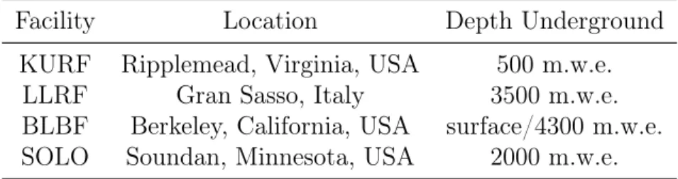
There are currently many low background counting facilities around the world using HPGe detectors, including KURF which is the focus of later chapters in this thesis. Though it does not list every facility in the world, Table 1.2 shows several of the most prominent ones and I will briefly discuss these here.
The LNGS (Laboratori Nazionali del Gran Sasso) maintains the LLRF (Low Level Re-search Facility) at a depth underground of 3800 m.w.e (meters of water equivalent shielding). The main detector used for low background counting is the GeMPI system [52]. GeMPI is a 2.2-kg crystal used in a detector mounted in a clean room environment at the lab. The system consists of shielding from inside to out:
• 5 cm high-purity copper (99.9975%) • 5 cm of Pb with 6 Bq/kg of210Pb • 10 cm of Pb with 20 Bq/kg of 210Pb
• 5 cm of Pb with 130 Bq/kg of 210Pb
shield protects the inner chamber from lab space air. The sample space is an approximately 151 in3 volume. The sample chamber is reached from the glove box antechamber by sliding
apart the top portion of the Pb and Cu shield that is mounted on bearings. Published sensitivities for GeMPI are 0.996 ppt for 238U, 0.999 ppt for 232Th, and 1.0 ppb [52].
Facility Location Depth Underground
KURF Ripplemead, Virginia, USA 500 m.w.e.
LLRF Gran Sasso, Italy 3500 m.w.e.
BLBF Berkeley, California, USA surface/4300 m.w.e. SOLO Soundan, Minnesota, USA 2000 m.w.e.
Table 1.2: List of low background counting facilities discussed in this section (m.w.e. ” meters of water equivalent) . KURF will be discussed in detail in a later chaper.
The Berkeley Low Background Facility (BLBF) is maintained by LBNL (Lawrence Berke-ley National Laboratory) in BerkeBerke-ley, California. They have two main systems; the first is a surface facility that has been in operation since the 1960’s [53]. It contains a 2.2-kg HPGe crystal that operates at an effective depth of 10 m.w.e. The walls of the facility are 1.5-meter thick portland concrete removing the necessity for thick Pb shielding. Measurements of the concentrations of U and Th in the concrete were on the order of the ppb level. A 3π muon veto system has assisted with lowering the detector’s radioactive backgrounds. Current sen-sitivities for the surface facility are 500 ppt for 238U, 2000 ppt for 232Th, and 1.0 ppm for
40K [54]. LBNL also maintains a second facility at SURF which operates at a depth of 4300
m.w.e. The underground facility has a 20-cm Pb shield with a Cu liner. It has a rolling lid that provides access to the 60 cm ˆ 60 cmˆ 60 cm sample chamber. Both facilities have a liquid nitrogen gas purge radon suppression system. Current published sensitivities for the underground facility are 50 ppt for 238U, 200 ppt for 232Th, and 100 ppb for40K [54].
of Doe Run Pb with a measured 210Pb activity of 50 Bq/kg. This outer shield surrounds a 2-in thick inner shield of 150-year old Pb with a measured210Pb activity of 50 mBq/kg. The
entire system is encased in two airtight layers of 50-µm thick mylar which is purged with liquid nitrogen boiloff to remove radon contamination. The system has two sample chambers (one for each detector) that each have an 8-in wide access port. Published sensitivities for SOLO are 0.1 ppb for U/Th and 0.25 ppm for K [56].
1.3.4: Low-background Radioassay Techniques
There are several techniques used in radiopurity measurements. As mentioned above, the three techniques used by theMajorana Collaboration were gamma-ray counting, neutron activation analysis, and ICP-MS. Gamma-ray counting and neutron activation analysis are discussed in detail in later chapters and are the focus of this thesis. We will discuss ICP-MS briefly here.
Figure 1.6: Basic instrumental components of an ICP mass spectrometer [60].
CHAPTER 2: Experimental Setup
Section 2.1: Introduction
In this chapter, I will discuss the overall experimental setup used throughout this thesis. We will begin by introducing the main types of radioactive background that may be present in low background radioassay and how to mitigate each one. I will then present the low back-ground counting lab at Kimballton Underback-ground Research Facility. After a brief overview of the facility, I will give a description of the hardware, software, and data acquisition systems for both detectors used. Finally, I will close with a description of some routine rehabilitation work that was conducted on both detectors in order to bring them up to functional status.
Section 2.2: Radioactive Background Reduction
Due to the ultra-low activities required for low-background experiments, detectors must be isolated from external forms of radioactivity as much as possible. There are five categories of background radiation [48]:
1. Natural radioactivity of the constituent materials of the detector itself
2. Radiation from the construction materials of the laboratory, rocks walls if in an un-derground location, or other far-away structures
3. Natural radioactivity of the ancillary equipment, supports, and shielding placed in the immediate vicinity of the detector
Each source of background radiation must be reduced as much as possible in order to get the most sensitive measurement of impurities in the sample.
2.2.1: Natural Radioactivity of the Detector
Germanium detectors are used in low-background radioassay for two main reasons: low inherent radioactivity and excellent energy resolution. This level of high purity is achieved by the use of a process called zone refining and crystal pulling. Zone refining starts with 98% pure germanium used in the semiconductor industry [48]. The crystal is locally heated inductively and the heated zone is passed along the length of a germanium bar. As the melted zone moves along the bar, local impurities which are more soluble in the molten germanium are preferentially transferred to the molten germanium and swept to the ends of the bar. This process, after many repetitions, can create impurity levels as low as 109 atoms
¨ cm´3 [48]. The subsequent crystal growing using a Czochralski puller can further remove
impurities, but not by orders of magnitude.
2.2.2: Natural Radioactivity of the Shielding / Radiation from the Activity of the Rock Walls and Laboratory Construction Materials
A large source of background radiation around a detector comes from the walls of the lab and the rock walls of the mine, if located underground. The primary shield used by most detectors against this radiation is an outer lead shield due to its high atomic number as well as it’s low Compton scattering to absorption ratio. This lead shield is responsible for shielding the detector from gamma-rays from the decay chains of238U,232Th, and40K in
[62]. 210Pb is in the decay chain of238U and the contamination of the lead shield with 210Pb usually comes from the U-rich lead ores used in the smelting process. However, the lead used to shield Melissa in this experiment came from Doe Run, Missouri, and was naturally low in U with a certified210Pb activity of less than 100 Bq ¨kg´1 [63].
The second form of shielding used in low-background experiments is an inner shield of a lower Z material. This lower Z material is used to shield the detector from interactions in the outer lead shield. Cosmic rays and gamma rays from radioactively decaying impurities in the outer shield interact with the lead causing additional Bremsstrahlung radiation or down-scattered gamma-rays. The Bremsstrahlung production rate is directly proportional to the square of the atomic number of the shielding material orZ2. This relationship is one driver
for using copper as an inner shielding material. By using the lower Z copper (ZPb “ 82,
ZCu “29), the inner shield now isolates the detector from a majority of the Bremsstrahlung
radiation. Copper can also be found with lower intrinsic levels of U and Th than lead. However, copper can contain radioactive contaminants as well. One way to minimize this contamination is by using commercially available oxygen-free highly conductive (OFHC) copper as the shield material. High purity commercially available OFHC copper can have activities as low as 1.25µBq¨kg´1 for U and 1.1µBq¨kg´1 for Th [1]. Additionally, copper exposed to cosmic rays will become activated with 60Co. This can be mitigated by moving
the copper shielding material underground as quickly as possible after manufacturing or performing underground electroforming of copper as discussed in a later chapter [40]. One other consideration is backgrounds from ancillary equipment, such as front end electronics and cables. These both need to be low background as well.
2.2.3: Radioactivity in the Air Surrounding the Detector / Components of Cosmic Radia-tion
Figure 2.1: Flux of cosmic ray secondaries and tertiary-produced neutrons in a typical Pb shield vs shielding depth. Neutron flux from antrual fission and (α, n) reactions is also shown. The nucleonic component is more than 97% neutrons [61].
neutrons, as well as pions, electrons, and protons. The secondary particles can cause a Bremsstrahlung radiation continuum in material around the detector, (n, γ) reactions, or direct ionization of the detector. Surrounding the detector with an active muon veto shield can reduce this background somewhat, however, this effect can be completely mitigated by placing the detector deep enough underground. As the cosmic radiation effects are focused almost directly downward at the surface of the Earth, placing a large rock overburden above the detector greatly reduces this effect. As shown in Figure 2.1, however, going further than 1000 m.w.e. underground brings no additional benefits for low background counting.
laboratories seeping in from the walls and surrounding rock. An underground lab with poor airflow can let the 222Rn accumulate where it will linger due to a half-life of 3.8 days [17].
The average concentration of 222Rn in the air is approximately 40 Bq
¨ m´3 [61], while concentrations at KURF range from 37 Bq ¨m´3 in winter to 122 Bq ¨ m´3 in the summer
[63]. This radon gas must be purged from the sample chamber. At the UNC LBC facility, liquid nitrogen boil-off is allowed to fill the sample chamber, flushing the area of 222Rn.
Section 2.3: Detector Principles of Operation
In radioassay systems such as the ones managed by UNC, germanium crystals are used to detect incident gamma rays at characteristic energies from samples in the vicinity of the detector. There are three possible interactions for a gamma ray entering a detector crystal: photoelectric absorption, pair production, and Compton scattering. As shown in Figure 2.3, each interaction is dominant in a specific range of incident gamma-ray energies. Photoelectric absorption is dominant at lower energies (À100 keV) and pair production becomes dominant at higher energies (Á 10000 keV). For most of the ROI for low-background assay using Ge detectors, however, Compton scattering is the dominant interaction.
energy [64]. By applying an electric field to the crystal, electrons and holes each move respectively along the electric field lines according to their effective charge. The drifting charges are collected at electrodes on the crystal surfaces and transferred to amplification electronics. For germanium, the number of charge carriers created is directly proportional to the energy deposited in the crystal, making it a very effective material for gamma-ray spectroscopy.
The energy resolution of a germanium detector can be found by calculating the full width at half maximum (FWHM) of a typical peak in the spectrum due to mono-energetic gamma-rays with the following equation
WT2 “WD2 `WX2 `WE2 (2.1)
whereW2
D is the inherent statistical fluctuation in the number of charge carriers created,WX2
is due to incomplete charge collection (statistically insignificant if the electric field is strong enough, i.e. matching the recommended bias voltage), and WE2 represents the broadening effects of all electronic components following the detector [48]. The statistical fluctuation in the number of charge carriers can be found with
WD2 “ p2.35q2F E (2.2)
where F is the Fano factor, is the energy required to create one electron-hole pair ( = 2.98 eV for Ge [64]), and E is the energy of the incident gamma ray. The Fano factor is the ratio of the observed statistical variance in the number of charge carriers from the expected number due to a Poisson model to the expected number of charge carriers or
F “ observed statistical varianceE
{
. (2.3)
therefore causing the deviation from Poisson statistics. Since 1967, there have been a range of values published for the Fano factor in germanium, some of which are shown in Table 2.1. The existing database of values tend to support two groups of values, one centered on 0.06 and another centered on 0.13 [65]. In his text, Knoll shows several of the values seen in Table 2.1, but quotes 0.08 as his assumed Fano factor [48]. Ultimately, the Fano factor contains information about atomic and molecular collisions as charged particles stop in matter, but these processes are very complicated and make the calculation of the Fano factor difficult. In this thesis, the resolutions for the detectors used were directly measured and not calculated, so a definite value for the Fano factor was not necessary.
Publication Energy Range
Author(s) Year Examined (keV) F
Bilger [66] 1967 122-4806 0.1288˘0.0024
Pehl and Goulding [67] 1970 8-1333 0.0791˘0.0028
Sher and Keery [68] 1970 662 «0.102
Zulliger and Aikten [69] 1970 60-122 «0.061 Strokan and others [70] 1971 583-1592 0.058˘0.0011
Owens [71] 1985 81-1333 0.0614˘0.0080
Croft and Bond [65] 1991 14-6129 0.112˘0.001 Table 2.1: Values published for the Fano factor in germanium.
Section 2.4: Kimballton Underground Research Facility
2.4.1: Facility overview
The Kimballton Underground Research Facility (KURF) is located in Ripplemead, VA, at the Kimballton mine operated by Lhoist North America. Facility operations are managed by the Virginia Polytechnic Institute and State University (VT). Located on the 14th level of
Figure 2.2: Drive-in entrance to the Lhoist limestone mine where KURF is located on the 14th level [72].
facility. Upon entering the mine, the lab is reached after an approximately two mile drive underground.
2.4.2: UNC at KURF
configuration [73]. VT-1’s shield consists of a 10.1-cm ORTEC commercial lead shield and 0.3 cm of OFHC copper. The sample cavity is cylindrical with dimensions 41 cm (height)ˆ 28 cm (diameter). The FWHM for VT-1 is 2.27 keV at 209.7 keV. Both assay cavities are continuously flushed with liquid nitrogen boil-off to purge radon gas. Further specifications for the detectors are given in Table 2.2.
Melissa VT-1
Manufacturer Canberra ORTEC
Relative efficiency 50% 35%
Performance
FWHM at 1.33 MeV (keV) 1.70 1.80
Threshold (keV) 20 20
Shield
Lead thickness (cm) 15.2 10.1
Oxygen-free high conductivity
(OFHC) copper thickness (cm) 2.54 0.3
Crystal (coaxial)
Mass (kg) 1.1 0.956
Length (mm) 64.5 75.7
Diameter ( mm) 65 55.8
Hole diameter (mm) 7.5 9.1
Hole depth (mm) 50 63.2
Outer electrode thickness (mm) 1.06 0.7
Inner electrode thickness (µm) 0.3 0.3
Cryostat
End cap diameter (mm) 82 70
End cap thickness (mm) 1.5 1.3
End cap to crystal (mm) 5 4
End cap material High Purity Al Mg
IR window material Al MylarTM, Kapton Al MylarTM Table 2.2: Specifications for both detectors managed by UNC at KURF [63].
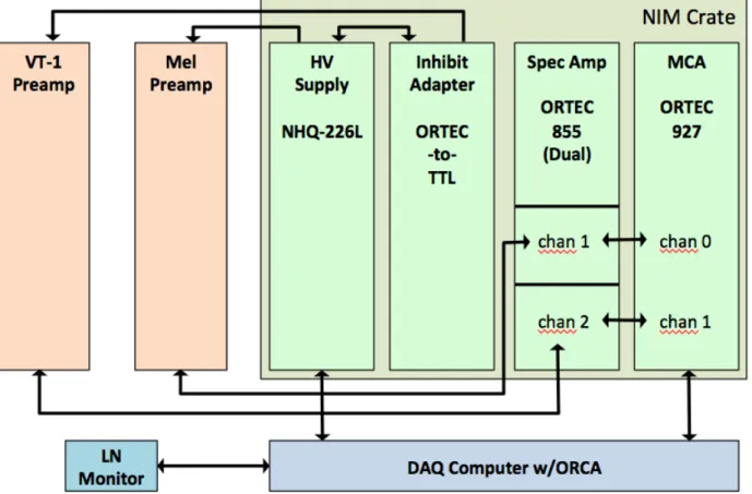
2.4.3: Data Acquisition System
Figure 2.4: Radioactive decay chain for238U [74]. The isotope with the most intense gamma-ray energy peaks is 214Bi at 609.3 keV, 1120.3 keV, 1238.1 keV, 1764.5 keV, and 2204.2 keV
bias supply provides the potential difference needed to generate an electric field inside the germanium crystal. This electric field is used to sweep the electron-hole pairs generated by incoming gamma rays out of the detector and be collected by the pre-amplifier [51]. These collected charges are converted into a voltage pulse and sent to the amplifier. While in the amplifier, the incoming charge pulse is shaped and amplified before being sent to the multi-channel analyzer (MCA). This shaping is done with a C1R1+n(R2C2) circuit as shown in
Figure 2.6 where CR is indicative of a high-pass filter and nRC stands for an “n" number of low-pass filters. These combinations of filters shape the incoming pulse into essentially a smoothed gaussian. The gaussian shape is required by the MCA to accurately measure the pulse height. This stream of shaped and conditioned pulses of varying height and spacing is sent to the MCA. At the MCA, the pulse heights are measured. Additionally, the MCA stores an internal histogram of pulse heights. In this way, the MCA is able to generate a spectrum viewable by the user.
Both detectors were biased via an ISEG NHQ-226L high voltage supply. The module is a 5-kV NIM mounted supply that allows the user to select polarity. Controlled by ORCA, the NHQ-226L can remotely bias and unbias both detectors. It also can automatically ramp down the bias voltage to zero in case of unexpected power loss or detector warming. Melissa is connected directly to the NHQ-226L, but VT-1 is routed through a custom built inhibit logic adapter due to a mismatch in shutdown logic discussed in the next section.
Liquid nitrogen levels for both detectors are monitored and controlled by an American Magnetics, Inc. (AMI) Model 286 liquid level controller (LLC). Two 240-L transfer dewars sit outside the shipping container housing the detectors and automatically refill the 30-L cooling dewars that keep the detectors cold as well as the boiloff dewar used to purge the sample chamber of radon. Levels can be viewed and controlled remotely via ORCA as well.
2.4.4: Detector Rehabilitation
Originally commissioned in 2011, the LBC lab at KURF had not been used since July 2014 and both detectors were non-operational and had to be repaired. In August 2015, both detectors were subjected to a thorough rehabilitation program with preventive maintenance while management of the facility was transferred from one graduate student to another. Melissa and VT-1 were warmed up and brought back to UNC to repump the cryo space vacuums on both detectors, a common maintenance requirement for HPGe detectors. The vacuum pump setup for VT-1 is shown in Figure 2.8.
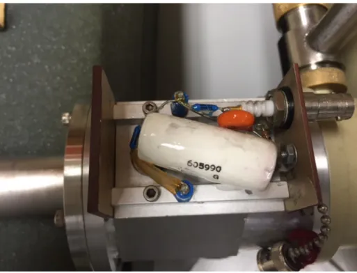
Figure 2.9: Inside of VT-1 HV filter. Note the grey residue on the large white capacitor.
Figure 2.10: Inside of inhibit shutdown logic adapter box allowing the HV source forMelissa to be connected safely to VT-1 and controlled remotely.
translates an ORTEC shutdown signal from VT-1 into a TTL signal that is accepted by the HV module, as shown in Figure 2.10.
CHAPTER 3: Neutron Activation for the Majorana Collaboration
Section 3.1: Introduction
Neutron activated samples of polytetrafluoroethylene (PTFE) and fluorinated ethylene propylene (FEP) tubing were γ-assayed in the LBC lab at KURF after they were neutron activated. These samples were tested due to their possible uses in the Majorana exper-iment. Specifically, PTFE is a candidate to be used as a gasket material for sealing the Majoranacryostat. FEP tubing is to be used as strain relief on signal cables into a D-sub connector. Neutron activation is utilized as a counting method when impurities in a sample may be at too low levels to detect with passive radioassay techniques. Samples are placed in a high neutron flux environment, such as a nuclear reactor, to be bombarded with energetic neutrons. Impurities in the sample capture a neutron, converting them to an unstable iso-tope, as shown in Equation 3.1 with 238U. This isotope in turnβ-decays to another isotope
shown in Equation 3.2 which emits characteristicγ-rays with well defined energies as shown in Table 3.1. These energies can be used to positively identify the presence of the emitting isotope and therefore the original impurity. Also, the isotopes which are created during neu-tron activation have a much shorter half-life than the238U impurity, which greatly increases
the decay rate and activity of that impurity. This renders the impurity detectable. Similar reactions used to identify 232Th impurities are shown in Equations 3.3 and 3.4.
238U
`n Ñ239 U˚ (3.1)
239U˚
Ñ239 Np`e´
232Th
`n Ñ233 Th˚ (3.3)
233Th˚
Ñ233 Pa`e´`ν¯e (3.4)
Impurity isotope: 238U 232Th Activation isotope: 239Np 233Pa
Half-life (days): 2.356 26.975 Relevant γ-ray for isotope (keV): 106 312
Intensity: 25.34% 38.5%
Table 3.1: Isotopes observed in neutron activation and their most intense emitted γ-rays used in neutron activation analysis.
Section 3.2: Sample Preparation
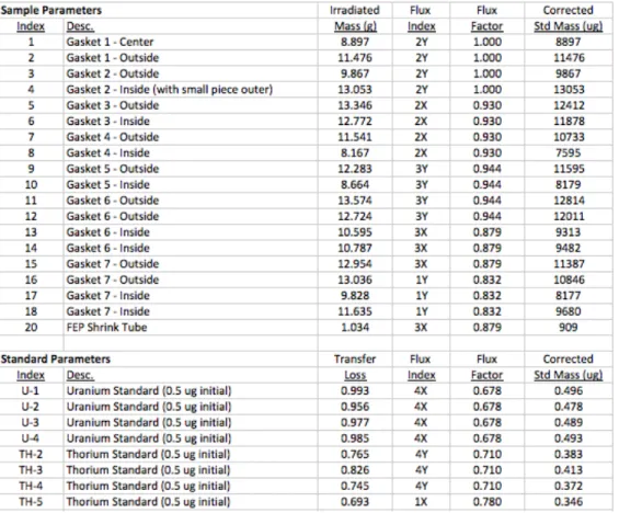
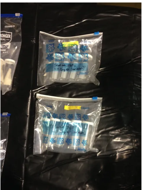
Thinly sliced PTFE samples and small sections of FEP tubing were activated at various times as shown in Table 3.2 at the PULSTAR high flux reactor at North Carolina State University as shown in Figure 3.1 [79]. Total time in the reactor over this period was 18 hours. Activated samples of varying masses as shown in Figure 3.2 were placed in plastic vials and packaged for shipping to Virginia Tech (VT). Ten vials containing 0.002-in thick PTFE samples were placed in a heat sealed plastic bag. This plastic bag was placed inside of a resealable plastic bag and labeled accordingly. Eight vials containing 0.005-in thick PTFE samples were placed in a heat sealed plastic bag along with the one vial containing FEP tubing. The samples arrived at VT on October 7, 2015. Environmental Health and Safety at VT received the samples and checked them for external contamination leakage. None was found and all samples demonstrated no more than 0.2 mrem/hr of activity externally. Samples were transported underground to KURF on October 7, 2015, and assays were started that day.
Date Time in Time out # of hours
9/30/15 10:44 12:53 2.15
9/30/15 13:03 16:14 3.18
10/1/15 10:13 16:30 6.28
10/2/15 9:28 15:51 6.38
Total # of hours: 17.99
Table 3.2: Activation times and duration for standards and samples. All times are Eastern Standard Time.
known uranium and thorium concentrations that were used to calibrate the spectra from the samples and to find the ratio between absolute U/Th levels in the samples and measured γ-ray activities. The standards were packaged in sealed plastic bags as well as shown in
Figure 3.3.
Upon arrival at the lab, a sample preparation station was arranged. A table was placed outside of the detector lab with a plastic sheet on top. Everything inside of the shipping container was treated as potentially contaminated. At all times, nitrile gloves were worn when handling anything that was inside the original shipping container or came in contact with something inside the shipping container. Two Marinelli beakers were designated for use in the detectors with the samples.
Section 3.3: Measurement
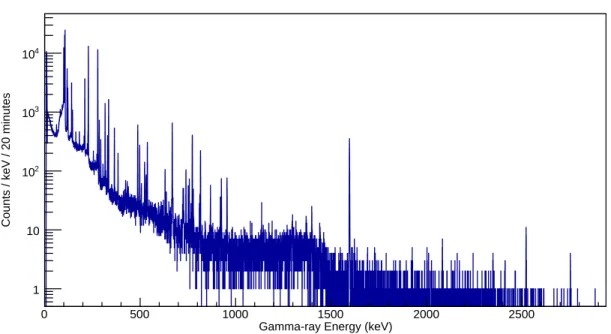
Measurements were made using the two detectors at the UNC low-background counting facility at KURF. Each set of standard vials were placed in one of the detectors for 20 minutes at a time. For the first 20 minutes, the 238U standards were placed in
Melissa as shown in Figure 3.4 and the 232Th standards were placed in VT-1 as shown in Figure 3.5.
in Figure 3.10 and the FEP tubing samples were placed in VT-1 for assay as shown in Figure 3.11. Emphasis was placed on these two samples at the request of Matt Green.
Figure 3.4: 238U standard in Melissa
Figure 3.5: 232Th standard in VT-1
Gamma-ray Energy (keV)
0 500 1000 1500 2000 2500
Counts / keV / 20 minutes
1 10 2 10
3 10
4 10
MELISSA U-238 Standard
Figure 3.6: 238U standard spectrum in
Gamma-ray Energy (keV)
85 90 95 100 105 110 115 120
Counts / keV / 20 minutes 103 4 10
MELISSA U-238 Standard
Figure 3.7: 238U standard spectrum in Melissa showing a peak at 106 keV due toβ-decay of the activation product 239Np. Peaks at 99.5 keV, 103.3 keV, and 117 keV are the k
α1, kα2,
and kβ1 x-rays from the decay of 239Np, repectively.
Gamma-ray Energy (keV)
0 500 1000 1500 2000 2500
Counts / keV / 20 minutes
1 10 2 10
3 10
4 10
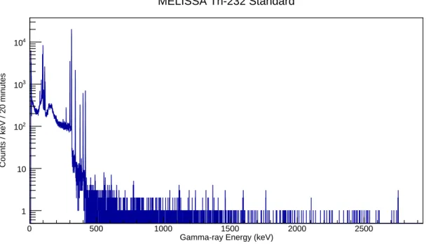
MELISSA Th-232 Standard
Gamma-ray Energy (keV)
270 280 290 300 310 320 330 340 350
Counts / keV / 20 minutes
1 10
2
10
3
10
4
10
MELISSA Th-232 Standard
Figure 3.9: 232Th standard spectrum in
Melissa showing the dominant peak at 312 keV due toβ-decay of the activation product 233Pa. The peaks at 271 keV, 300 keV, and 340 keV
are from the same decay.
Section 3.4: Analysis
The number of counts in the ROI for the standards were found by subtracting the back-ground from the peak in the ROI. Backback-ground spectra for Melissaand VT-1 are shown in Figures 3.12 and 3.13 respectively. A Gaussian function was fit to the peak in the spectra from the standards at the known energy which gave the mean (or centroid of the peak) and the standard deviation,σ, of the fit distribution. The ROI in this case was a region extending ˘3σ from the centroid of the peak in the standard. A Gaussian plus a linear function was then fit to a region extending 5σ on each side of the ROI. The linear portion of the fit was used to calculate the background as shown in Figure 3.14. This background was then applied to the ROI and subtracted from the peak area. Backgrounds in the samples measured were negligible. The result was the number of peak counts for that particular energy.
Gamma-ray Energy (keV)
0 500 1000 1500 2000 2500
Counts / keV / 24 hours
1 10 2 10
MELISSA Background
Figure 3.12: Background spectrum for Melissa over a 24-hour period.
Gamma-ray Energy (keV)
500 1000 1500 2000 2500 3000
Counts / keV / 24 hours
1 10 2 10
VT-1 Background
Run Time: 1 hours Entries 8192 Mean 312.4 RMS 1.17
Energy (keV)
304 306 308 310 312 314 316 318 320
Counts / keV
10 2 10 3 10 4 10
Run Time: 1 hours Entries 8192 Mean 312.4 RMS 1.17
MELISSA TH-232 Standard
Figure 3.14: 232Th standard spectrum in
Melissashowing Gaussian and linear functions fit to a region extending 5σ on either side of the ROI. Though the linear fit to the background does not match the background well, the background contributes 1% of the counts and introduces a negligible uncertainty.
as determined for a specific peak is:
Aγs “
N
mt (3.5)
whereN is the net peak area in counts at the energy observed with the background subtracted out, t is the assay live time, and m is the mass of U or Th in the standard. This rate was then used to find the initial standard decay rate for the isotopes of interest with:
Aos “Aγseλ ¯ t
(3.6)
whereAos is the initial activation decay rate,¯t is the average time since activation, andλ is
the decay constant for that isotope.
then required to be less than or equal to the upper limit, 90% C.L. - 1.65σ. We can convert this limit on the counts to a limit on the mass fraction of the isotope using the measured activities in the activated standards. This is given by:
Mass Fraction Limit“1.65
a Np
tmγ 1
Aos
eλ¯t (3.7)
where Np is the number of counts in the ROI for the sample, t is the assay live time of the
sample, m is the mass of the sample, γ is the estimated efficiency correction between the
standard and the sample, Aos is the initial activity of the standard, ¯t is the average time
since activation, and λ is the decay constant. The efficiency correction was estimated by visually comparing the spatial distributions of the samples and standards and was chosen to be conservative. This comparison was to visually determine if any part of the observed peak could be due to other peaks that were within approximately a 5σ range. This mass fraction is the activity limit of the calculated original activity of the sample, stated in parts per trillion (ppt).
Section 3.5: Results
No U/Th activation products were observed in any of the samples and calculated initial activity limits (90% C.L.) of238U and232Th in the 0.002-in PTFE samples were 7.6 ppt and 5.1 ppt respectively as shown in Tables 3.3 and 3.4. The same limits in the FEP tubing sample were 150 ppt and 45 ppt, respectively. These levels were acceptable for use in the Majorana Demonstrator. The isotopes of interest for this assay were products of the neutron activation of238U and232Th impurities in the samples, that can be identified by their
peaks at 106 keV for 239Np and 311 keV for 233Pa respectively. No statistically significant
Gamma-ray Energy (keV)
0 500 1000 1500 2000 2500
Counts / keV / 24 hours
1 10 2 10
3 10
4 10
5 10
6 10
MELISSA 0.002-in PTFE
Figure 3.15: 0.002-in PTFE sample spectrum in Melissa.
Gamma-ray Energy (keV)
20 40 60 80 100 120 140 160 180
Counts / keV / 24 hours
4 10
MELISSA 0.002-in PTFE
Gamma-ray Energy (keV)
250 260 270 280 290 300 310 320 330
Counts / keV / 24 hours
4 10
5 10
MELISSA 0.002-in PTFE
Figure 3.17: 0.002-in PTFE sample spectrum in Melissa showing ROI around 311 keV. The line at 320 keV is 51Cr.
Gamma-ray Energy (keV)
0 500 1000 1500 2000 2500 3000 3500 4000
Counts / keV / 24 hours
1 10 2 10
3 10
4 10
5 10
6 10
VT-1 FEP Tubing
Gamma-ray Energy (keV)
85 90 95 100 105 110 115 120
Counts / keV / 24 hours
3 10
VT-1 FEP Tubing
Figure 3.19: FEP tubing sample spectrum in VT-1 showing ROI around 106 keV.
Gamma-ray Energy (keV)
270 280 290 300 310 320 330 340
Counts / keV / 24 hours
2 10
3 10
4 10
VT-1 FEP Tubing
Isotope 238U 232Th
Detector: MELISSA VT-1 MELISSA VT-1
Eγ: 106 106 312 312
Branch Ratio: 0.2534 0.2534 0.385 0.385
Half-life (s): 2.04ˆ105 2.04ˆ105 2.33ˆ106 2.33ˆ106 Mass (kg): 1.96ˆ10´9 1.96ˆ10´9 1.51ˆ10´9 1.51ˆ10´9
Average time since NA (s): 637200 637200 637200 637200
Assay livetime (s): 1200 1200 1200 1200
Full peak area: 69900 83454 60822 49247
Background area: 3936 6430 437 267
Counts in peak: 65964 77024 60385 48980
Peak counts / s / kg (Aos): 2.5ˆ1011 2.9ˆ1011 4.0ˆ1010 3.3ˆ1010
Table 3.3: Results of neutron activated analysis of 238U and 232Th standards.
Sample: 0.002-in PTFE FEP Tubing
Detector: MELISSA VT-1
Isotope: 238U 232Th 238U 232Th
Eγ: 106 312 106 312
Branch Ratio: 0.2534 0.385 0.2534 0.385
Half-life (s): 2.04ˆ105 2.33ˆ106 2.04ˆ105 2.33ˆ106
Mass (kg): 1.06ˆ10´1 1.06ˆ10´1 9.1ˆ10´4 9.1ˆ10´4
Average time since NA (s): 709200 1260000 709200 1260000
Assay livetime (s): 86400 86400 86400 86400
Counts in sample ROI: 214429 151546 19804 2312
Efficiency correction: 0.5 0.5 1.0 1.0
Mass fraction limit (90% C.L.): 7.6ˆ10´12 5.1ˆ10´12 1.5ˆ10´10 4.5ˆ10´11
Sample: 0.005-in PTFE
Detector: MELISSA
Isotope: 238U 232Th
Eγ: 106 312
Branch Ratio: 0.2534 0.385
Half-life (s): 2.04ˆ105 2.33ˆ106 Mass (kg): 8.37ˆ10´2 8.37ˆ10´2
Average time since NA (s): 550800 550800 Assay livetime (s): 18000 18000
Counts in peak: 18299 29246
Efficiency correction: 0.5 0.5 Mass fraction limit (90% C.L.): 7.2ˆ10´12 1.1ˆ10´11
Table 3.5: Results of neutron activated analysis of 0.005-in PTFE sample.
Isotope Half-life Lines observed (keV)
51Cr 28 days 320
82Br 35 hours 5541, 620, 6981, 764, 7761, 8271, 10431, 13161, 1474 110Ag 250 days 657, 707, 884, 937, 1383
60Co 1925 days 1173, 1333 54Mn 312 days 8351 58Co 71 days 810
59Fe 44 days 1098, 1291 65Zn 244 days 1115 22Na 3 years 1273
24Na 15 hours 13681, 27511 124Sb 60 days 603, 1690 123Sn 129 days 159
Table 3.6: List of additional isotopes detected in the samples. 1Found only in the 0.002-in
CHAPTER 4: Stainless Steel Flange Assay
Section 4.1: Introduction
An 8-inch diameter stainless steel flange was sent to UNC on October 16, 2015, to be assayed at KURF. The flange had been modified by SRI Hermetics [80] to include the DSUB connectors and high voltage (HV) feedthroughs required for the Majorana Collab-oration [81]. A standard blank 8-in diameter stainless steel flange was modified to include feedthroughs to connect the FETs to the rest of the preamp circuit and interfaces to send high-voltage (up to 5 kV) to detectors for bias.
For the feedthroughs, standard DSUB-50 connectors which were both UHV compatible and weldable were used. Mentioned as the second modification, sufficiently small profile connectors were necessary for the HV feedthroughs to meet the channel count requirements. Forty channels were need for twenty detectors which each had two connections. MJD re-searchers decided on the “pee-we” series connectors manufactured by Teledyne Reynolds [82]. No other modifications were made to either style connector before welding them to the blank flange.
The flange assembly was cleaned at the University of Washington clean room and pack-aged in two plastic bags to preserve the cleanliness during shipping. Upon receipt of the flange, it was transported to KURF on October 21, 2015, for counting.
Section 4.2: Measurement & Simulations
peak to the total number of decays in the simulation. Three simulations were created to account for the three main parts of the assembly: the flange itself, the DSUB connectors, and the HV feedthroughs. Simulations for the DSUBs and HV feedthroughs were represented by point sources at the center of their actual locations on the assembly. These three components were chosen for the simulation as they were made of very different materials which would likely have very different activity levels. By looking at the ratio of counts in different energy peaks, it may possible to determine the origin of any activity we saw in the sample.
Once the simulation was written, decays were simulated at the locations mentioned on the assembly from the238U, 232Th, and 40K chains. The γ-rays of interest from these decays were then recorded in the simulated detector. Use of a Monte Carlo simulation for the efficiency calculation accounts for the geometric distribution of the activity, self-attenuation in the sample, and there are no limitations on source or detector configurations [63]. The number of counts in an energy peak divided by the total number of decays in the simulation is known as the efficiency:
γ “
Nγ
No
(4.1)
where Nγ is the number of counts at energy γ from a specific isotope and No is the total
number of decays generated in the simulation. This gives the probability that a decay in a sample will yield a count in a specific peak of the spectrum.
Section 4.3: Analysis & Results
the peak observed in the sample. If no peak was observed, the ROI was found by looking at expected energies for isotopes found on the National Nuclear Data Center website [17], plus a region extending 3 keV on either side of that expected energy. Figure 4.5 shows the background spectrum for Melissaand Figure 4.6 shows a magnification of the same region that was analyzed in the sample discussed above. By integrating across the same ROI on the background and subtracting this value from the sample peak, the number of decays due to the sample was extracted as shown in Figure 4.7. Once the sample decays were determined, the following equation was used to calculate the activity in the sample:
Aγ “
N γt
(4.2)
where N is the number of counts in the peak after subtracting the background, γ is the
efficiency determined from the simulation, andt is the assay live time for the sample. The error in the activity calculation was found by using the method of propagation of errors as shown here:
∆Aγ “
d
p∆Nq2 ˆ
B
BNpAγqγ
˙2
` p∆γq2
ˆ B Bγ
pAγqN
˙2 (4.3) “ g f f
ep∆Nq2
˜ B BN ˆ N γt ˙ γ ¸2
` p∆γq2
ˆ B Bγ ˆ N γt ˙ N ˙2 (4.4) “ d
p∆Nq2 ˆ
1
γt
˙2
γ
` p∆γq2
ˆ ´N 2 γt ˙2 N (4.5)
where ∆N is the uncertainty in the number of counts and ∆γ is the uncertainty in the
Gamma-ray Energy (keV)
0
500
1000
1500
2000
2500
Counts / keV / 24 hours
1
10
2
10
3
10
4
10
5
10
6
10
MELISSA SS Flange Assembly
Gamma-ray Energy (keV)
1100 1105 1110 1115 1120 1125 1130 1135 1140
Counts / keV / 24 hours
1 10
MELISSA SS Flange Assembly
Figure 4.4: SS flange spectrum for Melissa showing Gaussian and linear functions fit to a region extending 5σ on either side of the ROI at 1120 keV. This line is due to 214Bi.
Gamma-ray Energy (keV)
0 500 1000 1500 2000 2500
Counts / keV / 24 hours
1 10 2 10
MELISSA KURF Background
Figure 4.5: Background spectrum for Melissa. Prominent lines at 352 keV and 1460 keV are indicative of 214Pb and40K respectively. Lines at 609 keV, 803 keV, 1764 keV, and 2204
![Figure 1.5: 57 Co spectrum obtained with 437-3 coaxial detector, linear scale [50]. This is the first published spectrum generated from a HPGe detector.](https://thumb-us.123doks.com/thumbv2/123dok_us/8283683.2193712/27.918.222.701.107.422/figure-spectrum-obtained-detector-published-spectrum-generated-detector.webp)
![Figure 2.2: Drive-in entrance to the Lhoist limestone mine where KURF is located on the 14th level [72].](https://thumb-us.123doks.com/thumbv2/123dok_us/8283683.2193712/39.918.108.809.103.575/figure-drive-entrance-lhoist-limestone-kurf-located-level.webp)
![Figure 2.3: Graph depicting the linear attenuation coefficient of germanium and its compo- compo-nent parts [51].](https://thumb-us.123doks.com/thumbv2/123dok_us/8283683.2193712/41.918.274.649.354.775/figure-graph-depicting-linear-attenuation-coefficient-germanium-compo.webp)