Item Response Modeling of Multivariate Count Data with Zero-Inflation, Maximum Inflation, and Heaping
Brooke Erin Magnus
A dissertation submitted to the faculty of the University of North Carolina at Chapel Hill in partial fulfillment of the requirements for the degree of Doctor of Philosophy in the
Department of Psychology (Quantitative).
Chapel Hill 2016
Approved by:
David Thissen
Laura Castro-Schilo
Patrick J. Curran
John S. Preisser
c
2016 Brooke Erin Magnus
Abstract
Brooke Erin Magnus: Item Response Modeling of Multivariate Count Data with Zero-Inflation, Maximum Inflation, and Heaping
(Under the direction of David Thissen)
Questionnaires that include items eliciting count responses are becoming increasingly
com-mon in psychology and health research. Item response data from these types of questionnaires
pose analytic challenges, including inflation at zero and the maximum, as well as heaping at
preferred digits; such data complexities are not well-suited for conventional IRT modeling
ap-proaches and software. This research proposes methodological techniques to overcome those
challenges by combining approaches from three related but distinct literatures: IRT models
for multivariate count data, latent variable models for heaping and extreme responding, and
mixture IRT models. Scales from the Behavioral Risk Factor Surveillance System are used as
motivating examples in addressing three questions. First, what are some methods of addressing
inflation and heaping in multivariate count item response data? Second, are complex models
really needed, or can heaping and inflation in count data be ignored? And finally, what value
do count items add to scales?
The results suggest that count item response data can be modeled within a latent class IRT
framework. The proposed latent class IRT model has a Poisson or negative binomial component
for a class of individuals who respond to items according to a strict count process, a nominal
response component for a class of individuals who respond to items according to a multiple
choice or rounding process, and two degenerate models to describe some of the individuals who
always endorse the minimum or maximum counts. A comparison of the full model with more
parsimonious models reveals that all four latent classes are needed to describe the empirical
item response distributions. Methods of computing scale scores are described. The results also
provide evidence that including count items on scales may improve measurement precision, but
be most informative when respondents engage in a true count process. The results also support
the idea that if count items are to be used on scales, it is advisable to include more than one.
Practical implications are discussed and recommendations are provided for researchers who may
Acknowledgements
First and foremost, I thank my advisor, Dave Thissen. Thank you for your continued
guidance and patience throughout my time at UNC. You’ve challenged me to think harder than
I realized I was capable of, and I have truly grown as a researcher because of your mentorship.
I am fortunate to have had the opportunity to work with you. I also sincerely thank the
members of my dissertation committee: Laura Castro-Schilo, Patrick Curran, John Preisser,
and Eric Youngstrom. Laura, thank you for being such a wonderful mentor and role model.
I am consistently in awe of all that you do, and I look up to you in so many ways. Patrick,
you’ve provided me with invaluable feedback on projects over the years, and I will not forget the
times you’ve come to bat for me. John, thank you for venturing into my world of psychometrics
and providing your biostatistical expertise on my dissertation. Your categorical course is one
of the reasons I became interested in this topic. And Eric, I have enjoyed having your clinical
perspective to remind me of the broader implications of measurement research. I’d also like to
express my gratitude to the many other people who have served as my mentors during graduate
school, including Bryce Reeve, Abigail Panter, and the faculty of the Quantitative Psychology
program.
I owe countless thanks to Yang Liu, former officemate, continued friend and colleague. My
graduate school experience was tremendously enhanced by your presence, and I know I will
continue to learn from you throughout my career. Thank you also to the former and current
students of the L. L. Thurstone Psychometric Lab – Corinne, Cara, Veronica, Michael, Nathan,
Zack, Stephanie, Sierra, Jason, Noah, and Teague – for your never-ending ideas and
encourage-ment, especially this past year. I will sorely miss our Thursday afternoons at Tru.
Outside of Davie Hall, I am forever indebted to my core support system in North Carolina.
Ellie, Rachel, Abby, and Jordy: Our weekly dinners and daily laughs have kept me going for
the last few years. You are some of the kindest and most insightful people I have ever had the
Lahnna, Matt, Susan, and Kelly: I can always count on you to brighten my day, and I don’t
think I would have made it through graduate school, my dissertation, and the perils of the job
search without your unwavering support. And finally, I thank my family for standing behind
Table of Contents
List of Tables . . . vi
List of Figures . . . vii
i. Chapter 1: Background and Motivation . . . 1
1. Item Response Models for Multivariate Count Data . . . 3
2. Heaping and Response Style . . . 7
3. Mixture Item Response Theory . . . 11
4. Research Questions . . . 17
4.1 Primary Aim #1: Addressing Inflation and Heaping in Count IRT Models 18 4.2 Primary Aim #2: Are Complex Models Really Needed? . . . 19
4.3 Secondary Aim: What is the value added of including count items on scales? 19 ii. Chapter 2: Method . . . 22
1. Primary Aim #1: Addressing Inflation and Heaping in Multivariate Count Data 22 1.1 A Latent Class Model . . . 22
1.2 Count IRT Models for the Exact Count Class . . . 26
1.3 Nominal Response IRT Model for the Rounding/Selected Response Class 28 1.4 The Full Latent Class IRT Model . . . 29
2. Primary Aim #2: Are Complex Models Really Needed? . . . 35
3. Secondary Aim: What Value Do Count Items Add to Scales? . . . 37
iii. Chapter 3: Results . . . 43
1. Primary Aim #1: Addressing Inflation and Heaping in Multivariate Count Data 43 1.1 Simulation . . . 43
1.2 Empirical Analysis of BRFSS Data . . . 45
3. Secondary Aim: What Value Do Count Items Add to Scales? . . . 67
3.1 Simulation . . . 68
3.2 Empirical Analysis of the BRFSS Data . . . 70
4. The Latent Class Model with a Poisson IRT Model for the Exact Count Class . 75 4.1 The Contribution of the Count Item to Measurement Precision . . . 80
iv. Chapter 4: Discussion & Conclusions . . . 86
1. Discussion of the Empirical Results of the Primary Aims . . . 87
2. Discussion of the Empirical Results of the Secondary Aim . . . 90
3. Recommendations . . . 92
4. Limitations . . . 93
4.1 Absolute Model Fit . . . 93
4.2 Bounded vs. Unbounded Counts . . . 94
4.3 Generalizability . . . 95
5. Future Directions . . . 95
6. Conclusions . . . 97
Appendices . . . 98
List of Tables
1 Questionnaires with at least one item eliciting a count response . . . 2
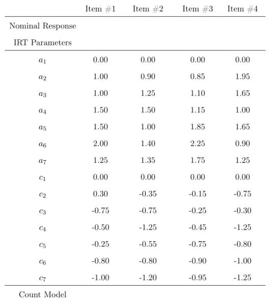
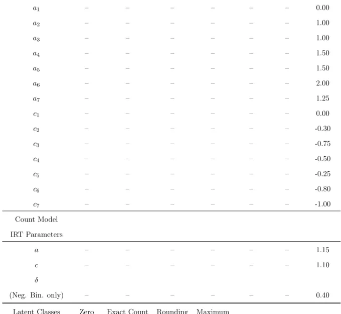
2 Simulation parameters for the full latent class IRT model, N = 10,000 . . . 33
3 Simulation parameters for the full latent class IRT model, N = 10,000 . . . 40
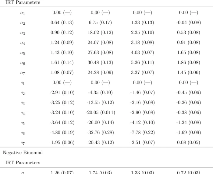
4 Parameter estimates from the negative binomial latent class IRT model fit to the
BRFSS data , N = 10,000 . . . 49
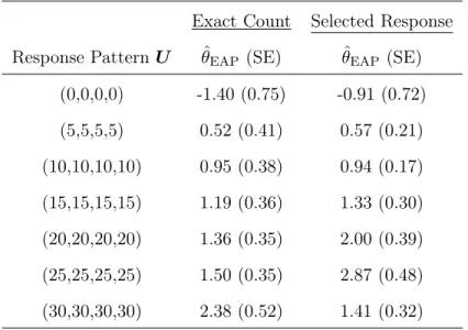
5 Expected scale scores and posterior standard deviations for different response
pat-terns: The exact count class vs. the rounding/selected response class. . . 63
6 AIC and BIC values for competing latent class IRT models; the best-fitting values
are shown in bold. . . 67
7 Parameter estimates for the latent class IRT model with a Poisson IRT model for
the exact count class fit to BRFSS data, N = 10,000. . . 73
8 Frequencies of observed vs. expected responses to “How many days did a mental
health condition or emotional problem keep you from doing your work or other usual activities?” according to latent class IRT model with a Poisson component for the
exact count class and a nominal component for the rounding/selected response class. 76
9 Parameter estimates for the latent class IRT model with a negative binomial IRT
model for the exact count class fit to BRFSS data,N = 10,000. . . 77
List of Figures
1 Frequency histograms for four general emotional health items from the BRFSS (2014)
eliciting count responses. . . 4
2 Frequency histograms for the emotional health subscale from the BRFSS (2012)
comprising six Likert-type items and one count item. . . 21
3 Tree diagram of full latent class IRT model . . . 25
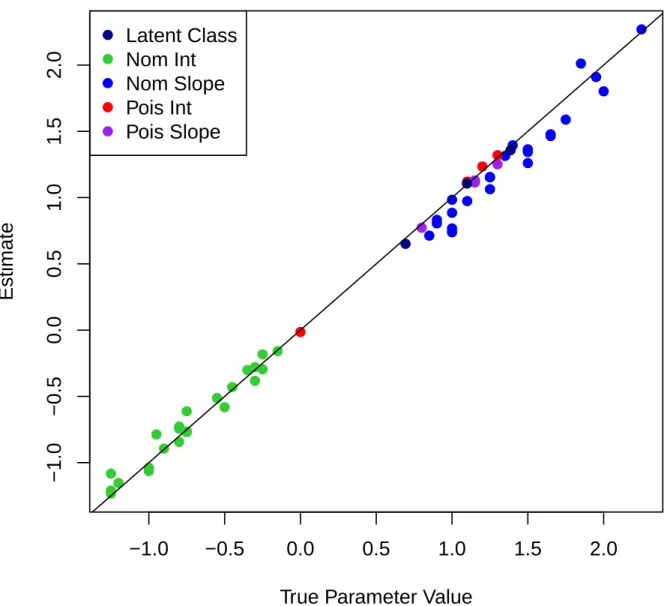
4 Latent class IRT model with a Poisson IRT model for exact count class and a nominal
response IRT model for rounding/selected response class: Estimated parameters vs.
data-generating parameters, for data simulated using the parameters in Table 2. . . . 44
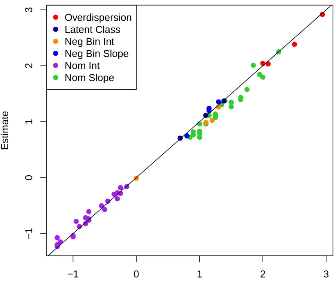
5 Latent class IRT model with a negative binomial IRT model for exact count class
and a nominal response IRT model for rounding/selected response class: Estimated parameters vs. data-generating parameters, for data simulated using the parameters
in Table 2. . . 46
6 Empirical response distributions vs. response distributions simulated from the
esti-mated model parameters in Table 4. . . 50
7 NRM item parameter estimates as a function of response category within the
round-ing/selected response class. . . 52
8 NRM trace lines for the rounding/selected response class. . . 54
9 Negative binomial model trace lines for the exact count class. . . 56
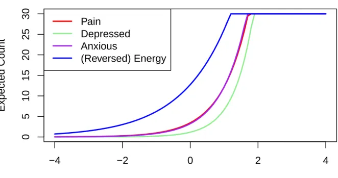
10 Expected counts as a function of the latent variable for members of the exact count
class. . . 58
11 IRT scale scores (response pattern EAPs) for members of the exact count and
round-ing/selected response classes. . . 61
12 Scatterplot of scale scores computed for the same persons from negative bimomial
model trace lines (x-axis) vs. NRM trace lines (y-axis). . . 64
13 Posterior standard deviations (SEs) as function of scale scores. . . 65
14 Latent class IRT model with a Poisson IRT model for the exact count class and a
nominal response IRT model for the rounding/selected response class: Estimated parameters vs. data-generating parameters, for data simulated using the parameters
in Table 3. . . 69
15 Latent class IRT model with a negative binomial IRT model for the exact count
class and a nominal response IRT model for the rounding/selected response class: Estimated parameters vs. data-generating parameters, for data simulated using the
parameters in Table 3. . . 71
16 Empirical response distributions vs. response distributions simulated from estimated
17 GRM trace lines for the six Likert items on the BRFSS mixed item-type scale. . . . 79
18 Poisson (upper) and NRM (lower) trace lines for the count item on the BRFSS mixed
item-type scale. . . 81
19 Precision of measurement as a function of scale scores that are computed with and
Chapter 1: Background and Motivation
Count data are prevalent in the social sciences. In psychology, for example, a researcher may
be interested in predicting the number of occurrences of a specific behavior based on a set of
covariates, such as using scores on an attachment scale to predict the number of perpetrations
of unwanted pursuit behavior in broken up couples (e.g., Loeys, Moerkerke, De Smet, & Buysse,
2012). Statistical methods for the analysis of univariate count outcomes have existed for several
decades and are commonly variants of the log-linear model, including Poisson regression (e.g.,
Agresti, 2002; Cameron & Trivedi, 2013; McCullagh & Nelder, 1989), negative binomial
regres-sion (e.g., Hilbe, 2011), and their zero-inflated extenregres-sions (e.g., Lambert, 1992). These models
have widespread application in fields such as psychology (number of drinks consumed per week,
Lewis, Neighbors, Geisner, Lee, Kilmer, & Atkins, 2010), medicine (number of tumors at time
of death, Dunson & Herring, 2005; number of sexual partners, Roberts & Brewer, 2008) and
economics (number of hospital stays, Deb & Trivedi, 1997), among others. Loeys et al. (2012)
recently published a review of some of the current challenges and proposed solutions to modeling
univariate count outcomes in psychological research.
Psychological questionnaires that comprise multiple items eliciting count responses are
be-coming increasingly common, particularly in the domain of public health. Often, these surveys
are designed to assess the severity of symptoms and ask respondents to recall the frequency of
various thoughts or behaviors over a pre-specified period of time. For example, a survey that
is intended to measure depression may include an item asking the respondent to estimate the
number of days he or she has felt sad in the past month; a survey measuring alcohol dependence
may ask the respondent to report the number of drinks he or she consumes during a typical
week. As an indication of the prevalence of these types of items in survey research, Table 1 lists
some examples of published questionnaires including at least one count item.
While statistical methods for the analysis of a single count outcome are widely available (e.g.,
Questionnaire Source/Authors
Behavioral Risk Factor Surveillance System Centers for Disease Control (1984-present)
National Health and Nutrution Examination Survey Centers for Disease Control (1971-present)
Youth Risk Behavior Survey Centers for Disease Control (1991-present)
WHO Disability Assessment Schedule 2.0 World Health Organization (1998-present)
HIV Risk-Taking Behaviour Scale Ward, Darke, & Hall (1990)
Cognitive Appraisal of Risky Events Scale Fromme, Katz, & Rivet (1997); Katz, Fromme, & D’Amico (2000)
Inventory of Statements about Self-Injury Klonsky & Glenn (2008)
Self-Injurious Thoughts and Behaviors Interview Nock, Holmberg, Photos, & Michel (2007)
Table 1. Questionnaires with at least one item eliciting a count response
multivariate count outcomes, such as responses to sets of count items on questionnaires, are
considerably less well-developed. A question that arises from the content of these questionnaires
is how one can derive meaningful scores from count responses that reflect the construct that
is of interest (e.g., depression or alcohol dependence). Item response theory (IRT), rooted
in educational measurement (Thissen & Wainer, 2001), has played an increasing role in the
assessment of psychiatric and health outcomes (e.g., Finch & Pierson, 2011; Finkelman, Green,
Gruber, & Zaslavsky, 2011; Sawatzky, Ratner, Kopec, & Zumbo, 2012; Wall, Park, & Moustaki,
2015). Educational applications of IRT have direct analogs in psychiatric assessment (Reise
& Waller, 2009) – just as a latent ability level is thought to underlie a person’s answers to
items on an educational test, a latent variable is also believed to influence someone’s responses
to items on a questionnaire assessing health status. For example, someone with a high level
of depression is likely to endorse the more severe response categories on items comprising a
depressive symptoms scale, just as someone with high proficiency is expected to select correct
responses on an educational test.
The IRT literature is heavily focused on the analysis of binary, ordinal, and nominal item
types, likely due to IRT having its origins in educational assessment – one is unlikely to find a
count item on a math or reading test. A reasonable approach to modeling multivariate count
responses might be to modify traditional IRT techniques, invoking a log link function in place
of the usual logit or probit link and a Poisson distribution in place of a Bernoulli or multinomial
conditional response distribution. However, if one examines most count data more closely, a
To illustrate the analytic issues, Figure 1 shows histograms of 5,000 randomly selected
re-sponses to four items about general health found on the Behavioral Risk Factor Surveillance
System (BRFSS; CDC, 1984-present). Each item asks respondents to report the number of days
in the past 30 days they have experienced a specific symptom, thought, or behavior. It is clear
from the histograms that the observed responses do not follow a standard count distribution
(e.g., Poisson, negative binomial). Not only is there a very large proportion of respondents
reporting zero days, much larger than would be expected from a standard count distribution,
but there is also a substantial proportion of respondents reporting the maximum of 30 days.
Inflation at zero and the maximum may reflect unique subsets of people with either a complete
absence or such a severe presence of depression that these respondents do not come from the
same populations as the rest of the sample. Further, there is noticeable inflation at days that
are multiples of five. For example, it is more common for people to report feeling depressed for
five days than four or six days, even though these adjacent values are in theory no less plausible.
This type of inflation at preferred digits is commonly referred to as heaping or data coarsening
in the biostatistics literature (Heitjan & Rubin, 1990; H. Wang & Heitjan, 2008; Wright & Bray,
2003). Simply modifying a traditional IRT model to invoke a log link function and a Poisson
conditional response distribution is not likely to account for the potential subpopulations and
individual differences that result in the histograms observed in Figure 1. This research attempts
to address this problem by combining methodological approaches from three related but
dis-tinct literatures: IRT models for multivariate count data, latent variable models for heaping
and extreme responding, and mixture IRT models.
1. Item Response Models for Multivariate Count Data
Over the past decade, the literature on psychometric models for multivariate count data
has grown (Bockenholt, Kamakura, & Wedel, 2003; L. Wang, 2010; Wedel, Bockenholt, &
Ka-makura, 2003); however, it remains quite sparse, especially in comparison with the advancement
seen in other areas of IRT. Most recently, L. Wang (2010) developed an item response model for
zero-inflated Poisson data (IRT-ZIP) using a non-linear mixed modeling framework. Based on
Lambert’s (1992) original zero-inflated Poisson regression model, Wang’s model is a latent
vari-able mixture model that accounts for two different response processes: the zero process, which
During the past 30 days, for about how many days did pain make it hard for you to do your usual
activities, such as self−care, work, or recreation?
Number of Days
Frequency
0 5 10 15 20 25 30
0
1000
2000
3000
4000
5000
6000
During the past 30 days, for about how many days have you felt sad, blue, or depressed?
Number of Days
Frequency
0 5 10 15 20 25 30
0
1000
2000
3000
4000
5000
6000
During the past 30 days, for about how many days have you felt worried, tense, or anxious?
Number of Days
Frequency
0 5 10 15 20 25 30
0
1000
2000
3000
4000
During the past 30 days, for about how many days have you felt very healthy and full of energy?
Number of Days
Frequency
0 5 10 15 20 25 30
0
500
1000
1500
2000
2500
3000
relates to the expected event count, given that the event has a chance of occurring. Consider an
item that asks respondents to report the number of alcoholic beverages they have consumed in
the last week. There are at least two reasons someone might register a response of zero. One
rea-son is that the perrea-son may simply not drink alcoholic beverages, being an abstainer, and would
thus respond with zero to any question related to the frequency of alcohol consumption. On
the other hand, someone may report zero not because that person is an abstainer, but because
he or she, either by chance or some other reason, has not consumed any alcoholic beverages
in the last week. While both underlying processes result in the same observed response, these
two types of zeros are qualitatively different. Zero-inflated Poisson models, including Wang’s
IRT-ZIP model, can be used to distinguish probabilistically the abstainers from the people who
normally drink but may not have consumed any alcoholic beverages in the specified time frame.
According to Wang’s IRT-ZIP model, the observed count response Uij for personi on item
j is expressed
Uij ∼
0, with probability1−pij
Poisson(λij), with probabilitypij
(1)
in which
P(Uij = 0) = (1−pij) +pije−λij (2)
P(Uij =uij) =
pije−λijλ uij
ij uij!
, uij = 1,2, ... (3)
The probability pij of person i being in the Poisson process on item j, and λij, the expected
count for personion itemj given that person iis in the Poisson process, can then be modeled
as a function of item parameters (a1j, a2j, b1j, b2j) and a latent variable (θi):
For model identification, θi is assumed to follow a standard normal distribution. There are
two sets of item parameters; one set of parameters is for the Poisson process (Equation 4), while
the other corresponds to the zero state (Equation 5). The parameters a1j and a2j are item
discriminations for the Poisson process and zero state, respectively; the larger these values, the
more discriminating the item is in estimating scores on the latent variable. The parametersb1j
and b2j are the location parameters for the Poisson process and zero state, respectively. The
larger b1j, the more difficult it is for someone in the Poisson process (i.e, someone who is not
an abstainer) with a given latent variable score to reach a high expected count; the larger b2j,
the more likely it is for someone with a given latent variable score to be classified as part of the
zero-state (abstainers) and not enter the Poisson process. By varying the values of these two
sets of parameters, one observes different proportions of zero-inflation and ranges of expected
counts. Wang parameterized the IRT-ZIP model as a generalized multilevel model that can be
estimated using marginal maximum likelihood. The marginal log likelihood for item parameter
sets a andbgiven observed responses uis written
l(a,b|u) = N
X
i=1
log
Z J
Y
j=1
p(uij|a,b, θi)N(θi)dθi, (6)
in whichp(uij|a,b, θi)can be re-expressed based on the conditional probabilities from Equations
2 and 3:
p(uij|a,b, θi) = [(1−pij) +pije−λij]1−yij
"
pije−λijλ uij
ij uij!
#yij
(7)
whereyij = 1 if uij 6= 0 and yij = 0 otherwise.
Wang implemented marginal maximum likelihood in SAS PROC NLMIXED, using adaptive
quadrature to approximate the integral in Equation 6. Treating the estimated item parameters
as fixed, she then computed latent variable scores using empirical Bayes methods. Wang applied
the IRT-ZIP model to data from the National Longitudinal Survey of Youth, combining three
items to form a substance use scale and examining trends in substance use over time.
While Wang’s IRT-ZIP model provides an item response modeling framework for analyzing
Mainly, it assumes that the non-perfect zero state is a Poisson process; however, real world data
analysis suggests that the Poisson distribution rarely describes observed count responses. This
is especially true of retrospective self-report data in which heaping is prevalent (e.g., H. Wang
& Heitjan, 2008), as illustrated in Figure 1. For this reason, a more flexible modeling approach
may be useful.
2. Heaping and Response Style
H. Wang and Heitjan (2008) examined self-reported counts of cigarette use as the outcome
of a clinical trial on smoking cessation. They were interested in evaluating the effect of an
antidepressant on smoking abstinence in a sample of smokers intending to quit. At a follow-up
assessment after being instructed to quit smoking, participants were asked to retrospectively
report the number of cigarettes smoked each day. Frequency distributions of cigarette counts
revealed a very large proportion of zeros, potentially representing a subset of respondents who
had successfully quit smoking, as well as heaped responses at multiples of five. In particular,
the authors noted the unsurprising heaping at 20, corresponding to the number of cigarettes
sold in a package.
To account for the large proportion of respondents reporting zero cigarettes, as well as the
non-trivial heaping at 5, 10, and 20 cigarettes, H. Wang and Heitjan (2008) introduced a model
in which the observed cigarette count was a function of both the unobserved true cigarette count
and a latent “heaping behavior” variable. Their discrete latent heaping behavior variable could
take on one of four values, depending on the type of rounding behavior: exact count, multiple
of 5, multiple of 10, or multiple of 20. They also modeled the potential relationship between the
heaping behavior and the underlying count variable according to a proportional odds model,
hypothesizing that coarser rounding may be associated with larger true cigarette counts. They
used Bayesian methods to estimate model parameters, fitting a series of zero-inflated Poisson
and negative binomial models that either ignored or accounted for heaping, and found strong
evidence for improved model fit after accounting for heaping. They also found that heaping had
a sizable effect on the estimated quit probability and mean cigarette count, with over 40% of
the sample exhibiting some type of rounding behavior.
From a psychometric perspective, Wang and Heitjan’s model could be considered a
cigarette addiction – influence the observed cigarette count, but there is an additional individual
differences variable influencing people’s rounding behavior: Someone at high levels of the latent
variable that reflects rounding is more likely to exhibit coarse rounding behavior. In their model,
Wang and Heitjan treated rounding behavior as discrete with ordered categories, similar to a
latent class variable.
The idea that a self-reported cigarette count is influenced by an underlying variable is not
unlike psychometric models, which assume that a latent variable underlies observed responses
to questionnaire items; however, Wang and Heitjan’s model dealt only with a single count
out-come, not the multiple items or measures that are routinely used in psychometric modeling.
Other statisticians have also developed models for heaping in univariate outcomes. For
ex-ample, Heitjan and Rubin (1990) used multiple imputation to model rounding in self-reported
age, treating the estimation of true age as a missing data problem. Ridout and Morgan (1991)
introduced a model to account for heaping in women’s retrospective reports of the number of
menstrual cycles before a positive pregnancy, with digit preference often occurring at 6, 12,
and 3 cycles. Wright and Bray (2003) used Bayesian mixture modeling techniques to capture
the rounding process in clinician-reported measurements from ultrasound images, in which
dif-ferent components of the mixture model represented difdif-ferent levels of rounding. Review of
the biostatistics literature, however, has not uncovered methods of accounting for heaping in
multivariate count outcomes.
While the psychometrics literature does not include specific models for heaping in
multivari-ate count data, research on extreme responding on surveys addresses a similar concept within
an IRT framework. Bolt and Johnson (2009) used a multidimensional nominal response IRT
model to account for the individual differences that increase the probability that some
respon-dents select the “strongly disagree” or “strongly agree” options on a rating scale; this tendency
is referred to as extreme response style (ERS). Research suggests that ERS can interfere with
the response process purportedly being modeled using IRT, and if not accounted for, can result
in less precise estimates of the latent variable of interest, biased item parameter estimates, and
spurious correlations of latent variable estimates with other variables (Bolt & Newton, 2011;
Jin & Wang, 2014; Thissen-Roe & Thissen, 2013). Similar consequences may hold if heaping in
Bolt and Johnson (2009) modeled item responses as a function of both the substantive
construct of interest and an ERS latent variable. According to their model, the probability of
selecting response categoryk on itemj is expressed
P(Uj =k|θ1, θ2, ..., θd) =
exp(ajk1θ1+ajk2θ2+...+ajkdθd+cjk)
PK
h=1exp(ajk1θ1+ajk2θ2+...+ajkdθd+cjk)
, (8)
whereθ1,θ2, ...,θd are thedlatent variables assumed to underlie someone’s category selection,
and aandc are the slope and intercept parameters for categorykon item j. One of the latent
variables may reflect ERS. For example, Bolt and Newton (2011) described a multidimensional
nominal response model in which there is a latent variable related to the construct of interest,
θ1, and a latent variable for ERS,θERS,
P(Uj =k|θ1, θERS) =
exp(ajk1θ1+ajk2θERS+cjk)
PK
h=1exp(ajk1θ1+ajk2θERS+cjk)
. (9)
θERS is identified by a pattern of largeajk2 parameters for extreme responses, and smaller
ajk2 parameters for less extreme responses. These models allow estimation of IRT scores that
reflect each latent variable, with scores accounting for the simultaneous influence of the
sub-stantive construct and response style on the observed responses.
Other researchers have conceptualized item responses as observed outcomes resulting from
a sequence of internal decisions (Böckenholt, 2012; De Boeck & Partchev, 2012; Thissen-Roe &
Thissen, 2013). Böckenholt (2012) and De Boeck and Partchev (2012) proposed a tree structure
for capturing the ways in which individuals may differ in answering test items. They argued
that while IRT models tend to assume a single response process, it is possible that multiple
response processes are at play when someone responds to a questionnaire item. Böckenholt
(2012) provided an example of a Likert-type item with five categories: strongly disagree, disagree,
neither disagree or agree, agree, andstrongly agree. At Process I, the respondent decides whether
he or she expresses an opinion. If not, the person selects neither disagree or agree and the tree
process ends; responses for the remaining processes are coded as missing. If the respondent
chooses to express an opinion, the tree branches to Process II where the respondent decides
the direction of the opinion: agreement vs. disagreement. Either choice results in branching to
or agree if the opinion is positive, strongly disagree or disagree if the opinion is negative. The
probability of a particular response category can be expressed as the product of the respective
branch probabilities. Böckenholt’s (2012) model does not assume that the same latent variable
underlies each process. As noted in Thissen-Roe and Thissen’s (2013) review of the literature,
however, Böckenholt’s (2012) and De Boeck and Partchev’s (2012) tree structure models are
members of the generalized linear mixed model (GLMM) family and cannot handle bilinear
functions; therefore, item discrimination parameters are not included in any of the response
process models. An additional limitation of Böckenholt’s (2012) model is that it does not have
the feature that more than one branching path can lead to the same observed response.
Using an argument similar to Böckenholt’s (2012) and De Boeck and Partchev’s (2012),
Thissen-Roe and Thissen (2013) developed a two-decision model for responses to Likert-type
items. They posited that in responding to each Likert-type item, examinees answer two internal
items. The response to the first pseudo-item is the realization of a binary process: Does the
respondent agree or disagree? The response to the second pseudo-item describes the strength of
the first response: Given that the respondent agrees (or disagrees), how strong is that agreement
(or disagreement)? Like Böckenholt’s (2012) model, the probability of observing a response
category is expressed as the product of the probabilities of the relevant outcome occurring at
each stage. At the first stage, the probability is a function of the latent variable(s) the items
are designed to measure; at the second stage, the probability is a function of the intended latent
variable as well as a different latent variable that reflects the secondary construct of extreme
response behavior. Unlike Böckenholt’s (2012) and De Boeck and Partchev’s (2012) models,
Thissen-Roe and Thissen’s (2013) model is not a member of the GLMM family and thus can
accommodate an item discrimination parameter. The central idea behind these tree structure
models is that response intensity is modeled by a separate response process and with a different
latent variable than response direction.
Biostatistical models for heaping and psychometric models for extreme responding developed
in different fields and from different methodological frameworks; however, both approaches
converge on the idea of a latent variable underlying individual differences in the response process.
The tree structure psychometric models posit that one latent variable underlies the first decision
underlies the second decision about intensity of opinion. A similar approach could be adopted in
modeling zero-inflated count data with heaping. One latent variable may underlie the presence
or absence of the chance of a countable behavior; given that the respondent may potentially
exhibit a non-zero frequency, a second latent variable could reflect the intensity of the frequency
and a third latent variable could represent individual differences in response style (RS) – or in the
case of count data, rounding behavior. Some extreme response models treat RS as a continuous
latent variable (e.g., Böckenholt, 2012; Bolt & Johnson, 2009; Bolt & Newton, 2011; De Boeck
& Partchev, 2012; Thissen-Roe & Thissen, 2013); accordingly, differences in scores on the latent
construct represent quantitative differences in response styles. Other models assume that RS is
a discrete latent variable, in which categorical latent classes correspond to qualitatively different
types of response styles (e.g., Maij-de Meij, Kelderman, & van der Flier, 2008; Moors, 2008;
Rost, Cartensen, & Von Davier, 1997). The latter is more similar to the approach taken by
biostatisticians including H. Wang and Heitjan (2008), who group people into rounding classes
depending on their response style. In addition to accounting for distinct response styles, latent
class IRT, commonly referred to as mixture IRT, has potential application to the analysis of
multivariate count data.
3. Mixture Item Response Theory
Unlike traditional item response models, mixture item response models assume that the
observed responses are sampled from a population that has a number of subgroups or
subpop-ulations (Rost, 1990, 1997; von Davier & Rost, 2006). Item parameters or even the parametric
form of the item response model may vary across these subgroups. Under the assumption of local
independence, the marginal mixture distribution of the observed item responsesu= (u1, ..., uJ)
is expressed
p(u1, ..., uJ) = G
X
g=1
π(g)
Z
θ
Y
j
pgj(uj|θ)φ(θ|g)dθ
(10)
where RθQ
jpgi(uj|θ)φ(θ|g)dθ is the conditional probability of response pattern (u1, ..., uJ) in
subpopulation g, written p(u1, ..., uJ|g). Observed responses and latent variable densities are
conditional on the subpopulation, withπ(g)denoting the proportion of the population belonging
unobserved variables and are estimated as part of the model.
von Davier and Rost (2006) reviewed applications of mixture item response modeling to
educational measurement; for example, student strategy usage on an educational test can be
treated as an unobserved latent class variable. Depending on the strategy used, items may vary
in their difficulty parameters, with different test taking strategies making certain items easier
to answer correctly (Bolt, Cohen, & Wollack, 2001; Mislevy & Verhelst, 1990; Rost, 1990).
Other researchers have used mixture item response modeling to account for test speededness
(Bolt, Cohen, & Wollack, 2002; Yamamoto & Everson, 1997). Such models often include a
“speeded” class comprising individuals who had insufficient time to answer items at the end of
a test, and a “nonspeeded” class comprising the individuals who had enough time to answer
all items; potential qualitative differences in response processes are accounted for in mixture
item response models. The same rationale can be applied to mixture item response modeling in
health outcomes research (Finch & Pierson, 2011; Finkelman et al., 2011; Muthen & Asparouhov,
2006; Sawatzky et al., 2012). Respondents belonging to different latent classes – for example,
a subgroup of people who abstain from drinking but are nonetheless asked a series of questions
relating to symptoms of alcohol dependence – may not engage with the items in the same way
as other subgroups in the population.
Finkelman et al. (2011) proposed a mixture IRT model for binary zero- and K-inflated
health questionnaire data. They addressed the measurement of psychiatric disorders with low
prevalence, arguing that the normal prior commonly used as the population distribution in IRT
is unrealistic when people with high levels of the latent variable are rare. When many of the
respondents in the population possess none or very low levels of the construct being measured,
such as a large group of people not endorsing any of the criteria on a symptoms checklist, it is
plausible that the latent variable follows a mixture distribution with a zero-inflated component.
In the psychometrics literature, these types of clinical constructs are sometimes referred to as
“unipolar” because it is possible for a respondent to exhibit a complete absence of the latent
variable (Reise & Waller, 2009; Wall et al., 2015). Sometimes in clinical assessment, there
may also be a small subset of respondents who are extreme at the other end of the latent
variable, endorsing all possible symptoms on a checklist. Finkelman et al. (2011) referred to the
the challenges associated with measuring low-prevalence psychiatric disorders, Finkelman et al.
(2011) used a latent class item response model to account for extreme subpopulations. One latent
class describes the people with no symptoms (the no-symptom group); a second class describes
the people exhibiting most or all of the symptoms (the all-symptom group). The remaining
latent class, labeled the graded class, describes people along the severity continuum implied
by a traditional item response model with a normal prior. It is the presence of respondents
from potentially different populations that requires mixture IRT in place of a conventional IRT
model.
For a general latent class IRT model, the probability of person i endorsing itemj is given
by
Pj = G
X
g=1
πgPgj. (11)
In Equation 11, class membership is indexedg= 1, ..., Gand Pgj is the conditional probability
of someone in classg endorsing item j. Finkelman et al. (2011) used indicator variables I1,I2,
and I3 to denote membership in the no-symptom class, the graded class, and the all-symptom
class, respectively;π1,π2, andπ3 = 1−π1−π2 are the proportions of people in the population
belonging to the respective classes. The probability of endorsing item j is 0 if I1 = 1 and 1 if
I3 = 1. IfI2 = 1, the probability of endorsing itemj is given by the 2-parameter logistic (2PL)
IRT model
Pj(Uj = 1|θi) =
exp{aj(θi−bj)} 1 + exp{aj(θi−bj)}
(12)
in whichaj is the discrimination parameters for itemj,bj is the difficulty parameter for itemj,
andθi is the latent variable for personi. For this graded class, a standard normal prior is used
as is conventional in IRT. Because someone in the no-symptom class will never endorse the item,
and someone in the all-symptom class will always endorse the item, these two classes have item
response models that are degenerate, with Pgj = 0 for the no-symptom class and Pgj = 1 for
the all-symptom class. Finkelman et al. (2011) used an EM algorithm to estimate IRT model
parameters and proportions of respondents in each class. Because the authors used a nationally
with survey weights.
They let u = (u1, ..., uJ) be a vector of 0s and 1s representing the response pattern for
an individual, with 0 = (0, ...,0)and 1 = (1, ...,1) denoting the response patterns for the
no-symptom class and all-no-symptom class, respectively. They let Nu be the sum of the weights
of individuals with response pattern u, with special cases N0 and N1 for individuals with no
symptoms and all symptoms, respectively. For a set of item parametersα, the log likelihood is
expressed
l(α, π0, π1, π2;{ui}I1) =N0log[π0+π2P(U = 0|α, φ(θ), I2 = 1)]
+N1log[π1+π2P(U = 1|α, φ(θ), I2 = 1)]
+ X
u∈{0/ ,1}
Nulog[π2P(U =u|α, φ(θ), I2= 1)]
(13)
in which P(U = u|α, φ(θ), I2 = 1) is the probability of observing response pattern u for
someone in the graded component of the model. Like zero-inflated count data, a main issue
with this type of data is that the people with response pattern0 and in the no-symptom class
are indistinguishable from those with response pattern 0 who are in the graded class, and the
people with response pattern 1 and in the all-symptom class are indistinguishable from those
with response pattern 1 who are in the graded class. That is, the total weights of graded
component individuals satisfying u=0 and u=1 are treated as missing data. The observed
data are the weights and response patterns of all individuals satisfyingu∈ {/ 0,1}(and therefore
in the graded component). Finkelman et al. (2011) used an EM algorithm in Mplus to estimate
the IRT parameters and proportions of people in each class. They demonstrated an empirical
example using data from the oppositional defiant disorder (ODD) and conduct disorder (CD)
symptom scales of the US National Comorbidity Survey Adolescent supplement. As expected,
the two-class and three-class mixture IRT models fit the data better than a unidimensional 2PL
model, suggesting subsets of respondents with extreme levels of the latent variable who are not
well described by the same model as the general population.
More recently, Wall et al. (2015) proposed a similar model for measuring psychiatric disorder
each symptom on a clinical checklist of alcohol dependence as a binary item, with endorsement
of the item/symptom suggesting higher levels of the latent variable. As is common in clinical
assessment, a large proportion of their sample did not endorse any of the symptoms, potentially
representing a fundamentally different subset of individuals from those the assessment was
de-signed to measure; therefore, instead of assuming normality of the latent variable, the authors
used a composite population distribution composed of a mixture of normals, with a degenerate
component for the subgroup of respondents who did not endorse any of the symptoms. They
considered the population to comprise G subgroups, each coming from a normal distribution
with meanµgand varianceσg2, mixed in proportion to the group sizes,η1,η2,...,ηG; for the
peo-ple endorsing none of the symptoms, they assumed a degenerate distribution. Like Finkelman
et al. (2011), they used a 2PL IRT model to describe the non-degenerate class, using
maxi-mum likelihood with an EM algorithm in Mplus to estimate model parameters. Results of their
simulation study suggested that the assumption of a normal latent variable distribution in the
presence of a non-pathological subset of respondents leads to biased item parameter estimates
and shrunken IRT scores that provide less separation of individuals.
Mixture IRT can also be conceptualized as testing for differential item functioning (DIF)
when the groups are unknown (Cohen & Bolt, 2005; Samuelson, 2008; von Davier & Rost, 2006).
Finch and Pierson (2011) used mixture IRT to analyze items on the Youth Risk Behavior Survey
(YRBS). They were interested in identifying subgroups of adolescents most at risk for engaging
in risky behaviors based on observed response patterns, allowing for potential differences in item
parameters depending on latent class membership. Specifically, they examined whether certain
items were more or less discriminating or easily endorsed across different at-risk subgroups in the
population. Their model was based on the 2PL IRT model with group-specific item parameters
and level of the latent variable,
Pj(Uj = 1|g, θg) =
exp{ajg(θg−bjg)} 1 + exp{ajg(θg−bjg)}
. (14)
Each respondent is assigned to a latent class as part of model estimation, and the proportion
of respondents belonging to each class (πg) is estimated under the constraintPGg=1πg = 1. The
in risky behaviors, such that endorsement of the item suggested greater propensity for risk
taking behavior; it is worth nothing, however, that not all items were originally binary. For
example, the item “How many times have you smoked marijuana in the previous month” was
recoded from its original binned count response to a binary response. While item format was
not central to the authors’ research goals, it is important to point out that the practice of
dichotomizing count responses does occur in psychological research, and while it reduces analytic
burden, the loss of information may have unintended consequences. Understanding the potential
effects of binning or dichotomizing count data is one of the motivating factors for the current
research. Finch and Pierson (2011) found that a four-class mixture IRT solution fit the data
best, and that certain items were more discriminating or easily endorsed depending on the
latent class. For example, they identified a latent class with an especially high propensity
of engaging in risky sexual activities; for this particular class, the items pertaining to sexual
behavior were not as discriminating as items relating to other risky behaviors. The authors
noted the potential usefulness of mixture IRT modeling in clinical assessment, with
group-specific parameters allowing mental health professionals to focus on items and behaviors that
are most discriminating in identifying the highest-risk adolescents within specific subgroups of
risk-takers.
Sawatzky et al. (2012) applied a similar mixture IRT model to the measurement of patient
reported outcomes. Like Finch and Pierson (2011), they were interested in fitting an item
response model to data from a potentially heterogeneous population. Their model was based on
the graded response model (GRM), in which the probability of responding at or above category
kon item j is expressed
Pjk(Uj ≥k|θ) =
exp{aj(θ−bjk)} 1 + exp{aj(θ−bjk)}
(15)
wherebjk is the threshold between the categories of itemj andai is the discrimination
param-eter for item j. To account for potential population heterogeneity, the authors introduced an
additional subscript,g, for group membership:
Pjkg(Uj ≥k|θ, G=g) =
exp{ajg(θ−bjkg)} 1 + exp{ajg(θ−bjkg)}
G is the latent class variable withg classes, and f(x) =PG
g=1πgfg(u), wheref is the mixture
of latent class-specific distributions andπk is the proportion of respondents in each class, with
PG
g=1πg = 1. This model is very similar to that of Finch and Pierson (2011), only with the
GRM used in place of the 2PL model. The authors used maximum likelihood via an EM
algorithm to estimate model parameters. As an empirical example, they analyzed the physical
functioning subscale of the SF-36 Health Survey, consisting of 10 items designed to measure
the general health status of the US population. Each item asked the respondent to report the
degree to which his or her health limits daily activities; response options are “Yes, limited a lot”,
“Yes, limited a little”, or “No, not limited at all”. One might hypothesize that the population of
interest comprises qualitatively different subgroups. For example, in the general population there
is possibly a group of people who experience no physical functioning impairment; this group may
interpret the items differently from the rest of the population, making the scale less appropriate
for samples from that population. Sawatzky et al. (2012) used mixture IRT to answer this
question empirically and arrived at a three-class solution, suggesting a class of people with
very few physical limitations and two classes of people with more severe physical functioning
limitations. The second class reported less struggle with more routine physical functioning
activities such as climbing stairs and walking a block, whereas the third class reported struggle
with both routine and more challenging activities. Mixture IRT highlights those items that may
be best suited for the assessment of subgroups within clinical populations.
4. Research Questions
A review of the literature suggests three methodological approaches for solving three distinct
problems in measurement: Poisson and zero-inflated Poisson psychometric models for the
anal-ysis of multivariate zero-inflated count data (L. Wang, 2010); latent variable models to account
for heaping and response style, including heaping in univariate count outcomes (e.g., H. Wang
& Heitjan, 2008) and extreme responding in multivariate item response data (e.g., Böckenholt,
2012; Bolt & Johnson, 2009; Bolt & Newton, 2011; De Boeck & Partchev, 2012; Moors, 2008;
Thissen-Roe & Thissen, 2013); and mixture IRT models for clinical assessment in potentially
heterogeneous populations (Finch & Pierson, 2011; Finkelman et al., 2011; Sawatzky et al.,
2012; Wall et al., 2015).
studies that provide an item response modeling framework for multivariate count outcomes that
also accounts for zero-inflation, inflation at the maximum (K-inflation), and heaping. Finkelman
et al.’s (2011) mixture IRT model accounts for inflation due to large proportions of respondents
with a complete absence or very severe presence of the latent variable, but their model includes
only binary items that comprise a checklist of symptoms. The same limitation applies to Wall
et al.’s (2015) mixture IRT model for zero-inflation in the measurement of psychiatric disorders
and Finch and Pierson’s (2011) mixture IRT model for the analysis of risky youth behavior.
Sawatzky et al.’s (2012) mixture IRT model is slightly more flexible, incorporating ordinal
rating-scale items into the analysis of patient reported outcomes across distinct classes, but
their model still includes only traditional item types that are well suited for conventional IRT
models. A more flexible modeling approach that incorporates complex item types – particularly
those eliciting inflated count responses – is still needed. Wang’s (2010) IRT-ZIP model partially
addresses this need, but her model ignores the issue of heaping at preferred digits. Statisticians
have developed methods to account for heaping in univariate count data (e.g., H. Wang &
Heitjan, 2008), but these models tend to consider only a single count outcome; conversely, the
extreme response literature in IRT addresses response behavior in multivariate data but does
not consider count responses (e.g., Böckenholt, 2012; Bolt & Johnson, 2009; Bolt & Newton,
2011; De Boeck & Partchev, 2012; Thissen-Roe & Thissen, 2013). The goal of this research
is to borrow elements from all three existing methodological approaches in developing a latent
class IRT model for multivariate zero-inflated count data that are sampled from a potentially
heterogeneous population. The purpose of including latent classes is not only to account for
inflation at zero and the maximum, but also to account for differences in response style due to
digit or “nice number” preference.
4.1 Primary Aim #1: Addressing Inflation and Heaping in Count IRT Models
In incorporating count items into questionnaires, what are some parsimonious ways to
ac-count for zero-inflation, K-inflation, and heaping? This can be viewed as a latent class IRT
problem, in which latent classes may reveal subpopulations of respondents. Specifically, one
latent class for zero-inflation may represent people who are at a floor level of the latent variable,
or people to whom the questions do not apply. Another latent class may represent those who
to account for individual differences in “nice number” preferences on open-ended count scales,
such as the propensity to select responses that are multiples of five. Depending on the latent
class, a different IRT model can be used to describe the conditional probability of a count
re-sponse. The motivating data for Primary Aim #1 are responses to the four count items from
the BRFSS that form an emotional health subscale, as shown in Figure 1.
Scoring Because clinicians are often interested in scoring individuals on psychological
assess-ments, an additional goal of Primary Aim #1 is to compute IRT scores for people based on
their observed responses to the four count items. For this example, the IRT scores, which are
computed from IRT models that depend on both a latent variable and a latent class
member-ship, represent an emotional health latent variable, where higher scores suggest worse emotional
health. The goal of this aim is to compute IRT scores from the latent class IRT model and
examine different options for reporting scores at the individual-level.
4.2 Primary Aim #2: Are Complex Models Really Needed?
A pragmatic follow-up question to that posed in Primary Aim #1 is whether such complex
modeling techniques are needed, or whether more parsimonious models that omit any of the
latent classes describe the data just as well. The latent class IRT model that accounts for zero
inflation, maximum inflation, and individual differences in response style is the most complex
model, comprising four distinct latent classes; however, simpler models can be obtained by fixing
to 0 different components of the log likelihood of that most complex model. For example, is it
necessary to account for heaping at multiples of five, or will a model that does not account for
heaping describe the data just as well?
4.3 Secondary Aim: What is the value added of including count items on scales?
There is evidence that researchers use open-ended count items on scales, but do these items
provide information above and beyond more conventional response formats? Specifically, do
open-ended count items contribute to measurement precision? This question is motivated by
a specific set of item responses from the BRFSS, shown in Figure 2. The first six items are
traditional Likert-type items that can take on any of five response categories; the last item is a
count item ranging from 0 to 30 and exhibits the same inflation and heaping properties as the
items described in Primary Aim #1. To what extent does including the count item increase
Ho
w often during the past 30 da
ys
did y
ou f
eel ner
v
ous?
None of the time A little of the time Some of the time Most of the time All of the time
0 10000 20000 30000 40000
Ho
w often during the past 30 da
ys
did y
ou f
eel hopeless?
None of the time A little of the time Some of the time Most of the time All of the time
0 10000 20000 30000 40000 50000 60000 70000
Ho
w often during the past 30 da
ys
did y
ou f
eel restless?
None of the time A little of the time Some of the time Most of the time All of the time
0 10000 20000 30000 40000 50000
Ho
w often during the past 30 da
ys
did y
ou f
eel depressed?
None of the time A little of the time Some of the time Most of the time All of the time
0 20000
40000 60000 80000
Ho
w often during the past 30 da
ys did
y
ou f
eel e
ver
ything was an eff
or
t?
None of the time A little of the time Some of the time Most of the time All of the time
0 10000 20000 30000 40000 50000 60000
Ho
w often during the past 30 da
ys
did y
ou f
eel w
or
thless?
None of the time A little of the time Some of the time Most of the time All of the time
0 20000
40000 60000 80000
Ho
w man
y da
ys did a mental health condition
or emotional pr
ob
lem keep y
ou fr
om doing
y
our w
ork or other usual activities?
Number of Da
ys
Frequency
0
5
10
15
20
25
30
0 20000 40000 60000 80000
Figure
2.
F
requency
histo
grams
for
the
emot
ional
health
subscale
from
the
BRFSS
(20
12)
comprising
six
Lik
ert-t
yp
e
items
and
one
coun
t
Chapter 2: Method
1. Primary Aim #1: Addressing Inflation and Heaping in Multivariate Count
Data
The motivating data set for Primary Aim #1 comprises responses to the four items from
the BRFSS (2014) shown in Figure 1 in the previous chapter; these four items are thought to
measure a general emotional health construct, in which higher observed counts indicate worse
emotional health. As described in Chapter 1, there are several analytic challenges present in
these data. Most notably, there is substantial inflation at 0 days, moderate inflation at 30 days,
and heaping at days that are multiples of five. I hypothesized that the inflated proportions of
respondents at these values can be accounted for with latent classes, where each latent class is
characterized by a different IRT model.
First, I present the most general latent class model – this model applies to any set of item
response data. Then, I describe the hypothesized latent classes that are specific to the item
response data in Figure 1. Once the latent classes are defined, the class-specific conditional
probabilities of a count responseuj can be modeled by specifying IRT models that are
appropri-ate for the specific type of response (e.g., a nominal response model for multinomial responses,
a graded response model for ordinal responses, etc.). For simplicity, subscript notation i for
individuals is dropped; only subscriptsj for item and g for latent class are included.
1.1 A Latent Class Model
According to the general latent class model, the unconditional probability of observed
re-sponseuj to itemj can be expressed
Pj = G
X
g=1
πgPgj(Uj =uj), (17)
in whichg denotes latent class membership, πg specifies the probability of belonging to latent
classg, andPgj(Uj =uj) is the conditional probability of observing responseuj from someone
proportions of members in each latent class must sum to one, PG
g=1πg= 1. This is the general
form of a latent class model: Pgj(Uj =uj)can be any type of probability function (IRT model),
and the model can be applied to any set of item response data. In the sections that follow, I
propose specific latent classes based on the BRFSS data in Figure 1.
Defining the Latent Classes To model the item response data shown in Figure 1, I propose
four mutually exclusive latent classes. One latent class describes some, perhaps many, of the
people who respond 0 days to all four items, thus having response vector U =0 = (0,0,0,0).
This class may represent people who are at a floor level of the latent variable, or it may represent
a subset of individuals for whom the items do not apply. An important distinction is that
these people are qualitatively different from those who are not at the floor level of the latent
variable but still exhibit a response vector of zeros, such as an individual who has some degree
of depression but did not experience any symptoms in the past month. Similarly, a second
latent class describes some, perhaps many, of the people who respond 30 days to all four items;
these respondents have a response vector U = 30 = (30,30,30,30). These two latent classes
correspond to response vectors 0 and 30 and will be referred to as the zero class and the
maximum class, respectively. The item response models for these two classes are degenerate:
People belonging to the zero latent class respond 0 to every item with a probability of 1, and
people belonging to the maximum latent class respond 30 to every item with a probability of 1.
In addition to the zero and maximum classes, I propose two graded latent classes that
describe the people falling along the continuum of the latent variable. The first of the graded
classes, which I refer to as the exact count class, comprises the subset of people whose responses
follow a standard count distribution. These are the people who are at some level of the latent
variable and respond to the item as intended; that is, they report the exact number of days
they experienced each symptom in the last month, regardless of whether those numbers are
multiples of five. To model the conditional probability of count response uj from members of
the exact count latent class, a Poisson or negative binomial IRT model can be used; reasons
for choosing each type of count model are explicated in later sections. The other graded class,
which I refer to as the rounding/selected response class, represents the subset of respondents
to the rounding/selected response class may have a true count of 9 days but an observed count
of 10 days. Instead of responding to the item as intended – as an exact count taking on any
of 31 non-negative integers – these individuals may treat the item as multiple choice with only
seven response categories, {0,5,10,15,20,25,30}, or they may round their true count to the
nearest multiple of five. Because respondents belonging to the rounding/selected response class
do not interact with the item as a true count, the Poisson and negative binomial IRT models
are not likely to accurately describe the item response function for this class. Instead, a nominal
response IRT model, designed for multinomial item response data, may be more appropriate.
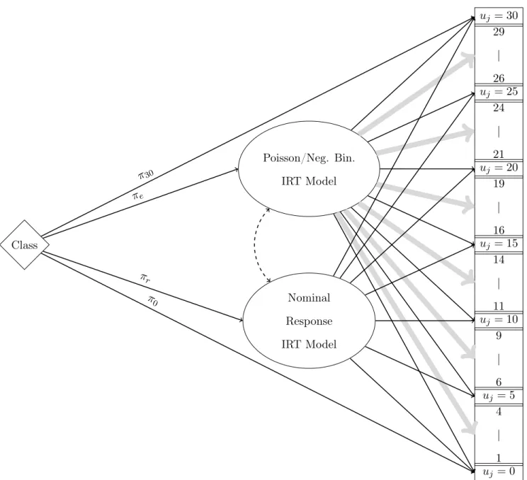
Figure 3 shows a diagram of the proposed latent response processes that result in each of the
31 possible observed counts. According to the model, there are three internal response processes
that can manifest as a zero count. One possibility is that the respondent is a member of the
zero class and thus selects 0 days for every item,U =0= (0,0,0,0); this option is represented
by the direct path from the item to a zero response, without passing through either of the
two IRT models. A second possibility is that the person is part of the exact count class and
happens to report 0 days; that is, the respondent is at some level of the latent variable but has
not experienced any symptoms in the past 30 days. This option is represented by one indirect
path from the item to the zero response: The respondent enters the count IRT model, and it
is through this IRT model that a response of zero is observed. A third possibility is that the
respondent is a member of the rounding/selected response class and reports 0 days; these are
people who are inclined to report days that are multiples of five. Instead of passing through the
count IRT model, these individuals arrive at zero via the nominal response IRT model. Similar
to the three distinct response processes that manifest as a zero count, there are three distinct
response processes that result in an observed count of 30 days. These response processes are
analogous to those described for the zero case and are shown in Figure 3.
Figure 3 shows that for the subset of people belonging to one of the two graded classes, fewer
response processes are possible. Only two distinct paths lead to observed responses that are
non-zero and non-30 multiples of five. The response may be from someone in the exact count class
and thus represent a count that is a realization of a Poisson or negative binomial random variable.
On the other hand, the response may belong to someone in the rounding/selected response class.
Class
Poisson/Neg. Bin.
IRT Model
Nominal
Response
IRT Model
uj = 30 29
| 26
uj = 25 24
| 21
uj = 20 19
| 16
uj = 15 14
| 11
uj = 10 9
| 6
uj = 5 4
| 1
uj = 0 π0
π30
πe
πr
Figure 3. Tree diagram of full latent class IRT model
a count random variable; rather, it is a realization of a multinomial random variable with seven
response categories. Both the Poisson/negative binomial and nominal response IRT models
may yield the same manifest count; however, it is through different response processes that this
multiple-of-five count is reported. The remaining responses that have not been addressed are
the exact counts that are not multiples of five. The only path to these exact counts is via the
Poisson/negative binomial IRT model; people with responses that are not multiples of five are
determine a lower bound estimate of people in the exact count class by simply counting the
number of people with response patterns including at least one response that is not a multiple
of five.
1.2 Count IRT Models for the Exact Count Class
Typically, latent class item response models use Bernoulli or multinomial conditional
re-sponse distributions for Pjg(Uj = uj) in Equation 17; in principle, however, the conditional
response distribution can be any type of probability function. To model the item responses
of people in the exact count class, any IRT model that employs a standard count distribution
to describe the conditional item responses can be used. The next two sections describe two
different count IRT models: the Poisson IRT model and the negative binomial IRT model.
Poisson IRT Model The conditional probability of response uj is commonly referred to as
the trace line,Tj(Uj =uj|θ), because it is the curve that traces the conditional probability of an
item responseuas a function of the latent variable (Lazarsfeld, 1959; Thissen & Wainer, 2001).
To derive the mathematical expression for a Poisson trace line, first consider a random variable
Uj that is a count. This count can be modeled as a Poisson distributed random variable,
Pj(Uj =uj) = λuj
j exp(−λj) uj!
, uj = 0,1,2, ... (18)
in whichλj >0 is the expected value ofUj. Within the Poisson regression framework, one can
model the expected value of a Poisson random variable using a linear combination of unknown
parameters; within the IRT framework, one instead models the expected value of a Poisson
random variable with a non-linear combination of parameters that includes the latent variable
θand item parameters aj and cj. Using the exponential function to restrictλj to non-negative
values, the expected value of count itemUj can then be expressed
E(Uj|θ, aj, cj) =λj = exp(ajθ+cj). (19)
The aj parameter is the item discrimination: The larger the value ofaj, the more
discrim-inating the item is in separating individuals on the latent variable θ. Thecj parameter is the
item intercept; it is the expected value of the count item for someone withθ= 0 (i.e., the