ASSET
P
RICING AT THEZERO
LOWER
BOUND
Philip Howard
A dissertation submitted to the faculty of the University of North Carolina at Chapel Hill in par-tial fulfillment of the requirements for the degree of Doctor of Philosophy in the School of
Business.
Chapel Hill 2016
Approved by:
Mariano M. Croce
Riccardo Colacito
Christian T. Lundblad
Jennifer Conrad
Anusha Chari
c
ABSTRACT
PHILIP HOWARD: Asset Pricing at the Zero Lower Bound. (Under the direction of Mariano M. Croce)
ACKNOWLEDGMENTS
TABLE OF CONTENTS
LIST OF TABLES . . . vii
LIST OF FIGURES . . . viii
1 Introduction . . . 1
2 Model . . . 5
2.1 Households . . . 5
2.2 Intermediate Goods Firms . . . 6
2.3 Final Goods Firm . . . 7
2.4 Government . . . 7
2.5 Aggregation . . . 8
2.6 Technology . . . 9
2.7 Asset Prices . . . 9
2.8 Solution Method . . . 11
3 Empirical Evidence . . . 13
3.1 Data Sources . . . 13
3.2 Macroeconomic Quantities . . . 13
3.3 Asset Prices . . . 14
4 Results . . . 16
4.1 Calibration . . . 16
4.3 Great Recession Dynamics . . . 17
4.4 Time-Varying ZLB Moments . . . 18
4.5 ZLB Predictions . . . 19
4.6 Mechanisms . . . 20
4.6.1 ZLB . . . 20
4.6.2 EZ Preferences . . . 20
4.7 Sensitivity Analysis . . . 21
4.7.1 No ZLB . . . 21
4.7.2 CRRA: IES<1 . . . 22
4.7.3 CRRA: IES>1 . . . 22
4.7.4 Long-Run Productivity and Inflation Target Correlation . . . 22
4.7.5 GHH Preferences&Interest Rate Smoothing . . . 23
5 Conclusion . . . 24
6 Tables . . . 25
7 Figures . . . 37
A Robustness Statistics . . . 45
B Euler Errors . . . 48
C Model Derivation . . . 49
C.1 Households . . . 49
C.2 Final Goods Firm . . . 51
C.3 Intermediate Goods Firms . . . 52
C.4 Government . . . 55
C.5 Equilibrium . . . 55
C.6 Technology . . . 56
LIST OF TABLES
6.1 Calibration . . . 25
6.2 Macroeconomic Quantity Statistics . . . 26
6.3 Time-Varying Macroeconomic Quantity Statistics . . . 27
6.4 Yield Statistics . . . 28
6.5 Excess Return Statistics . . . 29
6.6 Time-Varying Return Statistics . . . 30
6.7 ZLB Dynamics . . . 31
6.8 Sensitivity Analysis: Part 1 . . . 32
6.9 Sensitivity Analysis: Part 2 . . . 33
6.10 Sensitivity Analysis: Part 3 . . . 34
6.11 Sensitivity Analysis: Part 4 . . . 35
6.12 Taylor Rule Estimation . . . 36
A.1 Yield Statistics Implied by Inflation Swaps . . . 45
A.2 Excess Return Statistics Implied by Inflation Swaps . . . 46
LIST OF FIGURES
7.1 Quantities . . . 37
7.2 Returns . . . 38
7.3 IRF: Quantities . . . 39
7.4 IRF: Fisher Decomposition . . . 40
7.5 IRF: Returns . . . 41
7.6 IRF: Stochastic Discount Factor . . . 42
7.7 IRF: Consumption Growth Moments . . . 43
7.8 IRF: Equity Risk Premium . . . 44
CHAPTER 1: INTRODUCTION
Should the hedging abilities of government securities differ when monetary policy is con-strained? In this paper, I answer this question by characterizing the asset pricing implications of monetary policy at the zero lower bound (ZLB). I show that a New-Keynesian model featuring investors with recursive preferences and a central bank subject to an occasionally binding ZLB constraint endogenously produces increasing equity risk premia and time-varying correlations be-tween equity and bond markets. In equilibrium, real bonds hedge productivity declines during normal times and bear deflation risk during recessions.
The Great Recession was marked by stark comovements amongst macroeconomic quantities and asset prices. The U.S. saw large declines in productivity growth, consumption growth, labor, and inflation. Consumption growth became increasingly uncertain. The Federal Reserve’s tradi-tional policy tool became restricted by the effective ZLB at the recession’s trough. In the run-up to the ZLB, nominal and real yields fell. At the ZLB, breakeven inflation yields sharply declined while real yields rose. At the same time, equity prices were declining. The negative equity-real bond correlation at the ZLB contrasts with the empirical observation that equity returns are posi-tively correlated with real bond yields on average.
I show that a New-Keynesian model subject to the ZLB is empirically consistent with the dy-namics during the Great Recession and provides a general equilibrium foundation for the observed time-varying comovement amongst macroeconomic quantities and asset prices during times of constrained monetary policy. More broadly, empirical observations of the ZLB are infrequent in the data, which makes measuring time-varying risk premia difficult. The model provides theoreti-cal insight into the dynamics of risk premia during these extreme times.
the ZLB. Monopolistic competitive firms choose labor and prices to maximize profits. Inflation endogenously results as the discounted sum of firms’ future marginal costs. Households optimally choose consumption, labor supply, and nominal bond holdings. In response to a negative long-run supply news shock, wages fall and households supply less labor. To counteract this via the savings channel, the central bank lowers the nominal interest rate, which decreases households’ incentive to save, stimulates aggregate demand, and increases demand for labor. On net, the wage channel dominates and labor declines. Declining labor implies declining marginal costs and falling inflation.
At the ZLB, monetary policy becomes constrained and cannot further stimulate the economy, resulting in a liquidity trap `a la Krugman (1998). Households foresee falling future prices and delay current consumption, decreasing current aggregate demand and further decreasing demand for labor. Thus in normal times, the savings channel counteracts the wage channel, while at the ZLB, the savings channel amplifies the effects of the wage channel. The liquidity trap at the ZLB results in larger declines in consumption, labor, and inflation with respect to negative long-run productivity news relative to normal times. Hence, the ZLB is characterized by negatively skewed and increasingly uncertain macrofundamentals.
With respect to asset prices, liquidity traps at the ZLB result in an increasing equity risk pre-mium and time-varying equity-bond market correlations. In the model, equity is measured as a levered consumption claim. The ZLB results in negatively skewed and increasingly uncertain eq-uity returns. In response to the increased downside risk at the ZLB, risk averse investors demand a higher equity risk premium.
become negatively correlated at the ZLB. This is consistent with the time-varying correlation ob-served during the Great Recession. In normal times investors can hedge falling equity prices by selling real bond holdings. However, in times of extremely poor growth prospects when monetary policy becomes constrained, real bond prices also fall and no longer provide insurance to investors. Consequently, investors are unable to obtain portfolio insurance from real bonds at precisely the time they value it the most. A normative asset pricing implication of the model is that holding a combination of both real and nominal bonds is optimal in a diversified portfolio. Real bonds hedge declines in equity prices during normal times, while nominal bonds’ inflation exposure hedges declines in equity prices during recessions.
This paper contributes to overlapping active areas of the macroeconomic and asset pricing literatures that seek to better understand jointly quantity and price dynamics. In the asset pricing literature, Bansal and Yaron (2004) and Croce (2014) show the importance of recursive preferences and long-run risk in reconciling key asset pricing moments including a low risk-free rate and a large equity risk premium, while Piazzesi and Schneider (2007) and Bansal and Shaliastovich (2013) study the term structure implications in models with exogenous inflation dynamics, reconciling an upward sloping nominal term structure and bond return predictability. In a reduced form setup, Campbell, Sunderam, and Viceira (2013) study the time-varying comovement of equity and bond returns.
To better understand the connection between asset pricing and macroeconomics, Rudebusch and Wu (2008), Bekaert, Cho, and Moreno (2010), Swanson and Rudebusch (2012), Li and Palomino (2014), Kung (2015), and Campbell, Pflueger, and Viceira (2015) endogenize inflation with price rigidities via the New-Keynesian frameworks of Clarida, Gal´ı, and Gertler (1999) and Schmitt-Groh´e and Uribe (2007). These studies find that nominal rigidities and monetary policy play key roles in understanding the properties of the term structure.
well. Swanson and Williams (2014) argue that medium- and longer-term interest rates during the Great Recession imply the ZLB was not a large constraint on monetary policy. Campbell, Shiller, and Viceira (2009) and Pflueger and Viceira (2016) study the dynamics of the bond markets during the Great Recession, showing liquidity was an important bond factor during these times.
In general equilibrium models, Adam and Billi (2006), Basu and Bundick (2015), Nakata (2012), and Fern´andez-Villaverde, Gordon, Guerr´on-Quintana, and Rubio-Ram´ırez (2015) ana-lyze the nonlinear macroeconomic consequences of the liquidity trap. These theoretical papers show that liquidity traps are characterized by greater declines in consumption, inflation, and labor and increases in uncertainty. As is traditional in the macroeconomic ZLB literature, these papers use exogenous demand shocks (i.e., shocks to the subjective discount factor) to reach the ZLB.
CHAPTER 2: MODEL
Households
Households choose consumptionCt, leisureLt, laborNt, and nominal discount bond holdings Btto maximize lifetime utilityUtgiven by Epstein and Zin (1989) (EZ) recursive preferences
Ut=
"
(1−β) ˜C1−
1
ψ
t +βEt
Ut1+1−γ
1−1
ψ
1−γ
# 1
1−1
ψ
˜
Ct=Ctϕ(AtLt)1
−ϕ
1 =Nt+Lt
where C˜t is the consumption-leisure bundle, At is labor-augmenting productivity, and the time endowment is normalized to 1. ψ and γ are the intertemporal elasticity of substitution and risk aversion. Whenγ = ψ1, EZ recursive preferences collapse to time-separable CRRA preferences.
The household’s budget constraint is
PtCt+ Bt+1
Itf ≤Bt+WtNt
where Pt is the price of consumption Ct, Itf is the nominal interest rate, and Wt is the nominal wage rate. The real stochastic discount factor (SDF)Mt+1 is
Mt+1 =β∆C
−1
ψ t+1
Ut+1 Et
Ut1+1−γ
1 1−γ
1
and the real and nominal bond Euler equations are
1 =Et
h
Mt+1Rft
i
1 =Et
"
Mt+1 Itf Πt+1
#
whereRft is the real risk-free interest rate and inflation Πt+1 = PPt+1t . Labor supply is determined by
Wt Pt
=1−ϕ ϕ
Ct Lt
Intermediate Goods Firms
Monopolistically competitive firms maximize discounted future real profits by choosing labor demandNit and prices Pit to produce Yit. Firms have constant returns to scale production tech-nologies
Yit=AtNit
Firms’ labor demand leads to the intratemporal condition
Wt=M Cit·M P Nit
where M Cit and M P Nit are the firms’ marginal costs and marginal product of labor. Prices are assumed to be sticky `a la Calvo (1983). Each period, firms can update their price Pit with probability1−θ. Maximizing discounted future real profits, firms choose pricePitas
Pit Pt
= η η−1
Et
h P∞
j=0θ jM
t,t+jΠηt+jYt+jmci,t+j
i
Et
h P∞
j=0θjMt,t+jΠ η−1 t+jYt+j
whereMt,t+j = Qjk=1Mt+k is the SDF from time t to t+j andmcit = M CPtit are real marginal costs. Firms choose their price as a markup η−η1 >1over discounted marginal costs.
Final Goods Firm
A final goods firm buys a continuum of intermediate goods Yit at pricesPit and produces the aggregate goodYtwith CES technology
Yt=
Z 1
0 Y1−
1
η it di
1−11
η
whereηis the elasticity of substitution across different varieties of goods. Yitare chosen to mini-mize total expenditure. At the optimum
Yit =
Pit Pt
−η
Yt
and the aggregate price indexPtis
Pt=
Z 1 0
Pit1−ηdi
1−1η
Government
Monetary policy follows a Taylor (1993) rule
It∗f I =
It∗−f1 I
!ρI" Yt ¯ Yt βY Πt Π βπ Pt ¯ Pt
βP#1−ρI
eεi,t
subject to the zero lower bound
Itf = max1, It∗f
¯
Yt =Y0eµtfollows a deterministic trend for output and the price level gap follows
Pt ¯ Pt
= Π¯t Πt
Pt−1 ¯ Pt−1 ¯
Πt= Πexπ,t
xπ,t=ρπxπ,t−1+επ,t
whereεπ,tis an inflation target shock.
The price level gap response can be thought of as a reduced form setup of unconventional monetary policy. In a standard Taylor rule, the central bank responds to the inflation gap, i.e., shocks to price level growth rates. However, at the ZLB, the central bank is constrained and can no longer respond to deviations in the inflation gap. With price level targeting, the central bank is able to credibly communicate that they will lower future policy rates to combat current price level deviations. Credibly committing to lower future policy rates acts as stimulus today, and prevents labor and inflation from falling as severely relative to a Taylor rule without price level targeting. Aggregation
A symmetric equilibrium is imposed. The aggregate resource constraint is
Yt=Ct
Aggregate output is given by
Yt= AtNt
St
St= (1−θ)
Pit Pt
−η
where price dispersion St ≥ 1 represents output loss due to the inefficiency of firms charging different prices. Finally, prices follow
Pt1−η = (1−θ)Pit1−η+θPt1−−1η
Technology
Productivity growth follows a deterministic trend µand is exposed to short and long-run risk, where long-run riskxtis a small but highly persistent process.
ln ∆At+1 =µ+xt+εa,t+1 xt+1 =ρxxt+εx,t+1
εa,t,εx,t,εi,t, and επ,tare Gaussian random variables. All shocks exceptεx,t andεπ,tare assumed to be mutually independent.
Asset Prices
Denoting time units in quarters, define the one quarter excess bond holding period returns as
exrt,n$ =it,n−it+1,n−1−it,1 exrt,nr =rt,n−rt+1,n−1−rt,1 exrt,nπ =bt,n−bt+1,n−1−bt,1
where it,n and rt,n are the log nominal and real interest rates from timet to t+n and defining breakeven inflationbt,n =it,n−rt,n as the difference between nominal and real rates. exr$t,n rep-resents the excess return over the short-term nominal risk-free rate of buying annperiod nominal bond at timetand selling it as ann−1period bond at timet+ 1. exrrt,nandexrπt,nare analogous toexr$
The market returnRM
t is defined as the return to a claim on the consumption stream
1 =Et
Mt+1RMt+1
RMt+1 =P C
t+1+Ct+1 PC
t
Denote the log market return asrMt,nfrom timettot+nand define the excess equity return as
exrMt,n =rt,nM −rt,n
Note that the real rate is known at time t while the equity return is realized at time t+n. Risk premiums are conditional expectations of excess returns. For illustration purposes, assuming the SDF and inflation are jointly log-normal, the risk premiums of the expected returns defined in the empirical section are
Et
exrMt,n=−Covt mt,1, rt,nM
Et
exrt,j,n$ =Et
exrt,j,nr +Et
exrπt,j,n
Et
exrt,j,nr =Covt(mt,1, rt+j,n−j) Et
exrt,j,nπ =Covt(mt,1, πt+j,n−j) +Covt(πt,1, mt+j,n−j) +κπ,t
wheremt,j =Pjk=1lnMt+kandπt,j =Pjk=1ln Πt+kare thej period log SDF and inflation rates. The equity risk premium is determined by the negative covariance of market return with the SDF. Equities that have low returns in bad economic times will command a positive risk premium.
premium if inflation rises during bad economic times, resulting in lower real returns on nominal bonds.
Solution Method
Denote the stationary variableVt≡
Ut At
1−ψ1
. An equilibrium is defined as{Vt, Nt, ζt, ξt}that satisfies the Bellman equation, nominal bond Euler equation, and firms’ price setting first order conditions
Vt= (1−β) ˜ Ct At
!1−ψ1
+βEt
"
∆A1t+1−γV
1−γ
1−1
ψ t+1
#
1−1
ψ
1−γ
1 =Et
"
Mt+1 Itf Πt+1
#
ζt=M Ct· Yt At
+θEt
Mt+1Πηt+1ζt+1∆At+1
ξt= Yt At
+θEt
Mt+1Πηt+1−1ξt+1∆At+1
subject to the intratemporal constraints (see Appendix C for complete specification). The time t value and policy functions are functions of four endogenous and three exogenous state variables. The endogenous state variables are the lagged nominal interest rateItf−1, the lagged output gapYt−1
¯ Yt−1,
the lagged price level gap Pt−1
¯
Pt−1, and lagged price dispersionSt−1. The exogenous state variables
are long-run productivity riskxt, monetary policy shockεi,t, and cumulative inflation target shock xπ,t.
integration is performed using Gauss-Hermite quadrature. Grid bounds for the endogenous state variables are chosen such that they contain±3standard deviations from the stochastic steady state when simulated for 12,000 periods (i.e. 1,000 years).
CHAPTER 3: EMPIRICAL EVIDENCE
Data Sources
Productivity growth is from Fernald (2014). Real consumption and wages are from the Bureau of Economic Analysis (BEA). Consumption is defined as non-durable expenditures plus services. Wages are defined as wages and salaries. Both series are deflated by their corresponding price indices. The wage rate is defined as wages divided by hours worked. Hours worked are from Valerie Ramey’s website. Consistent with Ohanian and Raffo (2012)’s construction, hours worked are normalized by total hours, where total hours per year is defined as civilian noninstitutional population over 16 multiplied by14working hours per day×365 days per year. The population series is from the Bureau of Labor Statistics (BLS). Inflation is measured using the consumer price index for all urban consumers (CPI) from the BLS. All macroeconomic data is measured quarterly. Forecasts of real total consumption expenditure are from the Survey of Professional Forecasters (SPF).
The 3 month effective federal funds rate is from the Federal Reserve’s Economic Database (FRED). Inflation swaps are from Datastream. Nominal bond yields are from the Center for Re-search in Security Prices (CRSP) Risk Free Rate and Fama-Bliss discount bond files. Real bond yields are from the Federal Reserve’s FAME database, who estimate zero-coupon, carry adjusted yield curves using on- and off-the-run Treasury Inflation Protected Securities (TIPS). The 3 month real interest rate is interpolated from the yield curve using a cubic spline. The market return is the value weighted return of all firms from the NYSE, AMEX, and NASDAQ from CRSP. Real market returns are constructed by deflating the market price index and dividends by the CPI.
Macroeconomic Quantities
2009. Using predictive regressions, expected productivity is estimated by regressing productivity growth onto lagged consumption growth and lagged price-dividend ratio
∆at+1 =β0+β1∆ct+β2pdt+εt+1
Expected productivity growth during this time period was also declining. In an effort to stimulate the economy, the Federal Reserve began lowering the Federal Funds rate in September of 2007 and continued lowering the rate until they effectively became constrained by the ZLB in December 2008. The policy rate remained between 0% to 0.25% through 2015.
Simultaneously during the recession, consumption growth, hours worked and inflation fell sharply. Over the course of the recession from 2007Q4 to 2009Q2, cumulative quarterly con-sumption growth was -1.24% and hours worked fell by 7.66%. At the recession’s trough when the Federal Reserve hit the ZLB, inflation fell so dramatically that it culminated in deflation over 2008Q4 to 2009Q1 with an annualized rate of -6.6%. Uncertainty, as proxied for using volatility of analysts’ forecasts, for consumption growth also spiked during this period.
Asset Prices
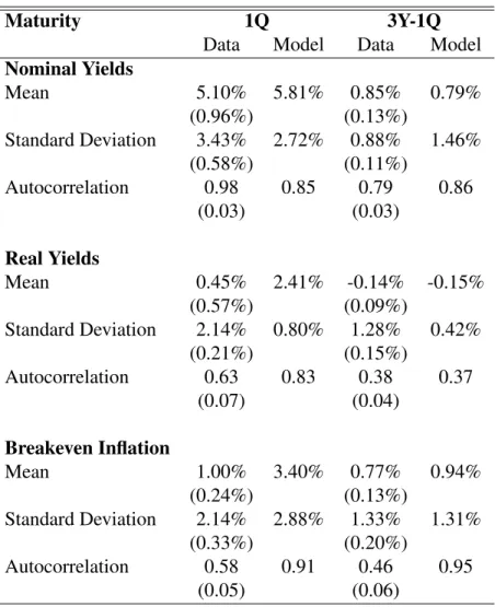
During the recession, stock prices fell -53%, as shown in Figure 7.2. From the start of the recession in 2007Q4 to the 2008Q3, the 3-month nominal and real bond yields fell -3.46% and -2.57%. At the ZLB over 2008Q4 to 2009Q1, the 3 year nominal bond yield fell, with short-term yields falling faster, causing a positive and increasing nominal spread. Real bond yields rose, with short-term yields rising faster, implying a negative real spread increasing in magnitude. Breakeven inflation, defined as the difference between nominal and real rates, fell and became negative. Short-term breakeven inflation yields fell faster, causing a positive and increasing inflation spread.
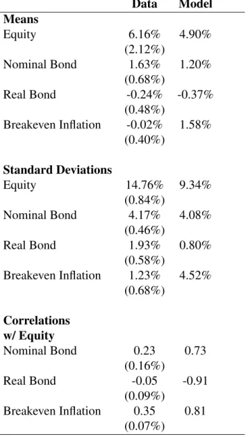
In addition to matching the dynamics observed during the Great Recession, the model also matches unconditional equity and bond market moments. Examining correlations between equity and bond markets, nominal and inflation excess returns are positively correlated with equity excess returns while real and equity excess returns are negatively correlated unconditionally. Using a long sample from the U.K., Bansal, Kiku, and Yaron (2012) show the real yield curve is downward sloping. Although real bonds have only been actively trading since 2004 in the U.S, the average quarterly yield spread between 3 year and 3 month real yields prior to the Great Recession is -0.14%. A downward sloping real curve implies that real bonds provide investors insurance by hedging declines in productivity and equity prices.
The empirical evidence during the Great Recession suggests the relationship between equity and real bonds are structurally different at the ZLB. Furthermore, it implies real bonds cease to provide investors portfolio insurance during extreme downturns, precisely when they value it most. The theoretical source of this time variation is investigated in the next sections.
While understanding the implications of constrained monetary policy is important, empirically it is difficult to measure due to the highly conditional nature of the ZLB and its infrequent ob-servations. In addition, real bonds in the U.S. have only been trading actively since 2004. Since measuring the potentially time-varying equity and bond market correlations at the ZLB is empiri-cally challenging, it is important to appeal to general equilibrium models to help interpret the data observed during the Great Recession and understand mechanisms at play.
CHAPTER 4: RESULTS
Calibration
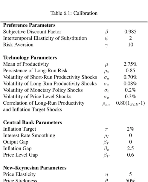
The model is calibrated to match 1) the unconditional quantity and asset pricing moments in the post-Bretton Woods era, 2) the empirical dynamics observed during the Great Recession, and 3) the conditional quantity and asset pricing moments at the ZLB. Over the 45 year span from 1971 to 2015, the Federal Reserve was at the effective ZLB (defined as less than 0.25% 3 month nominal yield) for 7 years from 2009 to 2015, or 15.6% of the sample. The benchmark calibration hits the effective ZLB 12.5% when simulated for a long sample.
The model is solved at a monthly frequency and annualized parameter values are reported. For the benchmark calibration, mean productivity growth is calibrated to match the unconditional consumption growth rate of 2.75%. Consistent with the long-run risk literature of Bansal and Yaron (2004) and Croce (2014), the intertemporal elasticity of substitution is 2, risk aversion is 10, and expected productivity growth shocks have an annual persistence of 0.85. The subjective discount factor is set to 0.985 and steady state labor hours is chosen to match the data in which 22%of total hours is devoted to working.
Consistent with the Taylor rule estimation in Table 6.12, the central bank places a weight of 2.5 on the inflation gap and 0.6 on the price level gap. The inflation target is set to 2% to match the Federal Reserve’s current long-run inflation target. As is standard in the New-Keynesian literature, price elasticity and stickiness parameters are chosen to imply an average 25% markup and 2 quarters of price stickiness.
consumption growth; while during the Great Recession, lower expected inflation is not correlated with higher expected consumption growth.
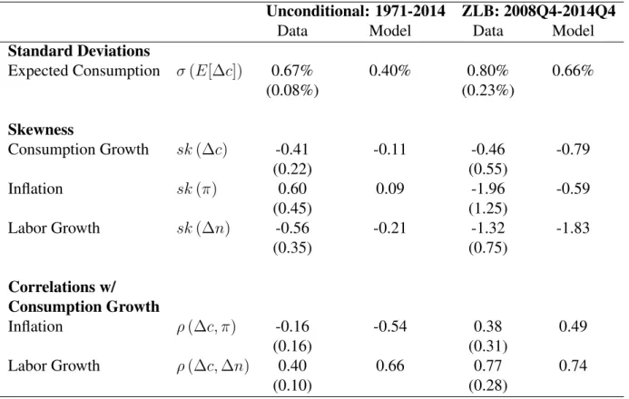
Unconditional Moments
The model matches the unconditional means of consumption growth and labor. As in the data, inflation volatility is relatively higher compared to consumption growth and the correlation between consumption and inflation is positive on average.
For unconditional yields, the model does well in matching the level of the 3 month nominal yield and the upward sloping nominal yield, as measured by the spread between the 3 year and 3 month nominal yield. As in the data, the standard deviation of the spread is less than the short rate. With respect to real yields, the model matches the small but negative real yield spread. Standard deviations and autocorrelations of the 3 year minus 3 month real spread are less than the 3 month real yield. Finally, the model matches the upward sloping breakeven inflation spread and standard deviations of the 3 month breakeven inflation yield and spread.
With respect to excess returns, the model matches the high equity risk premium, positive nom-inal bond risk premium, and negative real bond risk premium. In addition, the model matches nominal bond excess return volatility, and implies less volatile real bond excess returns relative to nominal bond excess returns. The model replicates the unconditional correlations of excess returns between equity and bond markets. During normal times, nominal bond and breakeven inflation ex-cess returns are positively correlated with equity exex-cess returns while real exex-cess are negatively correlated with equity excess returns.
The model is also consistent with the positive correlation between real yields and equity returns observed during the pre-Great Recession. Finally, the model matches both equity and real bond’s responses to long-run productivity shocks. Pre-crisis, both real rates and equity returns would fall in response to negative long-run productivity declines.
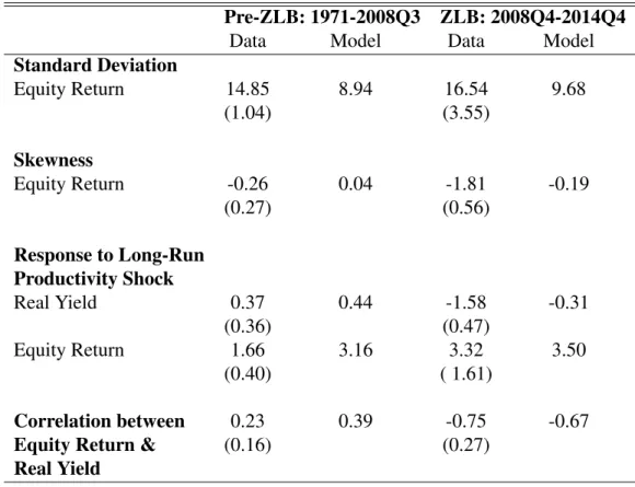
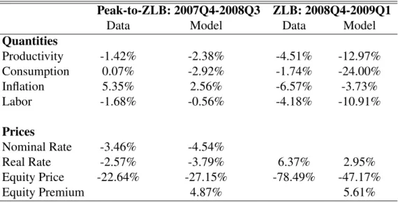
Great Recession Dynamics
to Table 6.7, the dynamics are broken up into two subperiods. In the first period, labeled ”Peak-to-ZLB”, the model replicates the dynamics that occurred in reaching the ZLB from 2007Q4 to 2008Q3. Cumulative productivity growth is negative and close to the -1.42% empirical counterpart, cumulative inflation is low but positive, and labor growth is negative. With respect to prices, equity price, 3 month nominal yield, and 3 month real yields fall by 23%, 4.5%, and 3.8% in the model compared to 23%, 3.5%, and 2.6% in the data.
In the second period when the nominal rate is constrained at the ZLB, productivity growth and labor growth decrease by 13% and 11% in the model compared to 4.5% and 4.2% in the data. As in the data, cumulative consumption growth is negative and both the data and model experience deflation. With respect to prices, equity prices fall by 47% while the 3 month real yield rises 3% in the model compared to 78% and 3% in the data, respectively. Finally, the model predicts that the equity risk premium increases 0.74% at the ZLB relative to the unconditional equity risk premium. Time-Varying ZLB Moments
The model is able to match conditional moments observed at the ZLB. With respect to quan-tities, inflation and labor growth become negatively skewed. Uncertainty of consumption growth, as measured by conditional volatility of expected consumption growth, increases. In addition, consumption and inflation become negatively correlated.
At the ZLB, the real bond’s rate response to long-run productivity shocks reverses. While real rates fall in normal times in response to a negative long-run productivity shock, real rates rise at the ZLB in response to a negative long-run productivity shock. Equity returns continue to fall at the ZLB. This time-varying response for real bonds produces a time varying correlation between real bonds and equity markets. Using filtered productivity shocks from the Great Recession, the model produces a negative correlation between real bonds and equities, consistent with the observed negative correlation in the data.
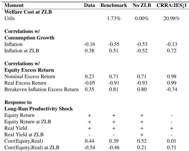
downside risk results in a time-varying, increasing equity risk premium at the ZLB. ZLB Predictions
Given that empirical observations of being at the ZLB are rare, it is important to appeal to structural models to help guide economists and policy makers’ assessment of the these extreme times. The model makes two important predictions. First, the equity risk premium is increasing at the ZLB. This channel has been explained above and is driven by the endogenous increase in uncertainty of macrofundamentals created by the ZLB. Second, policy makers face the question if the ZLB is an important constraint. The Federal Reserve seeks to stabilize short-run fluctuations in labor markets while maintaining a long-run moderate and stable inflation rate. Ex-ante it is unclear as to if the central bank should care about the costs of being constrained at the ZLB in the face of declining long-run productivity growth. Given the short-run focus of the central bank, a natural question to ask is how costly is the ZLB relative to normal times when we think about the subsequent 5 year recovery period following a shock at the ZLB. Specifically, define
ˆ
ut+j = ln ∂Ut+j
∂xt
Ut+j
L=
60
X
j=1 ˆ
uZLBt+j −uˆSSt+j
ˆ
Mechanisms
ZLB
In the model, intertemporal allocations depend on two channels: a wage channel and a savings channel. In response to a negative long-run supply news shock, wages fall and households supply less labor. To counteract this via the savings channel, the central bank lowers the nominal interest rate to stimulate aggregate demand and increase demand for labor. On net, the wage channel dom-inates and labor declines. Declining labor implies declining marginal costs and falling inflation.
At the ZLB, monetary policy becomes constrained and cannot further stimulate the economy, resulting in a liquidity trap. Households foresee falling future prices and delay current consump-tion, decreasing current aggregate demand and further decreasing demand for labor. Thus in nor-mal times, the savings channel counteracts the wage channel, while at the ZLB, the savings channel amplifies the effects of the wage channel. The liquidity trap at the ZLB results in larger declines in consumption, labor, and inflation with respect to negative long-run productivity news relative to normal times. Hence, the ZLB is characterized by negatively skewed and increasingly uncertain macrofundamentals.
Given the constraint of the ZLB, the real rate must rise to offset falling expected inflation. In equilibrium, future consumption growth increases due to the asymmetric response of labor’s re-sponse to the liquidity trap. In rere-sponse to a negative long-run supply shock at the ZLB, labor falls relatively more than in normal times. The negative skewness in the level of current labor im-plies positive future labor growth and hence positive future consumption growth. Increasing future consumption growth implies increasing future real rates via the nominal bond’s Euler equation. Finally, as equity is modeled as a levered consumption claim in the model, the negatively skewed consumption growth at the ZLB results in negatively skewed and more volatile equity returns. EZ Preferences
without Epstein Zin recursive preferences. Recursive preferences allow the IES to be disentangled from risk aversion. With CRRA preferences, risk aversion is equal the reciprocal of the IES. When the IES is less than 1, agents are relatively more impatient and the wealth effect dominates the sub-stitution effect, implying counterfactually investors use equity claims to provide insurance against bad times. In this case, the model’s equity risk premium is negative.
When the IES is greater than 1, the return to consumption falls in response to negative long-run supply news shocks, generating a positive equity risk premium. However, with CRRA preferences, risk aversion is less than 1 and the model’s implications are muted as investors do not sufficiently price the downside risk. As discussed in Bansal and Yaron (2004) and Colacito, Ghysels, Meng, and Siwasarit (2016), when the IES and risk aversion are allowed to both be greater than 1, in-vestors with EZ preferences dislike negatively skewed and increasing uncertain equity claims and command a higher risk premium relative to agents with CRRA preferences.
Holding risk aversion fixed at 10 and comparing the benchmark calibration to CRRA prefer-ences where IES is 101 , a negative 3 standard deviation long-run productivity shock at the ZLB re-sults in an increase in the equity risk premium by 0.40% and 0.01% for EZ and CRRA preferences, respectively. Hence having agents with EZ preferences is crucial to produce both qualitatively and quantitatively interesting asset pricing implications in response to the endogenous macroeconomic ZLB dynamics.
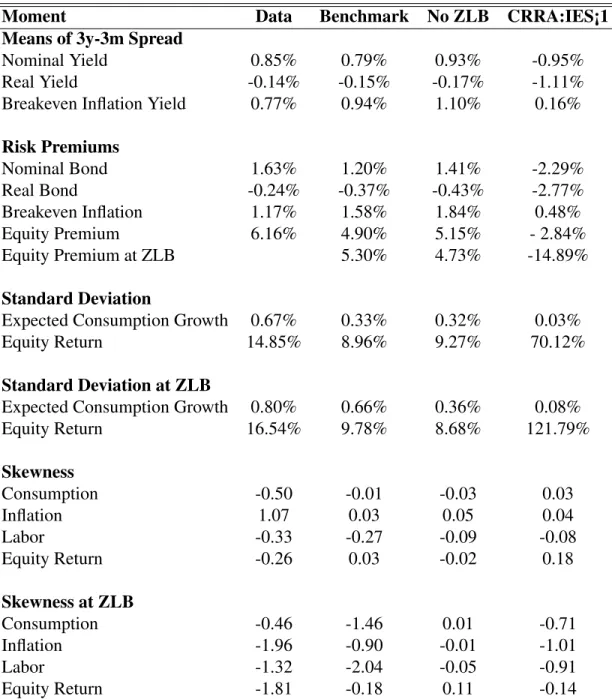
Sensitivity Analysis
No ZLB
CRRA: IES<1
With CRRA preferences, risk aversion is equal to the IES. Examining the impact of CRRA preferences when the IES is less than 1 and holding risk aversion to 10, we see the model fails to qualitatively reproduce many unconditional and conditional moments. Counterfactually, the nominal yield spread, nominal bond risk premium, and equity premium are negative. In addition, the calibration produces real bond excess returns that are strongly positively correlated with equity excess returns while breakeven inflation excess returns are negatively correlated with equity excess returns. Finally, equity returns rise in response to negative long-run productivity shocks, resulting in a positive correlation between real bond rates and equity returns at the ZLB.
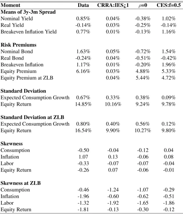
CRRA: IES>1
Examining the impact of CRRA preferences by holding the IES to 2, we see that the model produces quantitatively incorrect asset pricing moments. The nominal yield spread and equity pre-mium are low at 0.01% and 0.15%, while the nominal bond prepre-mium overshoots at 4.07%. The model predicts a very small increase in the equity risk premium at the ZLB. With EZ preferences, agents care about time-varying uncertainty and negatively skewed returns. With CRRA prefer-ences, this channel is absent and agents do not price the endogenous increasing macroeconomic uncertainty and negatively skewed consumption growth at the ZLB. Hence the increase in the eq-uity premium is magnitudes smaller than compared with EZ preferences. In regards to welfare, with CRRA preferences such that the IES=2, the short-run cost of constrained monetary policy is 7 magnitudes smaller than compared to EZ preferences.
Long-Run Productivity and Inflation Target Correlation
GHH Preferences&Interest Rate Smoothing
CHAPTER 5: CONCLUSION
I show that in a New-Keynesian model subject to the zero lower bound (ZLB), constrained monetary policy endogenously results in increasing risk premium and time-varying equity-bond market correlations. Liquidity traps at the ZLB are characterized by negatively skewed consump-tion growth, labor growth, and inflaconsump-tion. Negatively skewed consumpconsump-tion growth results in neg-atively skewed equity returns. Investors with recursive preferences price the increased downside risk, resulting in a greater equity risk premium. While real bond yields fall in response to produc-tivity declines in normal times, real bond yields increase at the ZLB in response to falling expected inflation. Hence, equity returns and real bond yields become negatively correlated at the ZLB, while positive in normal times.
TABLES
Table 6.1: Calibration Preference Parameters
Subjective Discount Factor β 0.985
Intertemporal Elasticity of Substitution ψ 2
Risk Aversion γ 10
Technology Parameters
Mean of Productivity µ 2.75%
Persistence of Long-Run Risk ρa 0.85 Volatility of Short-Run Productivity Shocks σa 0.70% Volatility of Long-Run Productivity Shocks σx 0.08% Volatility of Monetary Policy Shocks σi 0.2% Volatility of Price Level Shocks σπ 0.3% Correlation of Long-Run Productivity ρx,π 0.80(1ZLB-1) and Inflation Target Shocks
Central Bank Parameters
Inflation Target π 2%
Interest Rate Smoothing ρI 0
Output Gap βY 0
Inflation Gap βπ 2.5
Price Level Gap βP 0.6
New-Keynesian Parameters
Price Elasticity η 5
Price Stickiness θ 50%
Table 6.2: Macroeconomic Quantity Statistics Data Model Means
Consumption Growth E[∆c] 2.75% 2.75% (0.29%)
Inflation E[π] 4.08% 2.00%
(0.79%)
Labor E[N] 0.22% 0.22%
(0.003%)
Standard Deviations
Consumption Growth σ(∆c) 0.90% 1.27% (0.08%)
Inflation σ(π) 1.71% 1.47%
(0.27%)
Labor Growth σ(∆N) 1.41% 0.86% (0.12%)
Autocorrelations
Consumption Growth ρ(∆c) 0.52 0.19 (0.10)
Inflation ρ(π) 0.62 0.95
(0.15)
Labor ρ(N) 0.99 0.63
(0.10)
Table 6.3: Time-Varying Macroeconomic Quantity Statistics
Unconditional: 1971-2014 ZLB: 2008Q4-2014Q4
Data Model Data Model
Standard Deviations
Expected Consumption σ(E[∆c]) 0.67% 0.40% 0.80% 0.66%
(0.08%) (0.23%)
Skewness
Consumption Growth sk(∆c) -0.41 -0.11 -0.46 -0.79
(0.22) (0.55)
Inflation sk(π) 0.60 0.09 -1.96 -0.59
(0.45) (1.25)
Labor Growth sk(∆n) -0.56 -0.21 -1.32 -1.83
(0.35) (0.75)
Correlations w/ Consumption Growth
Inflation ρ(∆c, π) -0.16 -0.54 0.38 0.49
(0.16) (0.31)
Labor Growth ρ(∆c,∆n) 0.40 0.66 0.77 0.74
(0.10) (0.28)
Table 6.4: Yield Statistics
Maturity 1Q 3Y-1Q
Data Model Data Model Nominal Yields
Mean 5.10% 5.81% 0.85% 0.79%
(0.96%) (0.13%)
Standard Deviation 3.43% 2.72% 0.88% 1.46% (0.58%) (0.11%)
Autocorrelation 0.98 0.85 0.79 0.86
(0.03) (0.03)
Real Yields
Mean 0.45% 2.41% -0.14% -0.15%
(0.57%) (0.09%)
Standard Deviation 2.14% 0.80% 1.28% 0.42% (0.21%) (0.15%)
Autocorrelation 0.63 0.83 0.38 0.37
(0.07) (0.04)
Breakeven Inflation
Mean 1.00% 3.40% 0.77% 0.94%
(0.24%) (0.13%)
Standard Deviation 2.14% 2.88% 1.33% 1.31% (0.33%) (0.20%)
Autocorrelation 0.58 0.91 0.46 0.95
(0.05) (0.06)
Table 6.5: Excess Return Statistics Data Model Means
Equity 6.16% 4.90%
(2.12%)
Nominal Bond 1.63% 1.20% (0.68%)
Real Bond -0.24% -0.37%
(0.48%)
Breakeven Inflation -0.02% 1.58% (0.40%)
Standard Deviations
Equity 14.76% 9.34%
(0.84%)
Nominal Bond 4.17% 4.08% (0.46%)
Real Bond 1.93% 0.80%
(0.58%)
Breakeven Inflation 1.23% 4.52% (0.68%)
Correlations w/ Equity
Nominal Bond 0.23 0.73
(0.16%)
Real Bond -0.05 -0.91
(0.09%)
Breakeven Inflation 0.35 0.81 (0.07%)
Table 6.6: Time-Varying Return Statistics
Pre-ZLB: 1971-2008Q3 ZLB: 2008Q4-2014Q4
Data Model Data Model
Standard Deviation
Equity Return 14.85 8.94 16.54 9.68
(1.04) (3.55)
Skewness
Equity Return -0.26 0.04 -1.81 -0.19
(0.27) (0.56)
Response to Long-Run Productivity Shock
Real Yield 0.37 0.44 -1.58 -0.31
(0.36) (0.47)
Equity Return 1.66 3.16 3.32 3.50
(0.40) ( 1.61)
Correlation between 0.23 0.39 -0.75 -0.67 Equity Return & (0.16) (0.27)
Real Yield
Table 6.7: ZLB Dynamics
Peak-to-ZLB: 2007Q4-2008Q3 ZLB: 2008Q4-2009Q1
Data Model Data Model
Quantities
Productivity -1.42% -2.38% -4.51% -12.97%
Consumption 0.07% -2.92% -1.74% -24.00%
Inflation 5.35% 2.56% -6.57% -3.73%
Labor -1.68% -0.56% -4.18% -10.91%
Prices
Nominal Rate -3.46% -4.54%
Real Rate -2.57% -3.79% 6.37% 2.95%
Equity Price -22.64% -27.15% -78.49% -47.17%
Equity Premium 4.87% 5.61%
Table 6.8: Sensitivity Analysis: Part 1
Moment Data Benchmark No ZLB CRRA:IES¡1 Means of 3y-3m Spread
Nominal Yield 0.85% 0.79% 0.93% -0.95%
Real Yield -0.14% -0.15% -0.17% -1.11%
Breakeven Inflation Yield 0.77% 0.94% 1.10% 0.16%
Risk Premiums
Nominal Bond 1.63% 1.20% 1.41% -2.29%
Real Bond -0.24% -0.37% -0.43% -2.77%
Breakeven Inflation 1.17% 1.58% 1.84% 0.48%
Equity Premium 6.16% 4.90% 5.15% - 2.84%
Equity Premium at ZLB 5.30% 4.73% -14.89%
Standard Deviation
Expected Consumption Growth 0.67% 0.33% 0.32% 0.03%
Equity Return 14.85% 8.96% 9.27% 70.12%
Standard Deviation at ZLB
Expected Consumption Growth 0.80% 0.66% 0.36% 0.08%
Equity Return 16.54% 9.78% 8.68% 121.79%
Skewness
Consumption -0.50 -0.01 -0.03 0.03
Inflation 1.07 0.03 0.05 0.04
Labor -0.33 -0.27 -0.09 -0.08
Equity Return -0.26 0.03 -0.02 0.18
Skewness at ZLB
Consumption -0.46 -1.46 0.01 -0.71
Inflation -1.96 -0.90 -0.01 -1.01
Labor -1.32 -2.04 -0.05 -0.91
Equity Return -1.81 -0.18 0.11 -0.14
Table 6.9: Sensitivity Analysis: Part 2
Moment Data CRRA:IES¿1 ρ=0 CES:f=0.5
Means of 3y-3m Spread
Nominal Yield 0.85% 0.04% -0.38% 1.02%
Real Yield -0.14% 0.03% -0.25% -0.14%
Breakeven Inflation Yield 0.77% 0.01% -0.13% 1.16%
Risk Premiums
Nominal Bond 1.63% 0.05% -0.72% 1.54%
Real Bond -0.24% 0.04% -0.51% -0.42%
Breakeven Inflation 1.17% 0.01% -0.20% 1.96%
Equity Premium 6.16% 0.03% 4.88% 5.33%
Equity Premium at ZLB 0.04% 5.44% 4.72%
Standard Deviation
Expected Consumption Growth 0.67% 0.33% 0.38% 0.09%
Equity Return 14.85% 10.16% 9.24% 9.78%
Standard Deviation at ZLB
Expected Consumption Growth 0.80% 0.40% 0.56% 0.12%
Equity Return 16.54% 9.90% 10.27% 9.80%
Skewness
Consumption -0.50 -0.04 -0.12 0.04
Inflation 1.07 0.13 -0.06 0.08
Labor -0.33 -0.07 -0.07 -0.04
Equity Return -0.26 0.07 -0.06 -0.01
Skewness at ZLB
Consumption -0.46 -1.24 -1.07 -0.29
Inflation -1.96 -0.60 -0.62 -0.51
Labor -1.32 -1.92 -1.65 -1.86
Equity Return -1.81 -0.13 -0.30 -0.12
Table 6.10: Sensitivity Analysis: Part 3
Moment Data Benchmark No ZLB CRRA:IES¡1 Welfare Cost at ZLB
Utils 1.73% 0.00% 20.98%
Correlations w/ Consumption Growth
Inflation -0.16 -0.55 -0.53 -0.13
Inflation at ZLB 0.38 0.51 -0.52 0.72
Correlations w/ Equity Excess Return
Nominal Excess Return 0.23 0.71 0.71 0.98
Real Excess Return -0.05 -0.91 -0.93 0.99
Breakeven Inflation Excess Return 0.35 0.81 0.80 -0.74
Response to
Long-Run Productivity Shock
Equity Return + + +
-Equity Return at ZLB + + +
-Real Yield + + + +
Real Yield at ZLB - - +
-Corr(Equity,Real) 0.44 0.39 0.52 0.01
Corr(Equity,Real) at ZLB -0.54 -0.46 0.21 0.71
Table 6.11: Sensitivity Analysis: Part 4
Moment Data CRRA:IES¿1 ρ=0 CES:f=0.5
Welfare Cost at ZLB
Utils 0.25% 1.03% 0.38%
Correlations w/ Consumption Growth
Inflation -0.16 -0.54 0.05 -0.44
Inflation at ZLB 0.38 0.09 0.37 -0.04
Correlations w/ Equity Excess Return
Nominal Excess Return 0.23 0.71 -0.03 0.77
Real Excess Return -0.05 -0.92 -0.86 -0.79
Breakeven Inflation Excess Return 0.35 0.80 0.17 0.85
Response to
Long-Run Productivity Shock
Equity Return + + + +
Equity Return at ZLB + + + +
Real Yield + + + +
Real Yield at ZLB - - -
-Corr(Equity,Real) 0.44 0.52 0.07 0.45
Corr(Equity,Real) at ZLB -0.54 -0.49 -0.43 -0.22
Table 6.12: Taylor Rule Estimation Policy Parameter
Interest Rate Smoothing ρi 0.88 (0.03)
Output Gap βY -0.02 0.15
(0.13) (0.05) Inflation Gap βπ 2.47 0.63
(0.26) (0.13) Price Level Gap βP 0.62 -0.01
(0.19) (0.08)
FIGURES
Figure 7.1: Quantities
2007 2008 2009 2010 -5
0 5
Productivity Growth
∆ a E[∆a]
2007 2008 2009 2010 -2
0 2
Consumption Growth
∆ c E[∆c]
2007 2008 2009 2010 1
2 3 4 5
Federal Funds Rate
2007 2008 2009 2010 -5
0 5
Inflation
2007 2008 2009 2010 0.205
0.21 0.215 0.22
Hours Worked
2007 2008 2009 2010 0.4
0.6 0.8
Consumption Growth Uncertainty
Figure 7.2: Returns
2007 2008 2009 2010
0
5 Nominal Yield
2007 2008 2009 2010
0 2 4 6 8
Real Yield
2007 2008 2009 2010
-8 -6 -4 -2 0 2
Breakeven Inflation
2007 2008 2009 2010
-20 0 20
Equity Return
Figure 7.3: IRF: Quantities
-0.5
0 Expected Productivity Growth
Normal ZLB
-0.5
0 Productivity Growth
-0.4 -0.2
0 Hours Worked
-6 -4 -2 0
Consumption Growth
0 2 4 6 8 10 12
Months -0.8
-0.6 -0.4 -0.2 0
Inflation
Figure 7.4: IRF: Fisher Decomposition
-0.8 -0.6 -0.4 -0.2
Expected Productivity Growth
Normal ZLB
-0.4 -0.2
0 Nominal Interest Rate
-0.4 -0.2
0 Hours Worked
-0.4 -0.2 0
Expected Inflation
0 5 10
Months -0.5
0 0.5
Expected Consumption Growth
0 5 10
Months -0.2
0 0.2 0.4
Real Interest Rate
Figure 7.5: IRF: Returns
-0.8 -0.6 -0.4 -0.2
Expected Productivity Growth
Normal ZLB
-0.4 -0.2
0 Nominal Interest Rate
0 2 4
Real Stochastic Discount Factor
-0.2 0 0.2 0.4
Real Interest Rate
0 5 10
Months -30
-20 -10
0 Equity Return
0 5 10
Months -0.4
-0.2 0
Breakeven Inflation
Figure 7.6: IRF: Stochastic Discount Factor
-0.5
0 Expected Productivity Growth
Normal ZLB
-0.5 0 0.5
Expected Consumption Growth
0 2 4
Real Stochastic Discount Factor
0 2 4
EZ
0 2 4 6 8 10 12
Months 0
0.2 0.4 0.6
CRRA
Figure 7.7: IRF: Consumption Growth Moments
-6 -4 -2 0
Consumption Growth ∆c
t
Normal ZLB
0 0.5 1 1.5
Volatility of Consumption Growth Vol
t[∆ct+1]
-0.5 0 0.5
Expected Consumption Growth E
t[∆ct+1]
0 2 4 6 8 10 12
Months 0
0.5 1
×10Volatility of Expected Consumption Growth Vol-3 t(Et+1[∆ct+2])
Figure 7.8: IRF: Equity Risk Premium
-20 -10 0
∆ Excess Equity Returns
0 0.5 1 1.5
Volatility of Expected Equity Returns
Normal ZLB
0 2 4 6 8 10 12
Months 0
0.1 0.2
Equity Risk Premium
APPENDIX A: ROBUSTNESS STATISTICS
Table A.1: Yield Statistics Implied by Inflation Swaps
Maturity 1Q 3Y-1Q
Real Yields
Mean -0.18% 0.18%
(0.51%) (0.04%) Standard Deviation 3.26% 1.47%
(0.16%) (0.07%) Autocorrelation 0.77 0.43
(0.07%) (0.07%)
Breakeven Inflation
Mean 1.63% 0.44%
(0.20%) (0.08%) Standard Deviation 2.82% 0.73%
(0.23%) (0.11%) Autocorrelation 0.67 0.58
(0.06%) (0.08%)
Table A.2: Excess Return Statistics Implied by Inflation Swaps Data
Means
Real Bond -0.22%
(0.39%) Breakeven Inflation -0.04%
(0.31%)
Standard Deviations
Real Bond 2.61%
(0.50%) Breakeven Inflation 2.41%
(0.55%)
Correlations w/ Equity Market
Real Bond -0.36
(0.09%) Breakeven Inflation 0.53
(0.07%)
Table A.3: Time-Varying Return Statistics Implied by Inflation Swaps Pre-ZLB: 2004-2008Q3 ZLB: 2008Q4-2014Q4 Response to Long-Run
Productivity Shock
Real Yield 0.36 -0.85
(0.34) (0.30)
Correlation between 0.41 -0.61
Equity Return & (0.11) (0.20) Real Yield
APPENDIX B: EULER ERRORS
Figure B.1: Nominal Bond Euler Errors
-3 -2 -1 0 1 2 3
Expected Productivity Growth Standard Deviation
0 0.2 0.4 0.6 0.8 1 1.2
Percent Error Relative to Nominal Interest Rate Steady State
Average Error Maximum Error ZLB
APPENDIX C: MODEL DERIVATION
Households
Households choose consumption Ct, leisureLt, nominal bond holdingsBt, and labor supply Ntto maximize lifetime utilityU0, where
Ut=
"
(1−β) ˜C1−
1
ψ
t +βEt
Ut1+1−γ
1−1
ψ
1−γ
# 1
1−1
ψ
˜ Ct=
ϕC1−
1
f
t + (1−ϕ) (AtLt)1
−1
f
1
1−1
f
CES
Ctϕ(AtLt)1
−ϕ
CDf = 1 Ct−ϕAt
Nt1+ 1f
1+f1 GHH 1≥Nt+Lt
whereAtdenotes labor-augmenting productivity. The household’s budget constraint is
PtCt+QtBt+1 ≤Bt+WtNt
The household takes the price of consumptionPt, the price of nominal bondsQt, and the nominal wage rateWtas given. Nominal bonds are discount bonds and payoff $Btdollars at time t. The price of the nominal bond is the invesrse of the nominal interest rate,Qt= If
−1
t . The Lagrangian is
L =U0 +· · ·
+λ1,t[Bt+WtNt−PtCt−QtBt+1] +λ2,t[1−Nt−Lt]
The FOC w.r.t. consumption is
∂L ∂Ct
=∂U0 ∂Ct
−λ1,tPt = 0 λ1,tPt=
∂U0 ∂Ct
The real SDF is
Mt+1 =
∂U0/∂Ct+1 ∂U0/∂Ct
=
β∆ ˜C
1
f−
1
ψ t+1 ∆C
−1
f t+1
Ut+1
Et[Ut1+1−γ] 1 1−γ
!ψ1−γ
CES
β∆C−
1
ψ t+1
Ut+1
Et[Ut1+1−γ] 1 1−γ
!ψ1−γ
CDf = 1
β∆ ˜C−
1
ψ t+1
Ut+1
Et[Ut1+1−γ] 1 1−γ
!ψ1−γ
GHH
The FOC w.r.t. leisure is
∂L ∂Lt
=∂U0 ∂Lt
−λ2,t = 0 λ2,t =
∂U0 ∂Lt
The FOC w.r.t. labor is
∂L ∂Nt
=λ1,tWt−λ2,t = 0 Wt =
The FOC w.r.t. nominal bonds is
∂L ∂Bt+1
=Et[λ1,t+1]−Qtλ1,t = 0 Qt=Et
λ1,t+1 λ1,t
=Et
Mt+1 Πt+1
whereΠt+1 = PPt+1t is the inflation rate. The real and nominal Euler bond equations are
Rft =Et[Mt+1]
−1
Itf =Et
Mt+1 Πt+1
−1
whereRft is the real risk-free interest rate. Final Goods Firm
A final goods firm buys intermediate goodsYit to produce final goodsYtto maximize profits. It takes intermediate goods pricesPit and final goods pricePt as given. It producesYtwith CES technology
Yt=
Z 1
0 Y1−
1
η it di
1−11
η
Specifically, the final goods firm maximizes
max Yit
PtYt−
Z 1
0
PitYitdi
s.t. Yt =
Z 1
0 Y1−
1
η it di
1−11
The Lagrangian is
L =Pt
Z 1
0 Y1−
1
η it di
1
1−1η
−
Z 1
0
PitYitdi
The FOC w.r.t. intermediate goods
∂L ∂Yit
=Pt
Yt Yit
1η
−Pit= 0
Yit =
Pit Pt
−η
Yt
The price index is
PtYt=
Z 1
0
PitYitdi
= Z 1 0 Pit Pit Pt −η
Ytdi
Pt=
Z 1
0
Pit1−ηdi
1−1η
Intermediate Goods Firms
Monopolistically competitive firms choose labor Nit and price Pit and produce intermediate goodsYit to maximize discounted real profits. Firms take wages as given and use constant return to scales production technologies
Specifically firms maximize
max
{Nit,Pit}
Et
" ∞ X
j=0 Mt,t+j
Pi,t+jYi,t+1−Wt+jNi,t+j Pt+j
#
s.t. Yit =AtNit Yit ≥
Pit Pt
−η
Yt
The Lagrangian is
L =Et
" ∞ X
j=0 Mt,t+j
Pi,t+jYi,t+j −WtNi,t+j Pt+j
#
+· · ·
+λ1,t(Fit−Yit) +λ2,t Yit−
Pit Pt −η Yt ! +· · ·
The FOC w.r.t. to labor is
∂L ∂Nit
=− Wt Pt
+λ1,tFN,it = 0 Wt
Pt
=λ1,tFN,it
Note that Ptλ1,t = M Ctare the firms’ nominal marginal costs. Firms’ prices are assumed to be stickya`la Calvo. Each period, firms can update their pricePitwith probability1−θ. Firms choose the best pricePitat timetknowing that they will not be able to reoptimize in the next period with probabilityθ, i.e. they maximize
max Pit Et " ∞ X j=0
θjMt,t+j Pt+j
(PitYi,t+j−Wt+jNi,t+j)
Substituting in demand for labor and output, note that
PitYi,t+j −Wt+jNi,t+j =PitYi,t+j−M Ct+jYi,t+j = (Pit−M Ct+j)
Pit Pt+j
−η
Yt+j
= Pit1−η −M Ct+jPit−η
Ptη+jYt+j
The Lagrangian is
L =Et
" ∞ X
j=0
θjMt,t+j P 1−η
it −M Ct+jP
−η it
Ptη+−j1Yt+j
#
The FOC w.r.t. firm’s price is
∂L ∂Pit
=Et
" ∞ X
j=0
θjMt,t+j (1−η)Pit−η +ηM CtPit−η−1
Ptη+−j1Yt+j
# = 0 This implies Pit Pt = η η−1
Et
h P∞
j=0θjMt,t+j
P
t+j Pt
η
Yt+jmct+j
i
Et
P∞
j=0θjMt,t+j
Pt+j Pt
η−1
Yt+j
where mct = M CPtt are real marginal costs. The firm’s price setting equation can be written re-currsively as
Pt∗ = η η−1
ζt ξt
ζt=mct·Yt+θEt
Mt+1Πηt+1ζt+1
ξt=Yt+θEt
Mt+1Πηt+1−1ξt+1
Government
Monetary policy follows a Taylor (1993) rule
Itf I =
Itf−1 I
!ρI" Yt ¯ Yt βY Πt Π βπ Pt ¯ Pt
βP#1−ρI
eεi,t
Yt ¯ Yt
=∆Yt ∆Y
Yt−1 ¯ Yt−1 Pt
¯ Pt
=Π¯t Πt
Pt−1 ¯ Pt−1 ¯
Πt =Πexπ,t xπ,t =ρπxπ,t+επ,t
whereεi,tandεπ,tare monetary policy and inflation target shocks. Equilibrium
The aggregate resource constraint
Yt=Ct Yt=
Ft St
where price dispersion is
St = (1−θ)P
∗−η t +θΠ
η tSt−1
Prices follow
Technology
Technology evolves according to
REFERENCES
Adam, K. and R. M. Billi (2006). Optimal Monetary Policy Under Commitment with a Zero Bound on Nominal Interest Rates. Journal of Money, Credit, and Banking 38(7), 1877–1905. Bansal, R., D. Kiku, and A. Yaron (2012). An empirical evaluation of the long-run risks model for
asset prices. Critical Finance Review 1(2), 183–221.
Bansal, R. and I. Shaliastovich (2013, nov). A Long-Run Risks Explanation of Predictability Puzzles in Bond and Currency Markets. Review of Financial Studies 26(1), 1–33.
Bansal, R. and A. Yaron (2004). Risks for the Long Run: A Potential Resolution of Asset Pricing Puzzles. Journal of Finance 59(4), 1481–1509.
Basu, S. and B. Bundick (2015). Endogenous Volatility at the Zero Lower Bound : Implications for Stabilization Policy. Working Paper.
Bekaert, G., S. Cho, and A. Moreno (2010, nov). New Keynesian Macroeconomics and the Term Structure. Journal of Money, Credit and Banking 42(1), 33–62.
Black, F. (1995, nov). Interest Rates as Options. The Journal of Finance 50(5), 1371–1376. Calvo, G. A. (1983). Staggered prices in a utility-maximizing framework. Journal of monetary
Economics 12(3), 383–398.
Campbell, J., C. Pflueger, and L. M. Viceira (2015). Monetary policy drivers of bond and equity risks. Working Paper.
Campbell, J., R. Shiller, and L. Viceira (2009). Understanding inflation-indexed bond markets. Technical report.
Campbell, J., A. Sunderam, and L. M. Viceira (2013). Inflation bets or deflation hedges? The changing risks of nominal bonds. Technical report.
Clarida, R., J. Gal´ı, and M. Gertler (1999). The Science of Monetary Policy: A New Keynesian Perspective. Journal of Economic Literature 37(4), 1661–1707.
Colacito, R., E. Ghysels, J. Meng, and W. Siwasarit (2016). Skewness in Expected Macro Funda-mentals and the Predictability of Equity Returns: Evidence and Theory.The Review of Financial Studies.
Coleman, J. (1990, nov). Solving the Stochastic Growth Model by Policy-Function Iteration. Journal of Business & Economic Statistics 8(1), 27–29.
Epstein, L. G. and S. E. Zin (1989). Substitution, risk aversion, and the temporal behavior of consumption and asset returns: A theoretical framework. Econometrica: Journal of the Econo-metric Society, 937–969.
Fernald, J. (2014). Productivity and Potential Output Before, During, and After the Great Reces-sion. Technical report.
Fern´andez-Villaverde, J., G. Gordon, P. Guerr´on-Quintana, and J. Rubio-Ram´ırez (2015, nov). Nonlinear adventures at the zero lower bound. Journal of Economic Dynamics and Con-trol 57(12), 182–204.
Kim, D. H. and K. Singleton (2012, nov). Term structure models and the zero bound: an empirical investigation of Japanese yields. Journal of Econometrics 170(1), 32–49.
Krugman, P. (1998). It’s baaack: Japan’s slump and the return of the liquidity trap. Brookings Papers on Economic Activity 1998(2), 137–205.
Kung, H. (2015, nov). Macroeconomic linkages between monetary policy and the term structure of interest rates. Journal of Financial Economics 115(1), 42–57.
Li, E. X. and F. Palomino (2014). Nominal rigidities, asset returns, and monetary policy. Journal of Monetary Economics 66, 210–225.
Nakata, T. (2012). Uncertainty at the Zero Lower Bound. pp. 1–37.
Ohanian, L. E. and A. Raffo (2012). Aggregate hours worked in OECD countries: New measure-ment and implications for business cycles. Journal of Monetary Economics 59(1), 40–56. Pflueger, C. and L. M. Viceira (2016). Return Predictability in the Treasury Market: Real rates,
Inflation, and Liquidity. InHandbook of Fixed-Income Securities, Chapter 10. Wiley.
Piazzesi, M. and M. Schneider (2007). Equilibrium yield curves. In NBER Macroeconomics Annual 2006, Volume 21, Volume 21, pp. 389–472. MIT Press.
Rudebusch, G. D. and T. Wu (2008). A macro-finance model of the term structure, monetary policy and the economy. Economic Journal 118(530), 906–926.
Schmitt-Groh´e, S. and M. Uribe (2007, nov). Optimal simple and implementable monetary and fiscal rules. Journal of Monetary Economics 54(6), 1702–1725.
Swanson, E. and G. D. Rudebusch (2012). The Bond Premium in a DSGE Model with Long-Run Real and Nominal Risks. American Economic Journal: Macroeconomics 4(1), 1–5.
Swanson, E. and J. C. Williams (2014). Measuring the effect of the zero lower bound on medium-and longer-term interest rates. American Economic Review 104(10), 3154–3185.
![Table 6.2: Macroeconomic Quantity Statistics Data Model Means Consumption Growth E [∆c] 2.75% 2.75% (0.29%) Inflation E [π] 4.08% 2.00% (0.79%) Labor E [N ] 0.22% 0.22% (0.003%) Standard Deviations Consumption Growth σ (∆c) 0.90% 1.27% (0.08%) Inflation σ](https://thumb-us.123doks.com/thumbv2/123dok_us/8246180.2185188/34.918.262.658.306.834/macroeconomic-statistics-consumption-inflation-standard-deviations-consumption-inflation.webp)