MPI Implementation Analysis - A Practical Approach to Network Marketing

(1)

Optimizing MPI Collective Communication by

Orthogonal Structures

Matthias K¨

uhnemann

Fakultät für Informatik Technische Universität Chemnitz

09107 Chemnitz, Germany [email protected]–chemnitz.de

Thomas Rauber

Fakultät für Mathematik und Physik Universität Bayreuth

95445 Bayreuth, Germany rauber@uni–bayreuth.de

Gudula R¨

unger

Fakultät für Informatik Technische Universität Chemnitz

09107 Chemnitz, Germany [email protected]–chemnitz.de

Abstract

Many parallel applications from scientific computing use MPI collective com-munication operations to collect or distribute data. Since the execution times of these communication operations increase with the number of participating proces-sors, scalability problems might occur. In this article, we show for different MPI implementations how the execution time of collective communication operations can be significantly improved by a restructuring based on orthogonal processor struc-tures with two or more levels. As platform, we consider a dual Xeon cluster, a Beowulf cluster and a Cray T3E with different MPI implementations. We show that the execution time of operations like MPI Bcast or MPI Allgather can be re-duced by 40% and 70% on the dual Xeon cluster and the Beowulf cluster. But also on a Cray T3E a significant improvement can be obtained by a careful selection of the processor groups. We demonstrate that the optimized communication oper-ations can be used to reduce the execution time of data parallel implementoper-ations of complex application programs without any other change of the computation and communication structure. Furthermore, we investigate how the execution time of orthogonal realization can be modeled using runtime functions. In particular, we consider the modeling of two-phase realizations of communication operations. We present runtime functions for the modeling and verify that these runtime functions can predict the execution time both for communication operations in isolation and in the context of application programs.

(2)

1 Introduction

Parallel machines with distributed address space are widely used for the implementation of applications from scientific computing, since they provide good performance for a rea-sonable price. Portable message-passing programs can be written using message-passing standards like MPI or PVM. For many applications, like grid-based computations, a data-parallel execution usually leads to good performance. But for target machines with a large number of processors, data parallel implementations may lead to scalability problems, in particular when collective communication operations are frequently used for exchanging data. Often scalability can be improved by re-formulating the program as a mixed task and data parallel implementation. This can be done by partitioning the computations into multiprocessor tasks and by assigning the tasks to disjoint processor groups for execution such that one task is executed by the processors of one group in a data parallel way, but different independent tasks are executed concurrently by disjoint processor groups [16]. The advantage of a group-based execution is caused by the communication overhead of collective communication operations whose execution time shows a logarithmic or linear dependence on the number of participating processors, depending on the communication operation and the target machine.

Another approach to reduce the communication overhead is the use of orthogonal proces-sor groups [14] which are based on an arrangement of the set of procesproces-sors as a virtual two-or higher-dimensional grid and a fixed number of decompositions into disjoint processtwo-or subsets representing hyper-planes. To use orthogonal processor groups the application has to be re-formulated such that it consists of tasks that are arranged in a two- or higher-dimensional task grid that is mapped onto the processor grid. The execution of the program is organized in phases. Each phase is executed on a different partitioning of the processor set and performs communication in the corresponding processor groups only. For many applications, this may reduce the communication overhead considerably but requires a specific potential of parallelism within the application and a complete rearrangement of the resulting parallel program.

In this article we consider a different approach to reduce the communication overhead. Instead of rearranging the entire program to a different communication structure, we use the communication structure given in the data parallel program. But for each collective communication operation, we introduce an internal structure that uses an orthogonal ar-rangement of the processor set with two or more levels. The collective communication is split into several phases each of which exploits a different level of the processor groups. Using this approach a significant reduction in the execution time can be observed for different target platforms and different MPI implementations. The most significant im-provement results for MPI Allgather() operations. This is especially important as these operations are often used in scientific computing. Examples are iterative methods where MPI Allgather()operations are used to collect data from different processors and to make this data available to each processor for the next time step. The advantage of the approach is that the application does not have to provide a specific potential of parallelism and that all programs using collective communication can take advantage of the improved commu-nication. Also no rearrangement of the program is necessary and no specific knowledge about the additional implementation structure is needed, so that a data parallel imple-mentation mainly remains unchanged.

The internal rearrangement of the collective communication operations is done on top of MPI on the application programmers level. So, the optimization can be used on a large range of machines providing MPI. As target platforms we consider a Cray T3E, a Xeon cluster and a Beowulf cluster. As application programs we consider an iterative solution method for linear equation systems and solution methods for initial value problems of

(4)

ordinary differential equations.

Furthermore, we consider the modeling of the parallel runtime with runtime functions that are structured according to the orthogonal communication phases. This model is suitable for data parallel programs [15] as well as for mixed task and data parallel programs [11], and it can also be used for large and complicated application programs [8]. We investigate the use of runtime functions for modeling the runtime of MPI collective communication operations with the specific internal realization that is based on an orthogonal structuring of the processors in a two-dimensional grid. Using the runtime functions, the programmer can get an a priori estimation of the execution time to predict various runtime effects of an orthogonal realization.

The rest of the paper is organized as follows. Section 2 describes how collective com-munication operations can be arranged such that they consist of different steps, each performed on a subset of the entire set of processors. Section 3 presents the improvement in execution time obtained by such an arrangement on three different target platforms. Section 4 presents runtime functions to predict the behavior of execution time for collec-tive communication operation based on orthogonal group structure. Section 5 applies the improved operations in the context of larger application programs and shows the resulting improvements. Section 6 discusses related work and Section 7 concludes the paper.

2 Orthogonal structures for realizing communication

operations

The Message Passing Interface (MPI) standard has been defined in an effort to standardize the programming interface presented to developers arcoss a wide variety of parallel ar-chitectures. Many implementations of the standard are available, including highly-tuned versions for proprietary massively-parallel processors (MPPs), such as the Cray T3E, as well as hardware-independent implementations such as MPICH [4] and LAM-MPI [13], which have been ported to run on a large variety of machine types.

Most MPI implementations have been ported to cluster platforms, since clusters of com-modity systems connected by a high-speed network in a rather loosely-coupled MPP are a cost effective alternative to supercomputers. As the implementations are not tuned towards a specific architecture interconnection network, such realizations of MPI com-munication operations can be inefficient for some comcom-munication operations on some platforms. Especially the network topology is crucial for an efficient realization of a given communication pattern. Furthermore, the latency and bandwidth of the interconnection network determine the switch between different communication protocols, e.g. for short and long messages.

In this section we describe how collective communication operations can be realized in consecutive phases based on an orthogonal partitioning of the processor set. The resulting orthogonal realizations can be used for arbitrary communication libraries that provide col-lective communication operations. We demonstrate this for MPI considering the following collective communication operations: asingle-broadcastoperation (MPI Bcast()), agather operation (MPI Gather()), ascatter operation (MPI Scatter()), asingle-accumulation op-eration (MPI Reduce()), a multi-accumulation operation (MPI Allreduce()) and a multi-broadcast operation (MPI Allgather()).

2.1 Realization using a two-dimensional processor grid

We assume that the set of processors is arranged as a two-dimensional virtual grid with a total number of p= p1×p2 processors. The grid consists of p1 row groups R1, ..., Rp1

(5)

P

1

C

1

C

R

4

P

5 1

P

3

P

R

3

P

0

R

2 ₂ 2 Figure 1: A set of 6 processors arranged as a two-dimensional

grid with p₁ = 3 row

groups and p2 = 2

column groups in row-oriented mapping. A A 1 A A P P0 2 P4 P0 A 2 P1 P2 P3 P4 P A A A A A 5 P0 Broadcast R1 R2 R3 leader group C1 root

Figure 2: Illustration of an orthogonal

realiza-tion of an single-broadcast operation with 6

pro-cessors and root processor P0 realized by 3

con-current groups of 2 processors each. In step (1),

processor P₀ sends the message A within its

col-umn group C1; this is the leader group. In step

(2), each member of the leader group sends the message within its row group.

and p2 column groups C1, ..., Cp2 with |Rq| = p2 for 1 ≤ q ≤ p1 and |Cr| = p1 for

1 ≤ r ≤ p2. The row groups provide a partitioning into disjoint processor sets. The

disjoint processor sets resulting from column groups are orthogonal to the row groups. Using these two partitionings, the communication operations can be implemented in two phases, each working on a different partitioning of the processor grid. Based on the processor grid and the two partitionings induced, group and communicator handles are defined for the concurrent communication in the row and column groups. Based on the 2D grid arrangement, each processor belongs to one row group and to one column group. A row group and a column group have exactly one communication processor. Figure 1 illustrates a set of 6 processors P0, P1, ..., P5 arranged as p1×p2 = 3×2 grid.

The overhead for the processor arrangement itself is very small. Only two functions to create the groups are required and the arrangement has to be performed only once for an entire application program.

Single-Broadcast In a single-broadcast operation, a root processor sends a block of

data to all processors in the communicator domain. Using the 2D processor grid as communication domain, the root processor first broadcasts the block of data within its column group C1 (leader group). Then each of the receiving processors acts as a root

in its corresponding row group and broadcasts the data within this group (concurrent group) concurrently to the other broadcast operations. Figure 2 illustrates the resulting two communication phases for the processor grid from Figure 1 with processor P0 as

root of the broadcast operation. We assume that the processors are organized into three concurrent groups of two processors each, i.e., there are p1 = 3 row groups, each having

p2 = 2 members. Processors P0,P2 and P4 form the leader group.

Gather For a gather operation, each processor contributes a block of data and the root

processor collects the blocks in rank order. For an orthogonal realization, the data blocks are first collected within the row groups by concurrent group based gather operations such that the data blocks are collected by the unique processor belonging to that column group (leader group) to which the root of the global gather operation also belongs to. In a second step, a gather operation is performed within the leader group only and collects all data blocks at the root processor specified for the global gather operation. If b is the size of the original message, each processor in the leader group contributes a data block of

(6)

A2A3 P4 A4A5 2 Gather 1 P0 A0A A1 2A3A4A5 0 A A1 0 A A1 Scatter 2 1 P2 P3 P2 P1 P0 P4 P5 2 A A3 A4 A5 R1 R2 R3 1 root leader group C P0

Figure 3: Illustration of an orthogonal realization of a gather operation (upward) and a scatter

operation (downward) with 6 processors and root processor P0 for 3 concurrent groups R1, R2 and

R₃ of 2 processors each. In step (1), for the gather operation, processors P₀, P₂, P₄ concurrently

collect messages from its row groups. In step (2), the leader group collects the messages built up in the previous step.

size b·p2 for the second communication step. The order of the messages collected at the

root processor is preserved. Figure 3 (upward) illustrates the two phases for the processor grid from Figure 1 where processor Pi contributes data block Ai, i= 1, ...,6.

Scatter A scatter operation is the dual operation to a gather operation. Thus, a scatter

operation can be realized by reversing the order of the two phases used for a gather operation: first, the messages are scattered in the leader group such that each processor in the leader group obtains all messages for processors in the row group to which it belongs to; then the messages are scattered in the row groups by concurrent group-based scatter operation, see Figure 3 (downward).

Single-Accumulation For a single-accumulation operation, each processor contributes

a buffer withn elements and the root processor accumulates the values of the buffer with a specific reduction operation, like MPI SUM. For an orthogonal realization, the buffers are first reduced within the row group by concurrent group-based reduce operations such that the elements are accumulated in that column group to which the root of the global reduce operation belongs to. In a second step, a reduce operation is performed within the leader group, thus accumulating all values of the buffer at the specific root processor. The numbers of elements are always the same which means that all messages in both phases have the same size.

Multi-Accumulation For a multi-accumulation operation, each processor contributes

a buffer with n elements and the operation makes the result buffer available for each processor. Using a 2D processor grid, the operation can also be implemented by the following two steps: first, a group-based multi-accumulation operation is executed con-currently within the row groups, thus making the result buffer available to each processor of every row group. Second, concurrent group-based multi-accumulation operation are performed to reduce this buffer within the column groups. The messages have the same size in both phases.

Multi-Broadcast For a multi-broadcast operation, each processor contributes a data

block of size b and the operation makes all data blocks available in rank order for each processor. Using a 2D processor grid, the operation can be implemented by the follow-ing two steps: first, group-based multi-broadcast operations are executed concurrently within the row groups, thus making each block available for each processor within column groups, see Figure 4 for an illustration. Second, concurrent group-based multi-broadcast operations are performed to distribute the data blocks within the column groups. For this operation, each processor contributes messages of sizeb·p2. Again, the original rank

(7)

P2 A2A3 P1 A0A1 P0 A0 P1 A0 2 1 1 C 2 C P3 P5 P1 A0A1A2A3A4A5 A0A1A2A3A4A5 A0A1A2A3A4A5 P3 A2A3 P5 A4A5 P2 P4 P0 A0A1A2A3A4A5 A0A1A2A3A4A5 A0A1A2A3A4A5 P4 A4A5 A3 A3 P2 A2 P A3 P2 A2 P3 A2 3 A A P4 A4 P5 A5 P4 A4 P5 A4 5 5 A1 A1 P0 A0 P1 A1 P0 A0A1 2 1 R 3 R R

Figure 4: Illustration of an orthogonal implementation of multi-broadcast operation with 6

pro-cessors and root processor P0. The operation may be realized by 3 concurrent groups R1, R2 and

R3 of 2 processors each and 2 orthogonal groups C1 and C2 of 3 processors each. Step (1) shows

concurrent multi-broadcast operations on row groups and step (2) shows concurrent multi-broadcast operations on column groups.

A A A A A A A A P0 A P0 A A P0 A 1 2 3 P P6 8 P10 P7 P8 P9 P10 P A A A A A P6 11 P2 P4 P1 P2 P3 P4 P A A A A A 5 P0 P8 P4

Figure 5: Illustration of an MPI Bcast() operation with 12 processors and root processor P0 using three communication phases.

2.2 Realization using a hierarchical processor grid

The idea from Section 2.1 can be applied recursively to the internal communication orga-nization of the leader group or the concurrent groups, so that the communication in the leader group or the concurrent groups can be performed by again applying an orthogonal structuring of the group. This is illustrated in Figure 5 for a single-broadcast operation with 12 processors P0, P1, ..., P11 and root processor P0. We assume that the processors

are organized in 6 concurrent groups of two processors each. The processorsP0, P2, ..., P10

forming the original leader group are again arranged as three concurrent groups of two processors such that the processors P0, P4 and P8 form a first-level leader group. This

results in three communication phases for the 12 processors as shown in Figure 5. Each hierarchical decomposition of a processor group leads to a new communication phase. For a fixed number of processors, the hierarchical decomposition can be selected such that the best performance improvement results. For three decompositions, we use a total number of p = p1 ·p2 ·p3 processors, where p1 denotes the size of the leader group; p2

and p3 denotes the size of the concurrent groups in the communication phases 2 and 3.

(8)

3 MPI Performance results in isolation

To investigate the performance of the implementation described in Section 2.1, we consider communication on different distributed memory machines, a Cray T3E-1200, a Beowulf cluster and a dual Xeon cluster. The T3E uses a three-dimensional torus network. The six communication links of each node are able to simultaneously support hardware transfer rates of 600 MB/s. The Beowulf Cluster CLiC (’Chemnitzer Linux Cluster’) is built up of 528 Pentium III processors clocked at 800 MHz. The processors are connected by two different networks, a communication network and a service network. Both are based on the fast-Ethernet-standard, i.e. the processing elements (PEs) can swap 100 MBit per second. The service network (Cisco Catalyst) allows external access to the cluster. The communication network (Extreme Black Diamond) is used for inter-process communica-tion between the PEs. On the CLiC, LAM MPI 6.3 b2 and MPICH 1.2.4 were used for the experiments.

The Xeon cluster is built up of 16 nodes and each node consists of two Xeon processors clocked at 2 GHz. The nodes are connected by three different networks, a service network and two commmunication networks. The service network and one communication net-work are based on the fast-Ethernet-standard and the functionality is similar to the two interconnection networks of the CLiC. Additionally, a high performance interconnection network based on Dolphin SCI interface cards is available. The SCI network is connected as 2-dimensional torus topology and can be used by the ScaMPI (SCALI MPI) [3] library. The fast-Ethernet based networks are connected by a switch and can be used by two portable MPI libraries, LAM MPI 6.3 b2 and MPICH 1.2.4.

In the following, we present runtime tests on the three platforms. On the CliC and the Cray T3E we present the results for 48 and 96 processors. For other processor numbers, similar results have been obtained. For 48 processors 8 different two-dimensional virtual grid layouts (2×24, 3×16, ..., 24×2) and for 96 processors 10 different grid layouts (2×48, 3×32, ..., 48×2) are possible. For the runtime tests, we have used message sizes between 10 KBytes and 500 KBytes, which is the size of the block of data contributed (e.g. MPI Gather()) or obtained (e.g. MPI Scatter()) by each participating processor. The following figures show the minimum, average and maximum performance improvements achieved by the orthogonal implementation described in Section 2.1 compared with the original MPI implementation over the entire interval of message sizes.

For the dual Xeon cluster we present runtime tests for 16 and 32 processors for both communication networks, i.e. for the Ethernet and the SCI interconnection network. For the Ethernet network LAM MPI 6.3 b2 and for the SCI interface ScaMPI 4.0.0 have been used. The processor layouts are similarly chosen, i.e. for 16 processors 3 different two-dimensional grid layouts (2×8, 4×4, 8×2) and for 32 processors 4 different layouts (2×16, 4×8, 8×4, 16×2) are possible.

3.1 Orthogonal realization using LAM-MPI on the CLiC

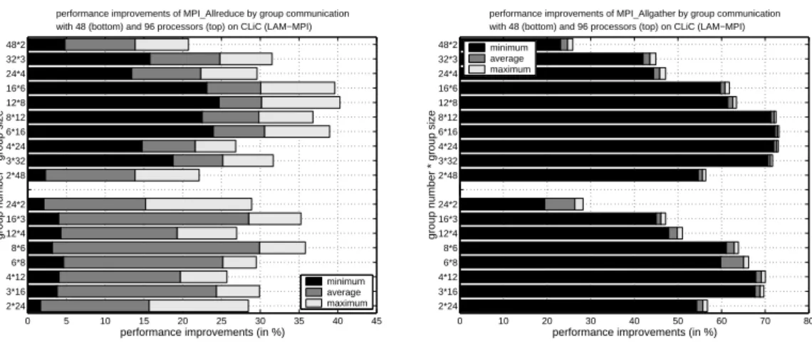
On the CLiC, the orthogonal implementations based on the LAM-MPI library lead to the highest performance improvements for most collective communication operations.

The orthogonal realizations of anMPI Bcast(),MPI Allgather()andMPI Allreduce() op-eration show the most significant performance improvements. All partitions show a con-siderable improvement, but the largest improvements can be obtained when using a layout for which the number of row and column groups are about the same. The MPI Bcast() operation shows significant average improvements of more than 20% for 48 and 40% for 96 processors, respectively, using balanced grid layouts, see Figure 7 (left). The orthogonal implementation of aMPI Allreduce()operation shows average improvements of more than

(9)

[3] [2] [3] [2] [3] [3] [2] [1] [1] [2] [3] [3] [4] [3] 2 P P6 P0 root P1 P4 P3 0 P2 P1 P P4 P6 P5 5 P R1 R2 7 P 3 P 7 P

Figure 6: Illustration of aMPI Bcast() operation with 8 processorsP0, ..., P7 and root processorP0 using a binary tree algorithm. The figure shows a standard implementation using in LAM-MPI (left)

and an orthogonal realization with two groupsR1andR2of 4 processors each (right). The processors

P0 andP4 form the leader group. The number in the squared bracket denotes the message passing

step to distribute the data block. The standard algorithm needs 4 and the orthogonal realization 3 message passing steps to distribute the block of data.

0 10 20 30 40 50 60 2*24 3*16 4*12 6*8 8*6 12*4 16*3 24*2 2*48 3*32 4*24 6*16 8*12 12*8 16*6 24*4 32*3 48*2

performance improvements (in %)

group number * group size

performance improvements of MPI_Bcast by group communication with 48 (bottom) and 96 processors (top) on CLiC (LAM−MPI)

minimum average maximum 0 1 2 3 4 5 6 7 2*24 3*16 4*12 6*8 8*6 12*4 16*3 24*2 2*48 3*32 4*24 6*16 8*12 12*8 16*6 24*4 32*3 48*2

performance improvements of MPI_Gather by group communication with 48 (bottom) and 96 processors (top) on CLiC (LAM−MPI)

minimum average maximum

Figure 7: Performance improvements by group-based realization of MPI Bcast() (left) and

MPI Gather() (right) with 48 and 96 processors on the CLiC (LAM-MPI).

20% for 48 and 30% for 96 processors, respectively, again using balanced group sizes, see Figure 8 (left). The execution time of the MPI Allgather()operation can be dramatically improved by an orthogonal realization, see Figure 8 (right). For some of the group par-titionings, improvements of over 60% for 48 and 70% for 96 processors, respectively, can be obtained. The difference between the minimum and maximum performance enhance-ments are extremely small, which means that this method leads to a reliable improvement for all message sizes.

The main reason for the significant performance improvements of these three collective communication operations achieved by orthogonal realization is the specific implemen-tation of the MPI Bcast() operation in LAM-MPI. The algorithm of the MPI Bcast() operation to distribute the block of data does not exploit the star network topology of the CLiC, but uses a structure describing a tree topology. In general, the orthogonal realiza-tion leads to a better utilizarealiza-tion of the network caused by a more balanced communcarealiza-tion pattern. Figure 6 illustrates the message passing steps of a binary broadcast-tree with 8 processors P0, ..., P7 and demonstrates the benefits of an orthogonal realization.

Both theMPI Allgather()and theMPI Allreduce()operation in the LAM implementation use aMPI Bcast()operation to distribute the block of data to all participating processors. TheMPI Allreduce() operation is composed of anMPI Reduce()and anMPI Bcast() op-eration. First the root processor reduces the blocks of data from all members of the processor group and broadcasts the result buffer to all processors participating in the

(10)

0 5 10 15 20 25 30 35 40 45 2*24 3*16 4*12 6*8 8*6 12*4 16*3 24*2 2*48 3*32 4*24 6*16 8*12 12*8 16*6 24*4 32*3 48*2

performance improvements of MPI_Allreduce by group communication with 48 (bottom) and 96 processors (top) on CLiC (LAM−MPI)

minimum average maximum 0 10 20 30 40 50 60 70 80 2*24 3*16 4*12 6*8 8*6 12*4 16*3 24*2 2*48 3*32 4*24 6*16 8*12 12*8 16*6 24*4 32*3 48*2

performance improvements of MPI_Allgather by group communication with 48 (bottom) and 96 processors (top) on CLiC (LAM−MPI) minimum

average maximum

Figure 8: Performance improvements ofMPI Allreduce()(left) andMPI Allgather (right) by group communication with 48 and 96 processors on the CLiC (LAM-MPI).

communication operation. The message size is constant for both operations. The improve-ments correspond to the performance enhanceimprove-ments of the MPI Bcast() operation, since the preceding MPI Reduce() operation with orthogonal structure leads to a small per-formance degradation. The MPI Allgather() operation is composed of an MPI Gather() and an MPI Bcast() operation. First the root processor collects blocks of data from all members of the processor group and broadcasts the entire message to all processors par-ticipating in the communication operation. The root processor broadcasts a considerably larger message of sizeb·p, whenbdenotes the original message size andpis the number of participating processors. The dramatic improvements are again caused by the execution of the MPI Bcast() operation for the larger message size.

The orthogonal implementation of the MPI Gather() operation shows a small, but per-sistent average performance improvement for all grid layouts of more than 1% for 48 and 2% for 96 processors, respectively, see Figure 7 (right). There are only small variations of the improvements obtained for different layouts, but using the same number of row and column groups again leads to the best average performance. An average performance degradation can be observed for theMPI Scatter()and theMPI Reduce()operation. Only for specific message sizes, a small performance improvement can be obtained, not shown in a figure.

3.2 Orthogonal realization using MPICH on the CLiC

The performance improvements on the CLiC based on the MPICH library are not as significant as with LAM-MPI, but also with MPICH persistent enhancements by an or-thogonal realization can be obtained for some collective communication operations. The orthogonal implementations of the MPI Gather()and MPI Scatter() operations lead to small, but persistent performance enhancements. For the MPI Gather() operation more than 1% for 48 and 2% for 96 processors, respectively, can be obtained using bal-anced grid layouts, see Figure 9 (left). Similar results are shown in Figure 9 (right) for the MPI Scatter() operation. Depending on the message size up to 5% performance en-hancements can be obtained with an optimal grid layout in the best case.

The orthogonal realization of the MPI Allgather() operation leads to very large per-formance improvements for message sizes in the range of 32 KByte and 128 KByte, see Figure 12 (left); for larger message sizes up to 500 KByte slight performance degrada-tion between 1 % and 2 % can be observed. The main reason for the large differences in the improvements depending on the message size are the different protocols used for short and long messages. Both protocols are realized using non-blockingMPI Isend()and

(11)

0 1 2 3 4 5 6 2*24 3*16 4*12 6*8 8*6 12*4 16*3 24*2 2*48 3*32 4*24 6*16 8*12 12*8 16*6 24*4 32*3 48*2

performance improvements of MPI_Gather by group communication with 48 (bottom) and 96 processors (top) on CLiC (MPICH)

performance improvements of MPI_Scatter by group communication with 48 (bottom) and 96 processors (top) on CLiC (MPICH)

Figure 9: Performance improvements by group-based realization of MPI Gather() (left) and

MPI Scatter() (right) with 48 and 96 processors on the CLiC (MPICH).

MPI Irecv() operations. For messages up to 128 KBytes, aneager protocol is used where the receiving processor stores messages that arrive before the corresponding MPI Irecv() operation has been activated in a system buffer. This buffer is allocated each time that such a message arrives. Issuing the MPI Irecv() operation leads to copying the message from the system buffer to the user buffer. For messages that are larger than 128 KBytes, a rendezvous protocol is used that is based on request messages send by the destination processor to the source processor as soon as a receive operation has been issued, so that the message can be directly copied into the user buffer. The reason for the large im-provements for short messages shown in Figure 12 (left) is caused by the fact that the asynchronous standard realization of theMPI Allgather() operation leads to an allocation of a temporary buffer and a succeeding copy operation for a large number of processors whereas the orthogonal group-based realization uses the rendezvous protocol for larger messages in the second communication phase because of an increased message size b·p2.

Slight performance degradations between 1% and 2% can also be observed for the MPI Reduce(), MPI Allreduce() and the MPI Bcast() operations by an orthogonal re-alization which is not shown in a figure.

3.3 Orthogonal realization using LAM-MPI on the dual Xeon

cluster

The Xeon Cluster consists of 16 nodes with two processors per node. The processors participating in a communication operation are assigned to the nodes in a cyclic order to achieve a reasonable utilization of both interconnection networks. For runtime tests with 16 processors all 16 nodes are involved, i.e., processor i uses one physical processor of node i for 0 ≤ i≤ 15. When 32 processors participate in the communication operation, nodei provides the processors i and i+ 16 for 0≤i≤15.

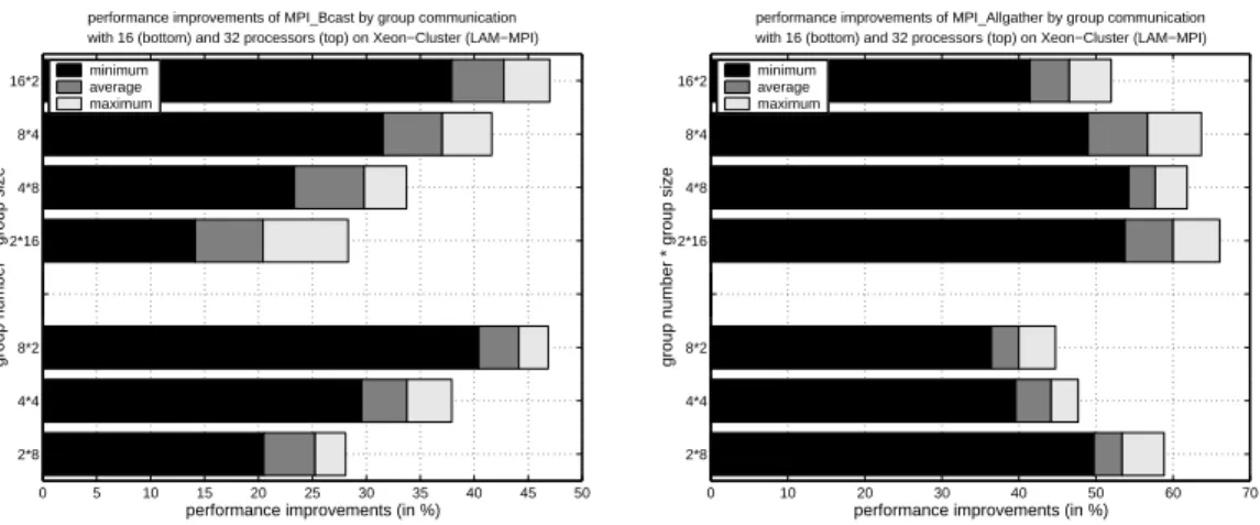
The performance results of the different communication operations are similar to the performance enhancements using LAM-MPI on the CLiC. The main reason is that both platforms use a star network topology, the same interconnection network (fast-Ethernet) and the same realization of communication operation based on the LAM-MPI library. Figure 10 shows as example that for an MPI Bcast() (left) and anMPI Allgather (right) operation similar performance improvement as on the Beowulf cluster can be obtained. Because of the specific processor arrangement of the cluster the performance improve-ments of the various two-dimensional group layouts differ from the performance results on the CLiC, such that a balanced grid layout does not necessarily lead to the best average performance improvement. Concerning performance improvements and grid layouts

(12)

sim-0 5 10 15 20 25 30 35 40 45 50 2*8 4*4 8*2 2*16 4*8 8*4 16*2

performance improvements of MPI_Bcast by group communication with 16 (bottom) and 32 processors (top) on Xeon−Cluster (LAM−MPI) minimum average maximum 0 10 20 30 40 50 60 70 2*8 4*4 8*2 2*16 4*8 8*4 16*2

performance improvements of MPI_Allgather by group communication with 16 (bottom) and 32 processors (top) on Xeon−Cluster (LAM−MPI) minimum

average maximum

Figure 10: Performance improvements by group-based realization of MPI Bcast() (left) and

MPI Allgather() (right) with 16 and 32 processors on the dual Xeon cluster (LAM-MPI).

ilar performance improvements on the CLiC can be observed for the remaining collective MPI communication operations.

3.4 Orthogonal realization using ScaMPI on the Xeon cluster

In general, collective communication operations using the two-dimensional SCI torus are significantly faster than operations using an Ethernet network. Depending on the specific communication operation the SCI interface is by a factor of 100 faster than the Eth-ernet network. Several collective communication operations using ScaMPI on SCI still show performance improvements obtained by orthogonal group realization, see Figure 11 for an MPI Gather (left) and MPI Allgather (right) operation for smaller message sizes. For MPI Scatter similar performance results like for MPI Gather can be observed. For MPI Bcast and the accumulation operations slight performance degradations can be ob-served. The assignment of processors participating in the communication operation to the cluster nodes is done as described in Section 3.3.

0 10 20 30 40 50 60 2*8 4*4 8*2 2*16 4*8 8*4 16*2

performance improvements of MPI_Gather by group communication with 16 (bottom) and 32 processors (top) on Xeon−Cluster (SCALI)

minimum average maximum 0 2 4 6 8 10 12 14 16 18 20 2*8 4*4 8*2 2*16 4*8 8*4 16*2

performance improvements of MPI_Allgather by group communication with 16 (bottom) and 32 processors (top) on Xeon−Cluster (SCALI)

Figure 11: Performance improvements by group-based realization ofMPI Gather()(left) for message

sizes in the range of 560 Byte and 64 KByte and MPI Allgather()(right) for message sizes between

100 KByte and 500 KByte on the Xeon cluster (ScaMPI).

3.5 Orthogonal realization on the Cray T3E-1200

The Cray T3E is a distributed shared memory system in which the nodes are intercon-nected through a bidirectional 3D torus network. The T3E network uses a deterministic,

(13)

0 10 20 30 40 50 60 70 80 90 100 2*24 3*16 4*12 6*8 8*6 12*4 16*3 24*2 2*48 3*32 4*24 6*16 8*12 12*8 16*6 24*4 32*3 48*2

performance improvements of MPI_Allgather by group communication with 48 (bottom) and 96 processors (top) on CLiC (MPICH) minimum average maximum 0 5 10 15 20 25 30 35 40 45 50 2*24 3*16 4*12 6*8 8*6 12*4 16*3 24*2 2*48 3*32 4*24 6*16 8*12 12*8 16*6 24*4 32*3 48*2

performance improvements of MPI_Gather by group communication with 48 (bottom) and 96 processors (top) on Cray T3E−1200

Figure 12: Performance improvements by group-based realization of MPI Allgather() for message

sizes in the range of 32 KByte and 128 KByte on the CLiC (MPICH) (left) and MPI Gather() for

messages sizes between 10 KByte and 500 KByte on the Cray T3E-1200 (right).

dimension-order,k-aryn-cube wormhole routing scheme [17]. Each node contains a table, stored in dedicated hardware, that provides a routing tag for every destination node. In deterministic routing, the path from source to destination is determined by the current node address and the destination node address so that for the same source-destination pair all packets follow the same path. Dimension-order routing is a deterministic rout-ing scheme in which the path is selected that the network is traversed in a predefined monotonic order of the dimensions in the torus. Deadlocks are avoided in deterministic routing by ordering the virtual channels that a message needs to traverse. Dimension-order routing is not optimal for k-ary n-cubes. Because of the wraparound connections, messages may get involved in deadlocks while routing through the shortest paths. In fact, messages being routed along the same dimension (a single dimension forms a ring) may be involved in a deadlock due to a cyclic dependency. A non-minimal deadlock-free deterministic routing algorithm can be developed fork-aryn-cubes by restricting the use of certain edges so as to prevent the formation of cycles [5]. In general, when an algo-rithm restricts message routing to a fixed path, it cannot exploit possible multiple paths between source-destination pairs during congestion.

There considerations show that a standard MPI communication operation does not auto-matically lead to an optimal execution time on the T3E. Furthermore, a rearrangement of a processor set as smaller groups of processors may prevent congestions thus leading to smaller execution times. This will be shown in the following runtime tests. The appli-cation uses the virtual PE number to reference each PE in a partition and has no direct access to logical or physical PE addresses. The hardware is responsible for the conversion of virtual, logical and physical PE numbers.

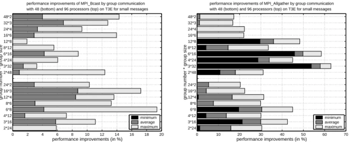
For MPI Bcast() and MPI Allgather() operations, good performance improvements up to 20% can be obtained when using suitable grid layouts for messages in the range of 10 KByte and 500 KByte. The execution times of the orthogonal realizations are quite sensible to the grid layout and the specific message size, i.e. other grid layouts lead to smaller improvements or may even lead to performance degradation. Moreover, there is a large variation of performance improvements especially for large messages where mes-sages of similar size may lead to a significant difference in the performance improvement obtained. This leads to large differences between the minimum and maximum improve-ment. In contrast, smaller message sizes in the range of 10 KByte and 100 KByte lead to persistent average performance improvements for both operations, see Figure 13 for the MPI Bcast() (left) and MPI Allgather() (right) operations.

(14)

0 2 4 6 8 10 12 14 16 18 20 2*24 3*16 4*12 6*8 8*6 12*4 16*3 24*2 2*48 3*32 4*24 6*16 8*12 12*8 16*6 24*4 32*3 48*2

performance improvements of MPI_Bcast by group communication with 48 (bottom) and 96 processors (top) on T3E for small messages

performance improvements of MPI_Allgather by group communication with 48 (bottom) and 96 processors (top) on T3E for small messages

Figure 13: Performance improvements by group communication of MPI Bcast() (left) and

MPI Allgather() (right) for message sizes in the range of 10 KByte and 100 KByte on the Cray T3E-1200.

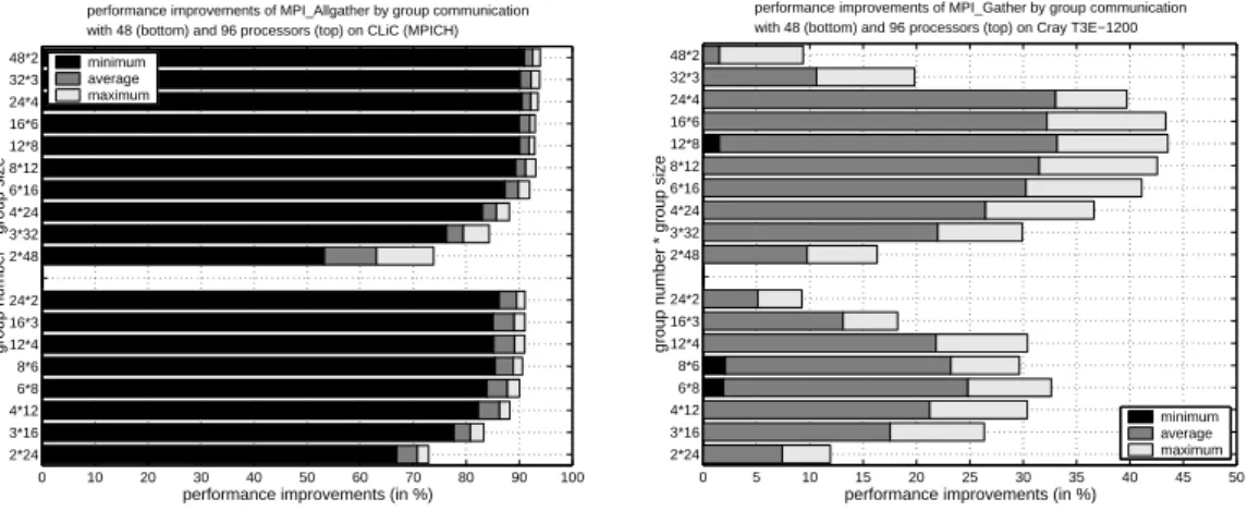
20% for 48 and 30% for 96 processors, respectively, can be obtained, see Figure 12 (right). For small message sizes, a slight performance degradation can sometimes be observed. Therefore there is no minimum improvement shown for most of the layouts in the figure. For message sizes between 128 KBytes and 500 KBytes, the improvements obtained are nearly constant. The runtimes for MPI Gather() operations increase more than linearly with the number p of processors. which is caused by the fact that the root processor becomes a bottleneck when gathering larger messages. This bottleneck is avoided when using orthogonal group communication.

Slight performance degradations between 1% and 2% are obtained for the MPI Scatter(), MPI Reduce()andMPI Allreduce()operations. Neither for smaller nor for larger message sizes performance enhancements can be observed.

3.6 Performance results for hierarchical orthogonal organization

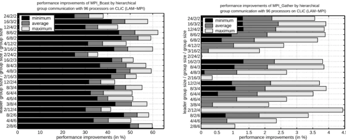
On the CLiC and T3E a sufficiently large number of processors is available to arrange different grid layouts for three communication phases. For up to 96 processors, up to three hierarchical decompositions according to Section 2.2 are useful and we present runtime tests for 96 processors on the CLiC (with LAM-MPI) and on the Cray T3E. In particular, if the original leader group contains 16 or more processors, it is reasonable to decompose this again and the communication is performed in three instead of two phases. Compared to the two-phase realization, a hierarchical realization of theMPI Bcast()andMPI Gather() operation leads to additional and persistent performance improvements on the CLiC and T3E.

Hierarchical realization using LAM-MPI on the CLiC Comparing a

two-dimensional with a three-two-dimensional realization for the MPI Bcast() operation, an ad-ditional performance improvement of up to 15% can be obtained for the CLiC using LAM-MPI. The additional average performance improvement lies above 10% for some of the group partitionings, see Figure 14 (left). The hierarchical realization for the MPI Gather() operation shows no additional performance improvements compared to the two-dimensional realization, see Figure 14 (right). The resulting differences between the minimum and maximum performance improvements are larger for all message sizes than for two-phase realization.

Hierarchical realization on the Cray T3E-1200 For theMPI Bcast()operationall

(15)

0 10 20 30 40 50 60 2/8/6 4/4/6 8/2/6 2/12/4 3/8/4 4/6/4 6/4/4 8/3/4 12/2/4 2/16/3 4/8/3 8/4/3 16/2/3 2/24/2 3/16/2 4/12/2 6/8/2 8/6/2 12/4/2 16/3/2 24/2/2

leader group size / group size / group size

performance improvements of MPI_Bcast by hierarchical group communication with 96 processors on CLiC (LAM−MPI)

minimum average maximum 0 0.5 1 1.5 2 2.5 3 3.5 4 4.5 2/8/6 4/4/6 8/2/6 2/12/4 3/8/4 4/6/4 6/4/4 8/3/4 12/2/4 2/16/3 4/8/3 8/4/3 16/2/3 2/24/2 3/16/2 4/12/2 6/8/2 8/6/2 12/4/2 16/3/2 24/2/2

performance improvements of MPI_Gather by hierarchical group communication with 96 processors on CLiC (LAM−MPI)

Figure 14: Performance improvements by hierarchical group communication of MPI Bcast() (left) andMPI Gather() (right) on the CLiC (LAM-MPI).

0 5 10 15 20 25 30 2/8/6 4/4/6 8/2/6 2/12/4 3/8/4 4/6/4 6/4/4 8/3/4 12/2/4 2/16/3 4/8/3 8/4/3 16/2/3 2/24/2 3/16/2 4/12/2 6/8/2 8/6/2 12/4/2 16/3/2 24/2/2

performance improvements of MPI_Bcast by hierarchical group communication with 96 processors on Cray T3E−1200

minimum average maximum 0 10 20 30 40 50 60 70 80 2/8/6 4/4/6 8/2/6 2/12/4 3/8/4 4/6/4 6/4/4 8/3/4 12/2/4 2/16/3 4/8/3 8/4/3 16/2/3 2/24/2 3/16/2 4/12/2 6/8/2 8/6/2 12/4/2 16/3/2 24/2/2

performance improvements of MPI_Gather by hierarchical group communication with 96 processors on Cray T3E−1200

Figure 15: Performance improvements by hierarchical group communication of MPI Bcast() (left) andMPI Gather() (right) on the Cray T3E-1200.

tests with two communication phases for message sizes up to 500 KByte on the T3E, see Figure 15 (left). For suitable grid layouts average improvements of more than 20% can be obtained. Also for MPI Gather() the hierarchical realization with three communication phases leads to additional performance improvements, see Figure 15 (right). The improve-ments vary depending on the group partitionings. For some of the group partitionings, additional improvements of over 60 % can be obtained.

Hierarchical realization on the Xeon cluster Figure 16 shows performance

en-hancements for four MPI communication operations obtained by a hierarchical orthogo-nal grid layout with three communication phases. Since 32 processors are available three different group layouts (2×8×4, 4×4×2, 8×2×2) are chosen for the Xeon cluster. Figure 16 shows the additional performance improvements for the orthogonal realization of MPI Bcast, MPI Allgather using LAM-MPI (left) and MPI Gather, MPI Scatter us-ing ScaMPI (right). The orthogonal realizations usus-ing ScaMPI are obtained for smaller message sizes in the range of 560 Byte and 64 KByte, see also Section 3.4.

3.7 Grid Selection

For a given machine and a given MPI implementation a different layout of the processor grid lead to the largest performance improvement. A good layout of the processor grid can be selected by performing measurements with different grid layouts and different message sizes for each of the collective communication operations to be optimized.

(16)

0 10 20 30 40 50 60 70 80 2/8/2 4/4/2 8/2/2 2/8/2 4/4/2 8/2/2

performance improvements of MPI_Bcast (top) and MPI_Allgather (bottom) by hierarchical group communication with 32 processors on Xeon cluster (LAM−MPI)

minimum average maximum 0 10 20 30 40 50 60 2/8/2 4/4/2 8/2/2 2/8/2 4/4/2 8/2/2

performance improvements of MPI_Gather (top) and MPI_Scatter (bottom) by hierarchical group communication with 32 processors on Xeon−Cluster (ScaMPI)

Figure 16: Performance improvements by hierarchical group communication of MPI Bcast(),

MPI Allgather() using LAM-MPI (left) and MPI Gather(), MPI Scatter() using ScaMPI (right) on the Xeon cluster. The improvements for orthogonal realizations using ScaMPI (right Figure) are obtained for message sizes between 560 Byte and 64 KByte.

The process of obtaining and analyzing the measurements can be automated such that for each communication operation, a suitable layout is determined that leads to small execution times. This process has to be done only once for each target machine and each MPI implementation and the selected layout can then be used for all communication operations in all application programs. In general, different optimal layouts may result for different communication operations, but our experiments with LAM-MPI, MPICH and Cray-MPI show that using the same number of row and column groups usually leads to good and persistent improvements compared to the standard implementation of the MPI operations.

Also, different grid layouts may lead to the best performance improvement when consider-ing different message sizes for the same communicaton operation. Based on the measured execution times of the communication operation, it is also possible to identify intervals of message sizes such that a different grid layout is selected for a different interval of message sizes, depending on the expected performance improvement. The measured data also shows whether for a specific communication operation and for a specific message size, no performance improvement is expected by an orthogonal realization so that the original MPI implementation can be used. Based on the selection of appropriate grid layouts in two- or multi-dimensional forms an optimized collective communication operation is realized offering the best improvements possible using the orthogonal approach. The result of the analysis step is a realization of the collective communication operations that uses orthogonal realization with a suitable layout whenever it is expected that this leads to a performance improvement compared to the given MPI implememtation.

4 Performance modeling of orthogonal group

struc-tures

In this section, we consider the performance modeling of the orthogonal realization of collective communication operations using runtime functions. Runtime functions have been successfully used to model the execution time of communication operation for various communication libraries [7, 15]. The execution of an MPI Bcast broadcast operation, for

(17)

example, on the CLiC using LAM-MPI 6.3 b2 can be described by the runtime function

tsb(p, b) = (0.0383 + 0.474·10−6·log2(p))·b,

whereb denotes the message size in bytes andp is the number of processors participating in the communication operation. For the performance modeling of orthogonal implemen-tations of collective communication operations we adopt the approach for modeling the execution time of each phase of the orthogonal implementation in isolation. For each phase we use the runtime functions of the monolithic standard MPI communication op-erations from Table 1. The coefficients τ1 and tc can be considered as startup time and

byte-transfer time, respectively, and are determined by applying curve fitting with the least-squares method to measured execution times. For the measurements, message sizes between 10 KBytes and 500 KBytes have been used. In some of the formulas the startup time is very small and can be ignored. In the following, we consider the modeling of orthogonal realizations of some important MPI operations.

MPI Bcast For the broadcast operation the communication time is modeled by adding

the runtime function for the broadcast in the leader group (using the formula from Table 1 with p =p1) and the runtime function for the concurrent broadcast in the row groups

(using the formula from Table 1 withp=p2). The accurate predictions for the concurrent

groups and leader groups show that this approach can be used for all collective MPI communication operations. The good prediction results of the two-phase performance modeling also show that there is no interferences of concurrent communication operations in the second communication phase. A possible interference would lead to a delayed communication time and, thus, would require a different modeling approach.

For the single-broadcast operations, LAM-MPI uses two different internal realizations, one for p ≤ 4 and one for p > 4. If up to 4 processors participate in the broadcast operation, a formula results that depends linearly on p. For more than 4 processors a formula with a logarithmic dependence onpis used, because the broadcast transmissions are based on broadcast trees with logarithmic depth. The corresponding coefficients are given in Table 2.

Figure 17 (left) shows the deviations between measured and predicted execution times for single-broadcast on the CLiC for an orthogonal realization. For different group layouts the deviations are gives separately for the leader group (LG) used in the first phase and the for the concurrent groups (CG) used in the second phase. The bar total shows the accumulated deviation of both communication phases. The figure shows minimum, maximum, and average deviations between measured and predicted runtimes over the entire interval of message sizes. The predictions are quite accurate but not absolutely precise for some groups, because the depth of the broadcast tree remains constant for a specific interval of processor sizes. This means that the communication time increases in stages and the runtime formulas do not model these stages exactly. Figure 17 (right)

operation runtime function

MPI Bcast tsb lin(p, b) = (τ +tc·p)·b tsb log(p, b) = (τ +tc·log2(p))·b

MPI Gather tsc(p, b) =τ1+ (τ2+tc·p)·b

MPI Scatter tga(p, b) =τ1+ (τ2+tc·p)·b

MPI Reduce tacc lin(p, b) = (τ +tc·p)·b

tacc log(p, b) = (τ +tc· blog2(p−1)c)·b

MPI Allreduce tmacc(p, b) =tacc(p, b) +tsb(p, b)

MPI Allgather tmb(p, b) =tga(p, b) +tsb(p, p·b)

(18)

coefficients for broadcast and accumulation

CLiC Xeon cluster

operation formula p τ[µs] tc[µs] p τ[µs] tc[µs]

MPI Bcast tsb lin(p, b) ≤4 -0.085 0.092 - - -tsb log(p, b) >4 0.038s 0.474 >1 -0.0005 0.0042

MPI Reduce tacc lin(p, b) ≤4 -0.103 0.105 - -

-tacc log(p, b) >4 0.141 0.101 >1 0.0116 0.0002

Table 2: Coefficients of the runtime function for MPI Bcast() and MPI Reduce() on the CLiC (LAM-MPI) and on the dual Xeon cluster (ScaMPI).

0 2 4 6 8 10 12 14 16 18 20 LG 02 CG 48total LG 03 CG 32total LG 04 CG 24total LG 06 CG 16total LG 08 CG 12total LG 12 CG 08total LG 16 CG 06total LG 24 CG 04total LG 32 CG 03total LG 48 CG 02total deviation (in %)

leader group (LG), concurrent group (CG)

deviation between measured and predicted runtimes of MPI_Bcast with group communication on CLiC (LAM−MPI)

minimum average maximum 0 0.2 0.4 0.6 0.8 1 1.2 1.4 20 40 60 80 100 120 runtime in seconds processors MPI_Bcast on CLiC with

measurement 100 KB measurement 200 KB measurement 300 KB measurement 400 KB measurement 500 KB prediction 100 KB prediction 200 KB prediction 300 KB prediction 400 KB prediction 500 KB

Figure 17: Deviations between measured and predicted runtimes for 96 processors (left) and

mod-eling (right) of MPI Bcast() on the CLiC.

shows the measured and predicted runtime of the single-broadcast operation as a function of the number of processors for fixed message sizes given in the key.

Figure 18 (left) shows the predictions for the dual Xeon cluster using ScaMPI and in Table 2 the coefficients of the runtime functions are shown.

MPI GatherThe coefficients of the runtime functions for the CLiC are shown in Table

3. The predictions fit the measured runtimes quite accurately, see Figure 19 (left). The approximations are quite accurate for the entire interval of message sizes. The average deviations between measured and predicted runtimes lie clearly below 3 % in most cases. On the T3E, the runtimes ofMPI Gather()operations increase more than linearly with the numberpof processors. This effect might be caused by the fact that the root processor is a bottleneck when gathering larger messages. This observation can be used to obtain good performance improvements by orthogonal realizations. To capture the sharp increases of the runtimes we use different runtime functions for different message sizes. Each increase can be captured by a specific formula, see Table 4. The use of a specific formula depends on the root message size which is the size of the message that the root processor is gathering

coefficients for gather and scatter

CLiC Xeon cluster

operation τ₁(V)[s] τ₂(V)[µs] tc(V)[µs] τ1(V)[s] τ2(V)[µs] tc(V)[µs]

MPI Gather 0.009 -0.0825 0.0929 0.00 -0.0056 0.0040 MPI Scatter 0.00 -0.0730 0.0897 0.00 -0.0032 0.0039

Table 3: Coefficients for runtime function of MPI Gather()andMPI Scatter() on the CLiC (LAM-MPI) and on the dual Xeon cluster (Sca(LAM-MPI).

(19)

runtime functions of gather/scatter operations on Cray T3E-1200 MPI Gather

No. p n[kbyte] runtime function

1 002 - 128 ≤8448 T1(p, b) = (τ2+tc·p)·b

2 017 - 032 >8448 T2(p, b) =τ1+ (τ2+tc·p)·b

3 033 - 128 >8448 T3(p, b) =τ1+ (τ2+tc·p)·b

MPI Scatter T(p, b) = (τ2+tc·p)·b

Table 4: Runtime functions of MPI Gather() andMPI Scatter()on Cray T3E

operation No. τ1(V)[s] τ2(V)[µs] tc(V)[µs]

MPI Gather 1 - -0.00134 0.00308 2 -0.020 0.0157 0.00505 3 -0.036 0.0265 0.00617 MPI Scatter - - 0.0002453 0.00297

Table 5: Coefficients for runtime function ofMPI Gather()and MPI Scatter()on Cray T3E-1200.

from all members of the processor group. Above 8448 KBytes a different runtime formula is used. For the first formula no startup-time is necessary. The values of the coefficients are shown in Table 5. The prediction for the dual Xeon cluster using ScaMPI are given in Figure 18 (right), the coefficients of the runtime function are shown in Table 3. Figure 19 (right) shows the deviations between measured and predicted runtimes on the T3E. The approximations are quite accurate for the entire interval of message sizes. The average deviations of 16 different processor groups (leader and concurrent groups are modeled separately) are clearly below 3 %.

MPI ScatterThe runtime formulas for the predictions of the scatter operations are also

given in Table 4. The values of the coefficients are shown in Table 5. The approximations of the scatter operation show the best results on both systems. On the CLiC the pre-dictions fit the measured runtimes very accurately with an average deviations below 2 % for most processor groups over the entire interval of all message sizes, see also Figure 20 (left). The deviations of the leader group lies below 1 % for almost all group sizes. The deviations between measurements and predictions of the MPI Scatter() operation on the Cray T3E-1200 are shown in Figure 20 (right).

MPI Reduce The modeling of MPI Reduce() operations is performed with the formula

0 2 4 6 8 10 12 LG 02 CG 16 total LG 04 CG 08 total LG 08 CG 04 total LG 16 CG 02 total 32 deviation (in %)

deviation between measured and predicted runtimes of MPI_Bcast with group communication on Xeon cluster (ScaMPI)

minimum average maximum 0 2 4 6 8 10 12 LG 02 CG 16 total LG 04 CG 08 total LG 08 CG 04 total LG 16 CG 02 total 32 deviation (in %)

deviation between measured and predicted runtimes

of MPI_Gather with group communication on Xeon cluster (ScaMPI)

Figure 18: Deviations between measured and predicted runtimes for MPI Bcast() (left) and

(20)

0 2 4 6 8 10 12 14 16 18 20 LG 02 CG 48total LG 03 CG 32total LG 04 CG 24total LG 06 CG 16total LG 08 CG 12total LG 12 CG 08total LG 16 CG 06total LG 24 CG 04total LG 32 CG 03total LG 48 CG 02total deviation (in %)

deviation between measured and predicted runtimes of MPI_Gather with group communication on CLiC (LAM−MPI)

minimum average maximum 0 2 4 6 8 10 12 LG 02 CG 48total LG 03 CG 32total LG 04 CG 24total LG 06 CG 16total LG 08 CG 12total LG 12 CG 08total LG 16 CG 06total LG 24 CG 04total LG 32 CG 03total LG 48 CG 02total deviation (in %)

deviation between measured and predicted runtimes of MPI_Gather with group communication on Cray T3E−1200

Figure 19: Deviations between measured and predicted runtimes for MPI Gather() on the CLiC (left) and Cray T3E-1200 (right) for 96 processors.

0 1 2 3 4 5 6 7 8 LG 02 CG 48total LG 03 CG 32total LG 04 CG 24total LG 06 CG 16total LG 08 CG 12total LG 12 CG 08total LG 16 CG 06total LG 24 CG 04total LG 32 CG 03total LG 48 CG 02total deviation (in %)

deviation between measured and predicted runtimes of MPI_Scatter with group communication on CLiC (LAM−MPI)

minimum average maximum 0 1 2 3 4 5 6 7 8 LG 02 CG 48total LG 03 CG 32total LG 04 CG 24total LG 06 CG 16total LG 08 CG 12total LG 12 CG 08total LG 16 CG 06total LG 24 CG 04total LG 32 CG 03total LG 48 CG 02total deviation (in %)

deviation between measured and predicted runtimes of MPI_Scatter with group communication on Cray T3E−1200

Figure 20: Deviations between measured and predicted runtimes for MPI Scatter() on the CLiC (left) and Cray T3E-1200 (right) for 96 processors.

from Table 1. LAM-MPI uses a different internal realization for p ≤ 4 than for p >

4. The specific values for the coefficients are shown in Table 2 for both cases. The communication time of a reduce operation increases in stages, because the number of time steps to accumulate an array depends on the depth of the reduce tree. A detailed analysis shows that the number of processors can be partitioned into intervals such that for all processor numbers within an interval reduce trees with the same depth are used. The predictions are very accurate and the average deviations between measured and predicted runtimes lie below 3 % for most cases.

MPI Allreduce In LAM-MPI the MPI Allreduce() operation is composed of an

MPI Reduce() and an MPI Bcast() operation. First the root processor reduces the block of data from all members of the processor group und broadcasts the reduced array to all processors participating in the communication operation. The size of the array is con-stant in both phases. Figure 21 shows specific measured and predicted runtimes with fixed message sizes.

MPI Allgather In LAM-MPI the MPI Allgather() operation is composed of an

MPI Gather() and an MPI Bcast() operation. At first the root processor gathers a block of data from each member of the processor group und broadcasts the entire message to all processors participating in the communication operation. The entire message has sizep·b,

(21)

0 0.2 0.4 0.6 0.8 1 1.2 1.4 1.6 12*8 8*12 6*16 4*24 3*32 2*48 runtime in seconds

group number * group size modeling of MPI_Allreduce with concurrent groups on CLiC

measurement 100 KB measurement 200 KB measurement 300 KB measurement 400 KB measurement 500 KB prediction 200KB prediction 200KB prediction 300KB prediction 400KB prediction 500KB 0 5 10 15 20 25 30 35 40 45 50 16*6 8*12 6*16 4*24 3*32 2*48 runtime in seconds

group number * group size modeling of MPI_Allgather with concurrent groups on CLiC

measurement 100 KB measurement 200 KB measurement 300 KB measurement 400 KB measurement 500 KB prediction 100 KB prediction 200 KB prediction 300 KB prediction 400 KB prediction 500 KB

Figure 21: Measured and predicted runtimes for concurrent groups of MPI Allreduce() (left) and

MPI Allgather() (right) on the CLiC.

whenb denotes the original message size andpthe number of involved processors. Figure 21 shows measured and prediced runtimes with fixed message sizes. The predictions fit the measured runtimes quite accurately. The deviations between measured and predicted runtimes lies below 5 % in most cases.

5 Applications and runtime tests

To investigate the efficiency improvement of the approach for entire application programs, we consider parallel implementations of the Jacobi iteration with and without optimized communication in section 5.1. In section 5.2 we consider a complex application program, the parallel Adams methods PAB and PABM to show the performance improvements by concurrent group communication.

5.1 Parallel Jacobi iteration

We consider three different ways to implement the Jacobi iteration in a data parallel way based on a row-wise and a column-wise distribution of the matrix A. For both distributions the computational work for computing the new entries of the next iteration vectorx(k)_{is the same and is equally allocated to the processors. For systems of size}_n_each

processor performspnpq×nmultiplications and about the same number of additions in each

iteration. But because each processor computes different parts and each processor needs the entire new iteration vector x(k) _{in the next iteration step, different communication}

operations are required for the implementations. In the row-wise distribution of A each processor computes pnpq scalar products yielding p

n

pq components of the new iteration

vector. To provide the entire vector to each processor for the next step a multi-broadcast operation (MPI Allgather()) is performed. The execution time of the row-wise Jacobi iteration with p processors and a system size n can be modeled by the formula

Trow(p, n) = 2·

n2

p ·top+Tmb(p, n

p) (1)

where top denotes the time for the execution of an arithmetic operation and Tmb denotes

the runtime formula of the multi-broadcast operation, see Table 1.

In the column-wise distribution of A each processor computes a new vector d of size n. Addition of all those vectors gives the new iteration vector x. Since the vectors d are

(22)

12000 24000 36000 48000 60000 72000 0 5 10 15 20 25 30 35 40 system size n

performance improvement (in %)

performance improvements of Jacobi iteration

by orthogonal group communication with 96 processors on CLiC (LAM−MPI)

row−wise (MPI_Allgather) column−wise (MPI_Allreduce) column−wise (MPI_Bcast) 960 1200 1440 1680 1920 2160 0 5 10 15 20 25 30 35 40 45 50 system size n

performance improvements of Jacobi iteration

by orthogonal group communication with 96 processors on Cray T3E−1200

row−wise (MPI_Allgather) column−wise (MPI_Allreduce) column−wise (MPI_Bcast)

Figure 22: Performance improvements of the Jacobi iteration by orthogonal group communication on the CLiC (LAM-MPI) (left) and for smaller system sizes on the T3E (right).

12000 24000 36000 48000 60000 72000 0 5 10 15 20 25 system size n

performance improvements of Jacobi iteration by orthogonal group communication with 32 processors on Xeon cluster (LAM−MPI)

row−wise (MPI_Allgather) column−wise (MPI_Allreduce) column−wise (MPI_Bcast) 12000 24000 36000 48000 60000 72000 0 5 10 15 20 25 system size n

performance improvements of Jacobi iteration by orthogonal group communication with 32 processors on Xeon cluster (ScaMPI)

row−wise (MPI_Allgather) column−wise (MPI_Gather) column−wise (MPI_Bcast)

Figure 23: Performance improvements of the Jacobi iteration by orthogonal group communication on the Xeon cluster with LAM-MPI (left) and with ScaMPI (right).

located in different address spaces, collective communication is required to perform the addition. There are two possibilities.

Using anMPI Allreduce() and anMPI Allgather()operation results in the execution time

Tcol mb(p, n) = 2·

n2

p ·top+Tmacc(p, n) +Tmb(p, n

p) (2)

where Tmacc denotes the time of an MPI Allreduce() operation.

Using an MPI Reduce() operation and then anMPI Bcast()operation results in the run-time

Tcol sb(p, n) = 2·

n

p ·(n−1)·top+Tacc(p, n) +Tsb(p, n) (3)

where Tacc denotes the runtime formula of an MPI Reduce() operation, see Table 1.

Optimized communication operations Each original collective communication

op-eration can be replaced by the optimized version using concurrent communications on disjoint subsets of processors.

Thus, when using a 2D orthogonal structure the multi-broadcast operationTmb in

Equa-tion (1) and (2) can be replaced by:

Tmb(p, n p) =Tmb(p1, n p) +Tmb(p2, n·p1 p ) (4)

(23)

4*5 4*10 4*15 4*20 4*25 5000 10000 15000 20000 25000 0 2 4 6 8 10 system size modeling of row−wise Jacobi iteration with orthogonal groups on CLiC

processors p=p1*p2

runtime (in sec)

measurement prediction 2*10 2*20 2*30 2*40 2*50 5000 10000 15000 20000 25000 0 2 4 6 8 10 system size modeling of column−wise Jacobi iteration with orthogonal groups on CLiC

processors p=p1*p2

runtime (in sec)

measurement prediction

Figure 24: Modeling of row-wise (left) and column-wise (right) orthogonal realization of Jacobi iteration on the CLiC (LAM-MPI).

where p=p1·p2. The runtime formula of the single-broadcast operation in equation (3)

can be replaced analogously by

Tsb(p, n) =Tsb(p1, n) +Tsb(p2, n). (5)

Figure 22 shows the performance improvements obtained by a 2D orthogonal structure for the CLiC with LAM-MPI (left) and the T3E (right) for the three implementation variants described. Figure 23 shows the improvements for the dual Xeon cluster using LAM-MPI (left) and ScaMPI (right). For the parallel realization using ScaMPI a specific implementation with MPI Gather and MPI Scatter instead MPI Allreduce is shown in Figure 23 (right). The improvements are obtained for a large range of system sizes using balanced grid layouts. Figure 24 compares the performance measurements and predictions obtained by a 2D orthogonal processor structure for the CLiC. The figure shows that the predictions fit the measurements quite good.

5.2 Parallel Adams methods PAB und PABM

Parallel Adams methods are variants of general linear methods for solving ordinary dif-ferential equations (ODEs) y0₍_t_{) =} _f₍_t,_y₍_t_{)) proposed in [19]; the name was chosen due}

to a similarity of the stage equations with classical Adams formulas. General linear methods compute several stage values yκ,i in each time step κ which correspond to

nu-merical approximations of yκ,i = y(tκ+aih) with abscissa vector (ai), i = 1, ..., K, and

stepsize h = tκ − tκ+1. The stage values of one time step are combined in the vector

Yκ = (yκ,1, ...,yκ,K); for an ODE system of size n, this vector has size n·K.

We consider an explicit Parallel Bashforth (PAB) and an implicit parallel Adams-Moulton (PABM) method. The implicit methods use fix-point iteration with the PAB method as predictor. The resulting methods have the advantage that the computations of the parallel stages within each time step are completely independent from each other. Strong data dependencies only occur at the end of each time step. In a data parallel implementation of the PAB method, the stage values are computed one after another with all processors available. The computation includes K function evaluations of function f, the computation of new stage values, and K multi-broadcast operations. The resulting communication overhead within one time step is given by

(24)

8 16 32 48 64 96 128 8 16 32 48 64 96 128 8 16 32 48 64 96 128 0 10 20 30 40 50 60 70 80 90 processors

time per step in seconds

PABM−method for K=8 on CLiC (MPICH)

n=80000 n=180000 n=320000

data parallel data parallel orthogonal task parallel task parallel orthogonal

4 8 16 24 32 4 8 16 24 32 4 8 16 24 32 0 2 4 6 8 10 12 processors

time per step in seconds

PABM−method for K=8 on Xeon cluster (ScaMPI)

n=80000 n=180000 n=320000

data parallel data parallel orthogonal task parallel task parallel orthogonal

Figure 25: Runtime per time step of the PABM-method forK = 8by orthogonal group communi-cation on the CLiC using MPICH (left) and on the dual Xeon cluster using ScaMPI (right).

5000 20000 45000 80000 180000 0 10 20 30 40 50 60 70 80 90 100 system size n

group number / group size performance improvements of PAB−method

2/48 3/32 4/24 6/16 8/12 12/8 16/6 24/4 32/3 48/2 5000 20000 45000 80000 180000 0 10 20 30 40 50 60 70 80 90 100 system size n

group number / group size performance improvements of PABM−method

2/48 3/32 4/24 6/16 8/12 12/8 16/6 24/4 32/3 48/2

Figure 26: Performance improvements of the data parallel PAB-method (left) and PABM-method (right) by orthogonal group communication on the CLiC (LAM-MPI).

The computation time of one time step is given by

TP AB(n, p) = K·(n/p·Teval(f) + (2K+ 1)·n/p·top)

where Teval(f) is the time for evaluating one component off.

The PABM method uses the PAB method as predictor and uses the PAM method for a fixed number I of iterations in the corrector step. This implementation strategy results in the following communication overhead within one time step:

CP ABM(n, p) =K ·I·Tmb(p, n/p).

The computation time is:

TP ABM(n, p) =K·I·n/p·Teval(f) +K ·(2K+ 1)·n/p·top+K·I·3·n/p·top.

Figure 25 (left) shows the runtime per step of the PABM-method with and without orthogonal structure on the CLiC based on the MPICH library for different implemen-tations. As application, an ODE system has been used that results from the spatial discretization of a reaction-diffusion equation. This is a sparse ODE system, i.e., the evaluation time of one component of f is constant. We consider a data parallel, an or-thogonal data parallel, a task parallel and an oror-thogonal task parallel implementation

MPI Implementation Analysis - A Practical Approach to Network Marketing

Optimizing MPI Collective Communication by

Orthogonal Structures

Matthias K¨

uhnemann

Thomas Rauber

Gudula R¨

unger

Contents

1

Introduction

2

Orthogonal structures for realizing communication

operations

2.1

Realization using a two-dimensional processor grid

P

C

C

R

P

P

P

P

R

P

R

2.2

Realization using a hierarchical processor grid

3

MPI Performance results in isolation

3.1

Orthogonal realization using LAM-MPI on the CLiC

3.2

Orthogonal realization using MPICH on the CLiC

3.3

Orthogonal realization using LAM-MPI on the dual Xeon

cluster

3.4

Orthogonal realization using ScaMPI on the Xeon cluster

3.5

Orthogonal realization on the Cray T3E-1200

3.6

Performance results for hierarchical orthogonal organization

3.7

Grid Selection

4

Performance modeling of orthogonal group

struc-tures

5

Applications and runtime tests

5.1

Parallel Jacobi iteration

5.2

Parallel Adams methods PAB und PABM