Logitboost of Simple Bayesian Classifier
S. B. Kotsiantis and P. E. Pintelas {sotos, pintelas}@math.upatras.gr
Educational Software Development Laboratory Department of Mathematics
University of Patras, Hellas
Keywords: supervised machine learning, predictive data mining
Received: November 30, 2004
The ensembles of simple Bayesian classifiers have traditionally not been a focus of research. The reason is that simple Bayes is an extremely stable learning algorithm and most ensemble techniques such as bagging is mainly variance reduction techniques, thus not being able to benefit from its integration. However, simple Bayes can be effectively used in ensemble techniques, which perform also bias reduction, such as Logitboost. However, Logitboost requires a regression algorithm for base learner. For this reason, we slightly modify simple Bayesian classifier in order to be able to run as a regression method. Finally, we performed a large-scale comparison on 27 standard benchmark datasets with other state-of-the-art algorithms and ensembles using the simple Bayesian algorithm as base learner and the proposed technique was more accurate in most cases.
Povzetek: Preprosti Bayesov klasifikator je uporabljen v varianti Logiboost algoritma.
1
Introduction
The assumption of independence of simple Bayesian classifier is clearly almost always wrong. However, a large-scale comparison of simple Bayesian classifier with state-of-the-art algorithms for decision tree induction and instance-based learning on standard benchmark datasets found that simple Bayesian classifier sometimes is superior to each of the other learning schemes even on datasets with substantial feature dependencies [5]. An explanation why simple Bayesian method remains competitive, even though it provides very poor estimates of the true underlying probabilities can be found in [9]. Although simple Bayesian method remains competitive, the ensembles of simple Bayesian classifiers have not been a focus of research. The explanation is that simple Bayes is a very stable learning algorithm and most ensemble techniques such as bagging is mainly variance reduction techniques, thus not being able to benefit from its combination.
In this study, we combine simple Bayesian method with Logitboost [10], which is a bias reduction technique. As it is well known, Logitboost requires a regression algorithm for base learner. For this reason, we slightly modify simple Bayesian classifier in order to be able to run as a regression method. Finally, we performed a large-scale comparison with other state-of-the-art algorithms and ensembles on 27 standard benchmark datasets and the proposed technique was more accurate in most cases.
Description of some of the attempts that have been tried to improve the performance of simple Bayesian classifier using ensembles techniques is given in section 2. Section 3 discusses the proposed method. Experiment results in a number of data sets are presented in section 4, while brief
summary with further research topics are given in Section 5.
2
Ensembles of simple Bayesian
classifiers
Lately in the area of ML the concept of combining classifiers is proposed as a new direction for the improvement of the performance of individual classifiers. In [1], the researchers built an ensemble of simple Bayes classifiers using bagging [3] and boosting procedures [7]. They concluded that bagging did not manage to improve the results of simple Bayes classifier. The researchers also reported that there was a problem with boosting which was the robustness to noise. This is expected because noisy examples tend to be misclassified, and the weight will be increased for these examples.
Other researchers presented Naive Bayes tree learner, called NBTree [11] that combines Naive Bayesian classification and decision tree learning. It uses a tree structure to split the instance space into sub-spaces defined by the path of the tree. A Naive Bayesian classifier is then generated in each sub-space. Each leaf of the Naive Bayesian tree contains a local Naive Bayesian classifier. As in many other learning algorithms that are based on tree structure, NBTree suffers from the small disjunct problem. To tackle this problem, other researchers [24] applied lazy learning techniques to Bayesian tree in-duction and presented the resulting lazy Bayesian rule learning algorithm LBR. LBR constructs a Bayesian rule specifically for an input test example and uses this rule to predict the class label of the example. Another way that has been examined for generation of ensemble of simple Bayesian classifiers is by using different feature subsets randomly and taking a vote of the predictions of each classifier that uses different feature subset [21].
Melville and Mooney [14] present another meta-learner (DECORATE, Diverse En-semble Creation by Oppositional Relabeling of Artificial Training Examples) that uses a learner to build a diverse committee. This is accomplished by adding different randomly constructed examples to the training set when building new committee members. These artificially constructed examples are given category labels that disagree with the current decision of the committee, thereby directly increasing diversity when a new classifier is trained on the augmented data and added to the committee.
Finally, AODE classification algorithm [22] averages all models from a restricted class of one-dependence classifiers, the class of all such classifiers that have all other attributes depend on a common attribute and the class. The authors’ experiments suggest that the resulting classifiers have substantially lower bias than Naive Bayes at the cost of a very small increase in variance.
3
Presented Algorithm
As we have also mentioned, Naive Bayes can be effectively used in ensemble techniques that perform bias reduction, such as Logitboost. However, Logitboost requires a regression algorithm for base learner. For this reason, we slightly modify simple Bayesian classifier so as to be able to run as a regression method.
Naive Bayes classifier is the simplest form of Bayesian network [5] since it captures the assumption that every feature is independent from the rest of the features, given the state of the class feature. Naive Bayes classifiers operate on data sets where each example x consists of feature values <a1, a2 ... ai> and the target function f(x) can take on any value from a pre-defined finite set V=(v1, v2 ... vj). Classifying unseen examples involves calculating the most probable target value vmax and is defined as:
(
|
,
,...,
)
.
max
1 2max j i
V
v
P
v
a
a
a
v
j∈
=
Using Bayes theorem vmax can be rewritten as:
(
,
,...,
|
) ( )
.
max
1 2max i j j
V
v
P
a
a
a
v
P
v
v
j∈
=
Under the assumption that features values are conditionally independent given the target value. The formula used by the Naive Bayes classifier is:
( ) ( )
∏
∈
=
i
j i j
V
v
P
v
P
a
v
v
j
|
max
max
where V is the target output of the classifier and P(ai|vj) and P(vi) can be calculated based on their frequency in the training data.
Thus, Naive Bayes assigns a probability to every possible value in the target range. The resulting distribution is then condensed into a single prediction. In categorical problems, the optimal prediction under zero-one loss is the most likely value—the mode of the underlying distribution. However, in numeric problems the optimal prediction is either the mean or the median, depending on the loss function. These two statistics are far more sensitive to the underlying distribution than the most likely value: they almost always change when the underlying distribution changes, even by a small amount. For this reason NB is not as stable in regression as in classification problems. Some researchers have previously applied Naive Bayes to regression problems [6].
Generally, mapping regression into classification is a kind of pre-processing technique that enables us to use classification algorithms on regression problems. The use of the algorithm involves two main steps. First there is the creation of a data set with discrete classes. This step involves looking at the original continuous class values and dividing them into a series of intervals. Each of these intervals will be a discrete class. Every example whose output variable value lies within an interval will be assigned the respective discrete class. The second step consists on reversing the discretisation process after the learning phase takes place. This will enable us to make numeric predictions from our learned model.
One of the most well known techniques for discritization of numerical attributes is the Equal Width intervals (EW). This strategy creates a set of N intervals with the same number of elements. To better illustrate this strategy we show how they group the set of values {1,3,6,7,8,9.5,10,11} assuming that we want to partition them into three intervals (N=3). Using equal width we get [1 .. 4.33], {4.33 .. 7.66] and [7.66 .. 11] containing the values {1,3}, {6,7} and {8,9.5,10,11}.
For the proposed algorithm, we discretized the target value into a set of 10 equal-width intervals, and applied Naive Bayes for classification to the discretized data. At test time, the predicted value is the weighted average of each bin’s value, using the classifiers probabilistic class memberships as weights.
)
(
)
(
1x
f
c
x
F
m M m m∑
==
where the cm are constants to be determined and fm are basis functions.
If we assume that F(x) is the mapping that we seek to fit as our strong aggregate hypothesis, and f(x) are our weak hypotheses, then it can be shown that the two-class Adaboost algorithm is fitting such a model by minimizing the criterion:
)
(
)
(
F
E
e
yF(x)J
=
−where y is the true class label in {-1,1}. Logitboost minimises this criterion by using Newton-like steps to fit an additive logistic regression model to directly optimise the binomial log-likelihood:
)
1
log(
+
e
−2yF(x)−
Finally, the proposed algorithm (LogitBoostNB) is summarized in (Figure 1), where pj are the class probabilities returned by NB, N is the number of the examples of the dataset and J is the number of classes of the dataset.
Step 1: Initialization
• Start with weights wi,j=1/N, i=1,…,N, j=1,…,J, Fj(x)=0 and pj=1/J
∀
j
• Discretize the target value into a set of 10 equal-width intervals
Step 2: LogitBoost iterations: for m=1,2,...,10 repeat: A. Fitting the NB learner For j=1,...,J
• Compute working responses and weights for the jth class
))
(
1
)(
(
)
(
* , . i j i j i j j i j ix
p
x
p
x
p
y
z
−
−
=
where y* the current response
))
(
1
)(
(
.j j i j i
i
p
x
p
x
w
=
−
• Fit the function fmj(x) by a weighted least squares regression of zij to xi with weights wij
B. Set
∑
=
−
−
←
J k mk mjmj
f
x
J
x
f
J
J
x
f
1))
(
1
)
(
(
1
)
(
and)
(
)
(
)
(
x
F
x
f
x
F
j←
j+
mjC. Set
∑
==
J k x F x F j k je
e
x
p
1 ) ( ) ()
(
, enforcing the condition∑
==
J k kx
F
10
)
(
Step 3: Output the classifier argmaxjFj(x) Figure 1: The proposed algorithm
In the following section, we present the experiments. It must be mentioned that the comparisons of the proposed algorithm are separated in three phases: a) with the other attempts that have tried to improve the accuracy of the simple Bayes algorithm, b) with other state-of-the-art algorithms and c) with other well-known ensembles.
4
Comparisons and Results
For the purpose of our study, we used 27 well-known datasets from many domains mainly from the UCI repository [2]. These data sets were hand selected so as to come from real-world problems and to vary in characteristics. Thus, we have used data sets from the domains of: pattern recognition (iris, zoo), image recognition (ionosphere, sonar), medical diagnosis (breast-cancer, breast-w, colic, diabetes, heart-c, heart-h, heart-statlog, hepatitis, lymphotherapy, primary-tumor) commodity trading (autos, credit-g) computer games (monk1, monk2, monk3), various control applications (balance) and prediction of student dropout (student) [12].
In Table 1, there is a brief description of these data sets.
Table 1: Description of the data sets Datasets Instances Categ.
features
Numer.
features Classes autos 205 10 15 6 badge 294 4 7 2
balanceScale 625 0 4 3
breast-cancer 286 9 0 2
breast-w 699 0 9 2
colic 368 15 7 2
credit-g 1000 13 7 2
diabetes 768 0 8 2
haberman 306 0 3 2
heart-c 303 7 6 5
heart-h 294 7 6 5
heart-statlog 270 0 13 2
hepatitis 155 13 6 2
ionosphere 351 34 0 2
iris 150 0 4 3 labor 57 8 8 2
lymph/rapy 148 15 3 4
monk1 124 6 0 2 monk2 169 6 0 2 monk3 122 6 0 2
relation 2201 3 0 2
sonar 208 0 60 2
student 344 11 0 2
vechicle 846 0 18 4
vote 435 16 0 2 wine 178 0 13 3
In order to calculate the classifiers’ accuracy, the whole training set was divided into ten mutually exclusive and equal-sized subsets and for each subset the classifier was trained on the union of all of the other subsets. Then, cross validation was run 10 times for each algorithm and the average value of the 10-cross validations was calculated. It must be mentioned that we used for the most of the algorithms the free available source code by the book [23].
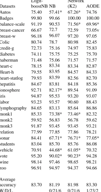
In Table 2, we represent with “v” that the proposed LogitBoostNB algorithm looses from the specific algorithm. That is, the specific algorithm performed statistically better than LogitBoostNB according to t-test with p<0.05. Furthermore, in Table 2, “*” indicates that LogitBoostNB performed statistically better than the specific classifier according to t-test with p<0.05. In all the other cases, there is no significant statistical difference between the results (Draws). In the last rows of the Table 2 one can see the aggregated results in the form (a/b/c). In this notation “a” means that the proposed algorithm is significantly less accurate than the compared algorithm in a out of 27 datasets, “c” means that the proposed algorithm is significantly more accurate than the compared algorithm in c out of 27 datasets, while in the remaining cases (b), there is no significant statistical difference between the results. We also present the average accuracy of all the examined algorithms in all tested datasets.
The proposed algorithm is significantly more accurate than simple Bayes (NB) in 6 out of the 27 datasets, while it has not significantly higher error rates than simple Bayes in none dataset (see Table 2). Moreover, the proposed algorithm is significantly more accurate than AODE [22] in 2 out of the 27 datasets, while it has significantly higher error rates than AODE in one dataset.
We also compared the proposed algorithm with a Bayesian network classifier that is an extension of the simple Bayesian classifier. Several algorithms have been proposed in the last decade for inductive learning of Bayesian networks. Our experiments are based on the Bayesian scoring approach first used in K2 [4]. K2 proceeds by initially assuming that a node has no parents, and then adding incrementally that parent whose addition most increases the probability of the resulting network. Parents are added greedily to a node until the addition of no one parent can increase the structure probability. The proposed algorithm is significantly more accurate than Bayesian Network (K2) in 6 out of the 27 datasets, while it has not significantly higher error rates than simple Bayes in none dataset.
Table 2: Comparing the proposed algorithm with other Bayesian classifiers
Datasets
Logit-boostNB NB
Bayesian Network
(K2) AODE Autos 75.40 57.41* 67.26* 74.76 Badges 99.80 99.66 100.00 100.00 balance-scale 91.19 90.53 71.56* 69.96* breast-cancer 66.67 72.7 72.59 73.05v breast-w 96.18 96.07 97.20 97.05 Colic 80.74 78.7 80.98 82.45 credit-g 72.73 75.16 74.97 75.83 diabetes 74.11 75.75 75.25 75.70 haberman 71.48 75.06 71.57 71.57 heart-c 78.15 83.34 83.34 82.87 Heart-h 79.55 83.95 84.57 84.33 heart-statlog 79.93 83.59 82.56 82.70 hepatitis 84.67 83.81 84.18 85.36 ionosphere 92.71 82.17* 89.54 91.09 iris 94.87 95.53 93.20 93.07 labor 93.23 93.57 90.60 88.43 lymphography 84.65 83.13 85.64 86.86 monk1 85.33 73.38* 73.46* 82.32 monk2 59.92 56.83 56.78 59.62 monk3 91.87 93.45 93.45 93.21 relation 77.99 77.85 77.86 78.21 sonar 84.41 67.71* 76.71* 77.05* students 83.04 85.70 85.76 86.08 vehicle 70.91 44.68* 61.05* 70.32 vote 95.20 90.02* 90.23* 94.28 wine 98.14 97.46 98.65 98.21 zoo 96.91 94.97 94.37 94.66 Average
accuracy 83.70 81.19 81.98 83.30
W/D/L 0/21/6 0/21/6 1/23/2
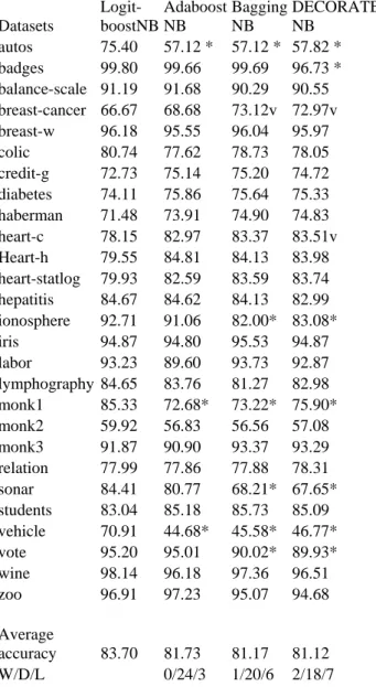
Table 3: Comparing the proposed algorithm with well known ensembles of NB
Datasets
Logit-boostNB
Adaboost NB
Bagging NB
DECORATE NB
autos 75.40 57.12 * 57.12 * 57.82 * badges 99.80 99.66 99.69 96.73 * balance-scale 91.19 91.68 90.29 90.55 breast-cancer 66.67 68.68 73.12v 72.97v breast-w 96.18 95.55 96.04 95.97 colic 80.74 77.62 78.73 78.05 credit-g 72.73 75.14 75.20 74.72 diabetes 74.11 75.86 75.64 75.33 haberman 71.48 73.91 74.90 74.83 heart-c 78.15 82.97 83.37 83.51v Heart-h 79.55 84.81 84.13 83.98 heart-statlog 79.93 82.59 83.59 83.74 hepatitis 84.67 84.62 84.13 82.99 ionosphere 92.71 91.06 82.00* 83.08*
iris 94.87 94.80 95.53 94.87
labor 93.23 89.60 93.73 92.87 lymphography 84.65 83.76 81.27 82.98
monk1 85.33 72.68* 73.22* 75.90* monk2 59.92 56.83 56.56 57.08 monk3 91.87 90.90 93.37 93.29 relation 77.99 77.86 77.88 78.31 sonar 84.41 80.77 68.21* 67.65* students 83.04 85.18 85.73 85.09 vehicle 70.91 44.68* 45.58* 46.77* vote 95.20 95.01 90.02* 89.93* wine 98.14 96.18 97.36 96.51
zoo 96.91 97.23 95.07 94.68
Average
accuracy 83.70 81.73 81.17 81.12 W/D/L 0/24/3 1/20/6 2/18/7 In Table 4, one can see the comparisons of the proposed algorithm with other more sophisticated ensembles of the simple Bayes algorithm. The proposed algorithm is significantly more precise than BoostFSNB algorithm [13] in 4 datasets, whilst it has not significantly higher error rates in any dataset. In addition, the proposed algorithm is significantly more accurate than NBTree [11] algorithm in 1 out of the 27 datasets, whereas it has significantly higher error rates in none dataset.
Furthermore, the proposed algorithm is significantly more precise than LBR [24] algorithm in 2 out of the 27 datasets, while it has significantly higher error rates in one dataset.
In brief, we managed to improve the performance of the simple Bayes Classifier obtaining better accuracy than other well known methods that have tried to improve the performance of the simple Bayes algorithm.
Table 4: Comparing the proposed algorithm with other well known ensembles of NB
Datasets
Logit-boostNB BoostFSNB NBTree LBR
autos 75.40 76.33 77.18 74.04
badges 99.80 100.00 100.00 100.00 balance-scale 91.19 81.98* 75.83* 72.17* breast-cancer 66.67 72.07 70.99 72.35 Breast-w 96.18 96.05 95.97 97.23
colic 80.74 82.35 81.88 82.33
credit-g 72.73 71.36 74.07 74.90 Diabetes 74.11 75.10 75.18 75.38 haberman 71.48 73.08 71.97 71.57 heart-c 78.15 82.15 80.60 83.54 heart-h 79.55 83.61 81.33 84.54 heart-statlog 79.93 82.26 80.59 82.59 Hepatitis 84.67 84.81 81.36 84.97 ionosphere 92.71 91.86 89.49 89.92
iris 94.87 93.47 93.53 93.20
labor 93.23 88.03 91.70 87.50
lymphography 84.65 82.99 80.89 85.45 monk1 85.33 69.67* 91.78 94.91v monk2 59.92 61.43 63.72 60.40 monk3 91.87 92.88 92.94 93.45 relation 77.99 77.23 78.00 78.31 sonar 84.41 77.95* 77.16 76.47* students 83.04 86.20 84.62 85.38 vehicle 70.91 62.14* 71.03 69.43
vote 95.20 95.26 95.03 94.11
wine 98.14 96.84 96.57 98.71
zoo 96.91 95.75 94.55 93.21
Average
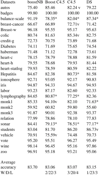
accuracy 83.70 82.70 83.26 83.56 W/D/L 0/23/4 0/26/1 1/26/2 Finally, we compare the performance of the proposed technique with bagging decision trees and boosting decision trees that have been proved to be very successful for many machine-learning problems [18]. Similarly with the proposed algorithm, Quinlan [18] used 10 iterations for bagging and boosting C4.5 algorithm [17]. We also compare the proposed algorithm with Logitboost Decision Stump, which was the base learner used by the authors who proposed Logitboost [10]. In the last rows of the Table 5 one can see the aggregated results.
DS algorithm (using 25 classifiers) in 3 out of the 27 datasets, while in 1 dataset, the proposed algorithm has significantly higher error rate.
Table 5: Comparing the proposed algorithm with well known ensembles
Datasets
Logit-boostNB Boost C4.5
Bagging C4.5
Logit-boost DS
autos 75.40 85.46 82.24 v 79.22 badges 99.80 100.00 100.00 100.00
balance-scale 91.19 78.35* 82.04* 87.34* breast-cancer 66.67 66.89 72.71v 71.42 Breast-w 96.18 95.55 95.17 95.63 colic 80.74 81.63 85.34v 82.75 credit-g 72.73 70.75 73.89 71.68 Diabetes 74.11 71.69 75.65 74.54 haberman 71.48 71.12 72.78 73.61 heart-c 78.15 78.79 78.88 81.59 heart-h 79.55 78.68 79.93 81.44 heart-statlog 79.93 78.59 80.59 82.22 Hepatitis 84.67 82.38 80.73* 81.58 ionosphere 92.71 93.05 92.17 90.83
iris 94.87 94.33 94.67 94.93
labor 93.23 87.17 82.60 92.33
lymphography 84.65 80.87* 77.25* 82.36 monk1 85.33 94.10v 82.10 71.63* monk2 59.92 60.82 59.80 55.60 monk3 91.87 90.01 92.38 93.37 relation 77.99 78.86 78.10 77.83 sonar 84.41 79.13* 78.51* 77.17* students 83.04 81.70 86.20 86.73v vehicle 70.91 75.59v 74.48 70.73
vote 95.20 95.51 96.27 95.49
wine 98.14 96.45 95.16 97.86
zoo 96.91 95.18 93.21 95.06
Average
accuracy 83.70 83.06 83.07 83.15 W/D/L 2/22/3 3/20/4 1/23/3 To sum up, the proposed technique has better performance than all the tested algorithms.
5
Conclusion
Ideally, we would like to be able to identify or design the single best learning algorithm to be used in all situations. However, both experimental results [15] and theoretical work [16] indicate that this is not possible. The simple Bayes classifier has much broader applicability than previously thought. Besides its high classification accuracy, it also has advantages in terms of simplicity, learning speed, classification speed and storage space. In this work, we managed to improve the performance of the simple Bayesian Classifier. We combined simple Bayesian method with Logitboost [10]. However, as it is
well known, Logitboost requires a regression algorithm for base learner. For this reason, we slightly modified simple Bayesian classifier in order to run as a regression method. We performed a large-scale comparison with other attempts that have tried to improve the accuracy of the simple Bayes algorithm as well as other state-of-the-art algorithms and ensembles on 27 standard benchmark datasets and the proposed technique had better accuracy in most cases.
In future research it would be interesting to find a more sophisticated algorithm for choosing the number of intervals, for the application of Naive Bayes to the discretized data. How many intervals should be generated? Depending on the application, the trend of the error of the class mean or median for a variable number of classes can be observed. Too few intervals would imply an easier classification problem, but put an unacceptable limit on the potential performance; too many intervals might make the classification problem too difficult.
References
[1] E. Bauer, and R. Kohavi. An empirical comparison of voting classification algorithms: Bagging, boosting, and variants, Machine Learning, 36 (1999): 105–139.
[2] C. L. Blake and C. J. Merz, UCI Repository of machine
learning databases [http://www.ics.uci.edu/~mlearn/MLRepository.html].
Irvine, CA: University of California, Department of Information and Computer Science (1998).
[3] L. Breiman, Bagging Predictors. Machine Learning, 24 (1996): 123-140.
[4] G.F. Cooper and E. Herskovits (1992). A Bayesian Method for the Induction of Probabilistic Networks from Data. Machine Learning, Vol. 9, pp 309-347. Kluwer Academic Publishers, Boston.
[5] P. Domingos and M. Pazzani, On the optimality of the simple Bayesian classifier under zero-one loss, Machine Learning, 29(1997): 103-130.
[6] E. Frank, Trigg L., Holmes G. and Witten I.H. (2000), Technical Note: Naive Bayes for regression, Machine Learning, 41(1) 5-26, October.
[7] Y. Freund and R. E. Schapire, Experiments with a New Boosting Algorithm, In Proceedings of ICML’96, 148-156.
[8] J. H. Friedman, On bias, variance, 0/1-loss and curse-of-dimensionality. Data Mining and Knowledge Discovery, 1(1997): 55-77.
[9] N. Friedman, D. Geiger and M. Goldszmidt, Bayesian network classifiers. Machine Learning, 29(1997): 131-163. [10]J. Friedman, T. Hastie and R. Tibshirani, Additive Logistic Regression: a Statistical View of Boosting, The Annals of Statistics, 28: 337-374, 2000.
[11]R. Kohavi. Scaling up the accuracy of Naive-Bayes classifiers: A decision-tree hybrid. Proceedings of the second International Conference on Knowledge Discovery and Data Mining. Menlo Park, CA: The AAAI Press. 1996. pp. 202-207
[12]S. Kotsiantis, C. Pierrakeas and P. Pintelas, Preventing student dropout in distance learning systems using machine learning techniques, Lecture Notes in Artificial Intelligence, Springer-Verlag Vol 2774, pp 267-274. [13]S. Kotsiantis, P. Pintelas, Increasing the Classification
Artificial Intelligence, Springer-Verlag Vol 3192, pp. 198-207.
[14]P. Melville, and R. Mooney (2003), Constructing Diverse Classifier Ensembles using Artificial Training Examples, Proceedings of the IJCAI-2003, pp.505-510, Acapulco, Mexico, August 2003
[15]D. Michie, D. Spiegelhalter and C. Taylor, Machine Learning, Neural and Statistical Classification, Ellis Horwood, 1994.
[16]T. Mitchell, Machine Learning, McGraw Hill, 1997. [17]J.Quinlan, C4.5: Programs for machine learning. Morgan
Kaufmann, San Francisco, 1993.
[18]J. R. Quinlan, Bagging, boosting, and C4.5. In Proceedings of the Thirteenth National Conference on Artificial Intelligence (1996), 725–730.
[19]G. Ridgeway, D. Madigan and T. Richardson, Interpretable boosted Naive Bayes classification. In Proceedings of the Fourth International Conference on Knowledge Discovery and Data Mining, Menlo Park (1998): 101-104.
[20]K. Ting and Z. Zheng,. Improving the Performance of Boosting for Naive Bayesian Classification, N. Zhong and L. Zhou (Eds.): PAKDD’99, LNAI 1574, pp. 296-305, 1999.
[21]A. Tsymbal, S. Puuronen and D. Patterson, Feature Selection for Ensembles of Simple Bayesian Classifiers, In Proceedings of ISMIS (2002): 592-600, Lyon, June 27-29. [22]G. Webb, J. Boughton & Z. Wang (2004). Not So Naive
Bayes, To be published in Machine learning journal. [23]I. Witten and E. Frank, Data Mining: Practical Machine
Learning Tools and Techniques with Java Implementations. Morgan Kaufmann, San Mateo, 2000. [24]Z. Zheng, and G.I. Webb, Lazy learning of Bayesian rules.