Determination of Minimum Miscibility Pressure in Gas Injection Process by
Using ANN with Various Mixing Rules
M.R. Akbari*, N. Kasiri
Computer Aided Process Engineering Center, CAPE,
Chem. Eng Dept., Iran University of Sci. & Tech., IUST,
Narmak, Tehran, Iran, 009821-77490416,
[email protected]
[email protected]
Abstract
Miscible gas injection is one of the most effective enhanced oil recovery techniques and minimum miscibility pressure (MMP) is an important parameter in miscible gas injection processes. Accurate determination of this parameter is critical for an adequate design of injection equipments project investment prospect. The purpose of this paper is to develop a new universal artificial neural network (U-ANN) model to predict the minimum miscibility pressure of CO2 and hydrocarbon gas flooding. Different MMP correlations and models have been proposed
regarding the type of injection gas and the mechanism of miscibility, respectively based on mathematical and thermodynamic calculations. Almost all the correlations proposed in the literature either represent condensing
/vaporizing mechanisms or give reasonable results only in a limited range of data they are based on. A new model is introduced by taking into consideration both condensing and vaporizing mechanisms and by using a wider range of data. Experimental data from different crude oil reservoirs carried out by slim tube test have been applied in order to propose a new model. Mixing rules are used to decrease independent variables. The significance of this model is that MMP can be determined for any composition of oil and gas, no matter which mechanism is dominant in achieving miscibility. Comparing the percentage error of this model to those of the previous literature data showed that the results obtained from the new MMP model are more accurate and universal than most common correlations available.
Keywords: Minimum miscibility pressure (MMP), Gas injection, Neural network, Mixing rules, Critical property,
Slim tube
1. Introduction
In recent years, much attention has been devoted to enhanced oil recovery. Enhanced oil recovery includes many techniques. Miscible gas injection is one of the most effective methods. An effective parameter in miscible gas injection process is minimum miscibility pressure (MMP). MMP is the minimum pressure at which the injected gas can attain dynamic miscibility with the reservoir oil [1-3]. The reservoir to which the process is applied ought to be operated at or above the MMP in order to develop multi contact miscibility. Reservoir pressures below the MMP are reported to cause immiscible displacements and consequently lower oil recoveries. A considerably high operating level of MMP may result in inflated process costs. On the other hand, if the predicted MMP is too low, the miscible displacement process may become useless, leading to a high possibility of the process malfunction. Thus, accurate estimation of MMP would bring significant economic benefits [4]. A number of methods have been suggested for measurement of the MMP. Slim tube displacement experiments are among the most frequently used experimental methods [5]. While experimental details are considerably various, the fundamental approach is to establish a nearly one-dimensional flow in which gas displaces oil with the outlet pressure held constant [6]. A series of displacements are performed at rising pressures, and the fraction of oil recovered (typically at 1.1 or 1.2 pore volumes of gas injection) is measured. The MMP is usually taken to be a pressure above which recovery exceeds some specified values (often 90%); however, different investigators have adopted different criteria to determine the MMP from measurements of recovery.
drives. An experimental method which determines the density of the injection gas rich upper phase in contact with stock tank oil as a function of pressure was described for measuring gas–oil MMP at low temperatures below 50 oC [9]. An alternative approach utilizes the pressure at which the pure solvent reaches liquid-like densities [10]. This is achieved by extrapolating the vapor pressure curve of the solvent. Rao and Lee (2002), and Orr and Jessen (2007) reported that straight measuring interfacial tension of an oil–solvent mixture at reservoir conditions could provide a quick means of determining MMP [6,11].Experimental methods for MMP measurements are very costly and time consuming; therefore development of a highly accurate approach for determination of natural gas– oil MMP is usually required. To facilitate screening procedures and to gain insight into the miscible displacement process, many correlations have been proposed relating the MMP to the physical properties of the oil and displacing gas.
From the literature review, pure CO2–oil MMP correlations have been reported in Cronquist [12], Lee [13], Holm and Josendal [14], and Emera and Sarma [18]. On the other hand, impure CO2–oil MMP correlations have been reported in Kovarik [19], Alston et al. [15], Sebastian et al. [20], Eakin and Mitch [21], Dong [22], and Emera and Sarma [23]. In addition, pure or impure CO2–oil MMP correlations have been reported in Johnson and Pollin [24], Orr and Silva [25], Enick et al. [26], and Yuan et al. [27].However, the main concern with statistical techniques such as multiple linear and nonlinear regression techniques is the difficulties in satisfying many strict assumptions that are essential to justifying their applications, such as those of sample size, linearity, and continuity [17]. Therefore, nonlinear modeling techniques such as artificial neural networks are necessary for building a precise and reliable predictive model. Additionally, when artificial neural networks are used for prediction and forecasting, the underlying idea is similar to that used in traditional statistical approaches. In both cases, the unknown model parameters (i.e. the connection weights in the case of ANNs) are adjusted in order to obtain the best match between a historical set of model inputs and the corresponding outputs. Therefore, ANNs and statistical models are closely related. Consequently, the principles considered acceptable practices in the development of statistical models usually need careful attention. The main areas that should be addressed include data pre-processing, choice of adequate model inputs, choice of an appropriate network geometry, parameter estimation, and model validation.
2. Problem definition
Miscible gas flooding is widely employed for improving or enhancing oil recovery for many oil reservoirs. A key parameter used for assessing the applicability of the process for a reservoir is the minimum miscibility pressure. Therefore, accurate prediction of minimum miscibility pressure is of utmost importance. There are many components in oil and gas-injected compositions which all of them are directly effective in MMP and are considered as independent variables in the proposed model. This data exists in PVT test reports. An attempt was made in this study to investigate the application of a neural networks concept for prediction of MMP in a gas injection process and establish a proper relation between independent and dependent variables. Of course, artificial neural network was used before while some independent variables (not all variables) were applied directly. However, the outstanding feature of this study is coupling mixing rules to benefit from all variables properties and then applying artificial neural network to simulate slim tube apparatus accurately.
3. Theoretical background
A neural network is a powerful data modeling tool that is able to capture and represent complex input/output relationships. The motivation for the development of neural network technology stemmed from the desire to develop an artificial system that could perform "intelligent" tasks similar to those performed by the human brain. Neural networks resemble the human brain in the following two ways:
1. A neural network acquires knowledge through learning.
2. A neural network's knowledge is stored within inter-neuron connection strengths known as synaptic weights. The true power and advantage of neural networks lies in their ability to represent both linear and non-linear relationships as well as to learn such relationships directly from the data being modeled. Traditional linear models are simply inadequate when it comes to modeling data that contains nonlinear characteristics. A neural network is a system of simple processing elements, called neurons, which are connected to a network by the architecture of the network, the magnitude of the weights and the processing element’s mode of operation. The neuron is a processing element that takes a number of inputs(p), weights them(w), sums them up, adds a bias (b) and uses the results as the argument for a singular valued function (f), which results in the neurons output (a) [29].
The training function in this work updates weight and bias values according to Levenberg-Marquardt back-propagation optimization. Moreover, training occurs according to the function's training parameters.
4. Implementation
4.1 Mixing-rules method
The direct application of mixing rules to the corresponding states principle (CSP) correlations to describe mixtures assumes that the behavior of a mixture in a reduced state is the same as some pure components in it. When the reducing parameters are critical properties and are made functions of composition, they are called pseudo critical properties because the values are not generally expected to be the same as the true mixture critical properties. Thus the assumption in applying corresponding states to mixtures is that the PVT behavior will be the same as that of a pure component whose Tc and Pc are equal to the pseudo-critical temperature, Tcm, and pseudo-critical pressure of the
mixture, Pcm, and other CSP parameters such as acentric factor can also be made adequately composition-dependent
for reliable estimation purposes.
Thus, for the pseudo-critical temperature, Tcm, the simplest mixing rule is a mole fraction average method (Equation
1). This rule, often called one of the Kay’s rules (Kay, 1936), can be satisfactory.
For the pseudo-critical pressure, Pcm, a mole-fraction average of pure-component critical pressures is normally
unsatisfactory. This is because the critical pressure for most systems goes through a maximum or minimum with composition. The only exceptions are when all components of the mixture have quite similar critical pressures and/or critical volumes. Equation 2 shows the simplest rule which can give acceptable Pcm values for two-parameter or
three-parameter CSP is the modified rule of Prausnitz (1958) [31].
Where all the mixture pseudo-critical Zcm, Tcm, and Vcm are given by mole-fraction averages (Kay’s rule) and R is the
universal gas constant. For three-parameter CSP, the mixture pseudo acentric factor is commonly given by a mole fraction average (Equation 3).
While no empirical binary (or higher order) interaction parameters are included in equations (1) to (3), good results may be obtained when these simple pseudo-mixture parameters are used in corresponding-states calculations for determining mixture properties [31].
4.2. Factors affecting gas–oil MMP
The key factors affecting gas–oil MMP are reservoir temperature, reservoir fluid composition, and composition of injected gas [3,4,15,18,20,24]. The reservoir temperature has a considerable effect on gas–oil MMP; as the temperature increases, the MMP increases and vice versa [16]. Rathmell, et al., (1971) stated that the existence of volatile components, such as methane in the crude oil leads to the increase of the gas–oil MMP, while the presence of intermediates C2 to C6 can reduce the gas–oil MMP [32]. Metcalfe and Yarborough (1974) argued that any gas–oil
MMP correlation should take into account the presence of light ends and intermediates in the crude oil [33]. Alston, et al., (1985) in their experimental slim-tube tests showed that the oil recovery decreases at gas breakthrough and the resulting gas–oil MMP increases by improving the ratio between the amounts of volatiles to intermediates in the crude oil composition. In addition, Alston, et al. stated that molecular weight of C5+ is better for the correlation
intention than the oil API gravity [15]. Also, Cronquist (1978) used the temperature and molecular weight of C5+ as
correlation parameters as well as the volatile mole percentage of C1 and N2 in the crude oil. In addition, the presence
of non-CO2 components (e.g., C1, H2S, N2, or intermediate hydrocarbons components such as C2, C3, and C4) in the
injected gas brings about a big effect on the gas–oil MMP, either increasing or decreasing it contingent on the component type [15]. As a general rule, the presence of H2S or intermediate hydrocarbon components in the injected
MMP [18]. Nitrogen from flue gas and C1 from re-injected CO2 are the large possible impurities to CO2 and the
recycled CO2. The severance of such components from the injected gas is hard and expensive. The present tendency
is to apply the flue gas stream without purification in the injected gas stream.
Indeed, the existence of non- CO2 components (e.g., H2S, SOx, and C2–C4) with critical temperatures higher than that
of CO2 (31°C) causes an improvement in the solubility of the injected gas in reservoir oil [22]. This results in an
increased injected-gas pseudo-critical temperature and a lower MMP. On the other hand, the existence of components (e.g., N2, O2, and C1) with lower critical temperatures causes a reduction in the solubility of the injected
gas in reservoir oil and produces the opposite effect.
Wilson (1960) stated that the pseudo-critical temperature of the injected gas affects MMP, and it could be used as a parameter in a miscibility correlation [33]. Likewise, Rutherford (1962) found, empirically, that the hydrocarbon gas/oil MMP in hydrocarbon miscible floods is a function of the injected-gas pseudo-critical temperature at a constant pressure [34]. Jacobson (1972) also suggested a similar scheme of using the pseudo-critical temperature as a correlation parameter for acid gases (CO2 with H2S)/oil MMP prediction. However, instead of using actual values,
apparent critical temperatures were used for non-hydrocarbon components as correlation parameters [35]. Alston, et al. followed a similar approach to correlate impure CO2/oil MMP using the injected-gas pseudo-critical temperature,
where apparent critical temperatures for C2 and H2S components (51.67°C) were also used to determine the
pseudo-critical temperature with the weight-fraction mixing rule. They found that the weight-fraction mixing rule provided better results than the mole-fraction method [15]. Similarly, Kovarik (1985) presented a correlation that is also based on the pseudo-critical temperature. In addition to the weight-fraction mixing rule, he used the mole-fraction rule to determine the pseudo-critical temperature and found that the two methods presented similar results [19].
Moreover, Sebastian, et al. (1985) also used the mole-fraction mixing rule to determine the injected-gas pseudo-critical temperature in developing their impure CO2/oil MMP correlation. They also used an apparent critical
temperature (51.67°C) for H2S [20]. Dong (1999) presented a similar approach to that of Sebastian, et al., but instead
of using apparent critical temperatures, he used a factor with non-CO2 components (H2S, SO2, N2, and C1) in
determining the injected-gas pseudo-critical temperature to represent the strength of these components in changing the apparent critical temperature of the injected impure CO2 relative to pure CO2 [22].
4.3. A method for decreasing the number of input variables
Due to the existence of pseudo components in oil composition and its effect on MMP, critical property of this component must be initially determined. There are several correlations for estimating the critical property of pseudo component. Most of these correlations use specific gravity and molecular weight as a correlation parameter [36]. Boozarjomehry, et al. (2005) showed Riazi - Dobert and Twu correlations are more matched with experimental data among the present correlations to estimate the pseudo component critical temperature [37].
The present study considers 27 independent variables as oil composition, pseudo component property in oil (specific gravity and molecular weight), injected gas composition and reservoir temperature. So this algorithm is used to decrease the input variables as well as to increase the neural network efficiency.
1- Weight / mole fraction mixing rules are used to decrease the input variables.
2- Critical temperature and critical acentric factor of mixture are used as pseudo component variables.
3-Riazi – Dobert and Twu correlation are applied to estimating C7+ critical temperature and Lee Kesler correlation
are used to estimating C7+ critical acentric factor.
4- H2S and C2 Critical temperature are considered both apparent and actual.
5- Parameters Tro and Trg are used to dimensionless pseudo critical temperature oil and gas, and are applied instead of
such variables (Tcmix_Oil and Tcmix_Gas) in some data sets generated. These parameters are defined in equations 4 & 5.
Tro= Tcmix_Oil/T Reservoir (4)
Table1- Considerations taken in generating different data sets
Method No. Mixing Rule C7
+ Critical Temperature
Correlation
Actual / Apparent Critical Temperatures for C2 and H2S
Tro and Trg as
Input Variables
Data Set 1 Mole Fraction Riazi & Daubert Actual No
Data Set 2 Mole Fraction Twu Actual No
Data Set 3 Weight Fraction Riazi & Daubert Actual No
Data Set 4 Weight Fraction Twu Actual No
Data Set 5 Mole Fraction Riazi & Daubert Actual Yes
Data Set 6 Mole Fraction Twu Actual Yes
Data Set 7 Weight Fraction Riazi & Daubert Actual Yes
Data Set 8 Weight Fraction Twu Actual Yes
Data Set 9 Mole Fraction Riazi & Daubert Apparent No
Data Set 10 Mole Fraction Twu Apparent No
Data Set 11 Weight Fraction Riazi & Daubert Apparent No
Data Set 12 Weight Fraction Twu Apparent No
Data Set 13 Mole Fraction Riazi & Daubert Apparent Yes
Data Set 14 Mole Fraction Twu Apparent Yes
Data Set 15 Weight Fraction Riazi & Daubert Apparent Yes
Data Set 16 Weight Fraction Twu Apparent Yes
4.4. Neural network principles and advantages
Artificial neural network (ANN) is defined as a powerful data modeling tool that is able to capture and represent complex input/output relationships. The true power and advantage of neural networks lies in their ability to represent both linear and non-linear relationships as well as to learn such relationships directly from the data being modeled. Traditional linear models are simply inadequate when it comes to modeling data that contain nonlinear characteristics. The knowledge of the neural network is encoded in the values of its weights. The task of determining the weights is called training and is basically a conventional estimation problem. For this purpose, the back propagation strategy has become the most frequently used method that tends to yield reasonable answers. The training function updates weight and bias values according to the Levenberg-Marquardt back-propagation optimization. [29].
4.5. Developing the gas–oil MMP Model
The choice of a specific class of network for the simulation of a nonlinear system of variables depends on a variety of factors such as the accuracy desired and the prior information concerning the input-output pairs. Feed forward neural network was assumed for all the runs. Feed forward networks often have one or more hidden layers of sigmoid neurons followed by an output layer of linear neurons [29].
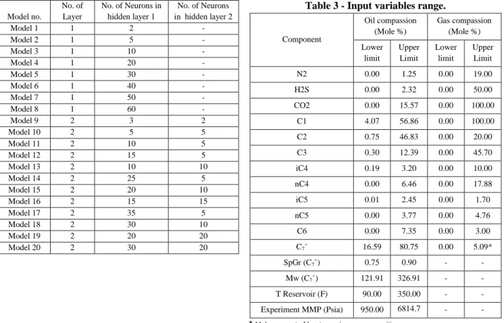
The structure of the neural network is constructed in a way that the difference between the predicted and observed (actual) values in the output vector is as small as possible. The most successful ANN architecture is the one that has the smallest prediction error on a data set for which it was not trainedor the one with the least difference between the correlation coefficients (R) of the training set and the testing set [17]. The total number of data utilized in this work is 128. In this study various neural network architectures were investigated in order to obtain desired models for predicting MMP as a function of selected input variables. Different models on the number of hidden layers as well as the number of neurons in each hidden layer were also analyzed (table 2).
The first and second hidden layers have TANSIG neurons. TANSIG is the “hyperbolic tangent sigmoid transfer function”. It calculates the output of a layer from its net input. The hidden layers have weights coming from the input. Each subsequent layer has a weight coming from the previous layer. Both layers have biases. The last layer is the network output.
Since the neural networks use neurons that can be trained, the universality of the model depends on the number and range of data. As the number and range of data increases, the universality of the model shall also increase. Table 3 shows the range on input data wider than other models.
Table 2 - Different neural networks models.
Model no.
No. of Layer
No. of Neurons in hidden layer 1
No. of Neurons in hidden layer 2
Model 1 1 2 -
Model 2 1 5 -
Model 3 1 10 -
Model 4 1 20 -
Model 5 1 30 -
Model 6 1 40 -
Model 7 1 50 -
Model 8 1 60 -
Model 9 2 3 2
Model 10 2 5 5
Model 11 2 10 5
Model 12 2 15 5
Model 13 2 10 10
Model 14 2 25 5
Model 15 2 20 10
Model 16 2 15 15
Model 17 2 35 5
Model 18 2 30 10
Model 19 2 20 20
Model 20 2 30 20
This study concerns data collected from Glaso [16], Kuo [30], Firoozabadi [38], Metcalfe [5], Rathmell [32], Alston [15], Sebastian [22], Pedrod [6], Emera [23], slim-tube experiment on Iranian oil reservoir α& β [28] that it includes 128 oil and gas samples.
The following procedures were used after calculating necessary parameters for network training: 1) Normalizing the inputs and targets
2) Creating the network
3) Dividing up samples for testing 4) Training the network
5) Simulating the network 6) Reversing normalized outputs 7) Plot regression
Table 3 - Input variables range.
Component Oil compassion (Mole %) Gas compassion (Mole %) Lower limit Upper Limit Lower limit Upper Limit
N2 0.00 1.25 0.00 19.00
H2S 0.00 2.32 0.00 50.00
CO2 0.00 15.57 0.00 100.00
C1 4.07 56.86 0.00 100.00
C2 0.75 46.83 0.00 20.00
C3 0.30 12.39 0.00 45.70
iC4 0.19 3.20 0.00 10.00
nC4 0.00 6.46 0.00 17.88
iC5 0.01 2.45 0.00 1.70
nC5 0.00 3.77 0.00 4.76
C6 0.00 7.35 0.00 3.00
C7+ 16.59 80.75 0.00 5.09*
SpGr (C7+) 0.75 0.90 - -
Mw (C7+) 121.91 326.91 - -
T Reservoir (F) 90.00 350.00 - -
Experiment MMP (Psia) 950.00 6814.7 - -
5. Results and discussion
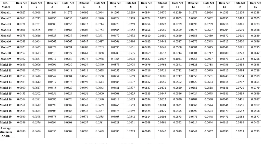
Initially, to investigate the ability of the developed gas–oil MMP model and also in order to avoid over-training, about 20 percent of the input-output data was randomly selected for the network testing and the rest was selected for network training and validation. After utilizing the program, a minimum average absolute relative error (AARE) for different models and data sets were gained (table 4).
Data set 4 has lowest minimum AARE among all other data sets. Minimum AARE is 0.0609 for this data set. Data set 4 was used to generate weight fraction mixing rules and Twu correlation to estimate critical temperature C7+.
Also actual critical temperatures were used for C2 and H2S components. To determine best neural network model
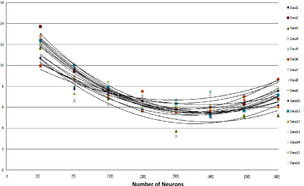
Fig. 1. Minimum average absolute relative error (AARE) versus different single hidden layer neural network.
Ab
so
lu
te Re
la
tive
Er
ror
(
%)
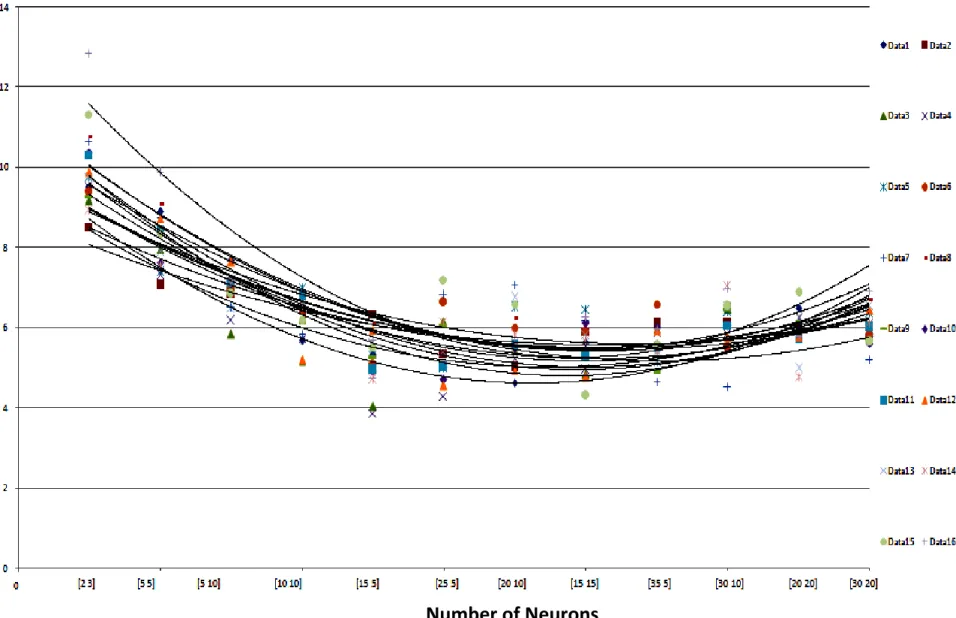
Fig. 2. Minimum average absolute relative error (AARE) versus different double hidden layers neural network.
Abs
o
lu
te Re
la
tive
Er
ror
(
%)
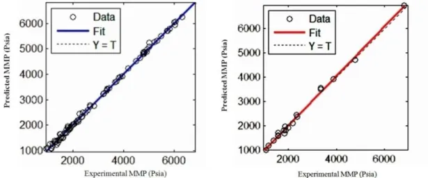
Typically, an application of back-propagation requires both a training set and a test set. Both the two sets contain input/output pattern pairs. While the training set is used to train the network, the test set is used to assess the performance of the network after the training is complete. To provide the best test of network performance, the test set should be different from the training set. The most successful ANN architecture is the one that has the smallest prediction error on a data set for which it was not trained. For Data Set 4 with model 5, 20 percent of data select for test set and training was run with 80 percent extant. The scatter plot in Fig. 3 presents comparison of the measured gas - oil MMP values with the new ANN model derived ones after training for Data Set 4. The results of the test data are shown in Fig.4
Fig. 3.The experimental versus ANN simulated gas-oil MMP (Train). Fig. 4.The experimental versus ANN simulated gas-oil MMP (Test).
Table 4 - Minimum average absolute relative error (AARE) for different models and data sets. NN. Model Data Set 1 Data Set 2 Data Set 3
Data Set 4 Data Set 5 Data Set 6 Data Set 7 Data Set 8 Data Set 9 Data Set 10 Data Set 11 Data Set 12 Data Set 13 Data Set 14 Data Set 15 Data Set 16
Model 1 0.0927 0.0968 0.1164 0.1272 0.0992 0.0994 0.1293 0.1299 0.0894 0.0970 0.1239 0.1279 0.1064 0.1035 0.1205 0.1288
Model 2 0.0863 0.0745 0.0796 0.0656 0.0793 0.0890 0.0729 0.0978 0.0724 0.0771 0.1003 0.0886 0.0682 0.0855 0.0889 0.0905
Model 3 0.0771 0.0761 0.0680 0.0656 0.0712 0.0714 0.0778 0.0769 0.0754 0.0727 0.0789 0.0698 0.0709 0.0716 0.0841 0.0773
Model 4 0.0601 0.0565 0.0613 0.0584 0.0703 0.0753 0.0585 0.0652 0.0656 0.0656 0.0569 0.0574 0.0627 0.0704 0.0599 0.0588
Model 5 0.0575 0.0616 0.0523 0.0237 0.0667 0.0591 0.0672 0.0632 0.0610 0.0550 0.0629 0.0558 0.0489 0.0572 0.0610 0.0639
Model 6 0.0541 0.0604 0.0562 0.0565 0.0745 0.0617 0.0568 0.0496 0.0625 0.0542 0.0517 0.0576 0.0543 0.0712 0.0620 0.0656
Model 7 0.0623 0.0635 0.0372 0.0591 0.0805 0.0703 0.0596 0.0661 0.0496 0.0641 0.0568 0.0681 0.0675 0.0649 0.0621 0.0715
Model 8 0.0557 0.0673 0.0518 0.0527 0.0761 0.0868 0.0780 0.0595 0.0669 0.0617 0.0714 0.0504 0.0747 0.0680 0.0778 0.0642
Model 9 0.0952 0.0851 0.0917 0.0950 0.0977 0.0938 0.1065 0.1078 0.0827 0.0837 0.1031 0.0958 0.0977 0.0873 0.1132 0.1256
Model 10 0.0689 0.0606 0.0796 0.0730 0.0639 0.0840 0.0875 0.0908 0.0676 0.0762 0.0541 0.0823 0.0788 0.0756 0.0836 0.0858
Model 11 0.0769 0.0704 0.0584 0.0618 0.0711 0.0638 0.0552 0.0679 0.0716 0.0711 0.0712 0.0525 0.0649 0.0715 0.0684 0.0718
Model 12 0.0558 0.0616 0.0647 0.0584 0.0640 0.0550 0.0454 0.0659 0.0657 0.0605 0.0717 0.0655 0.0551 0.0743 0.0654 0.0599
Model 13 0.0583 0.0642 0.0517 0.0573 0.0697 0.0643 0.0685 0.0697 0.0612 0.0655 0.0502 0.0420 0.0663 0.0614 0.0717 0.0651
Model 14 0.0509 0.0617 0.0615 0.0529 0.0499 0.0663 0.0681 0.0597 0.0637 0.0371 0.0620 0.0655 0.0538 0.0646 0.0720 0.0779
Model 15 0.0433 0.0502 0.0556 0.0524 0.0651 0.0600 0.0708 0.0625 0.0525 0.0547 0.0556 0.0424 0.0675 0.0581 0.0659 0.0659
Model 16 0.0564 0.0591 0.0585 0.0370 0.0646 0.0590 0.0617 0.0673 0.0534 0.0612 0.0630 0.0407 0.0580 0.0646 0.0431 0.0617
Model 17 0.0561 0.0612 0.0598 0.0587 0.0541 0.0659 0.0466 0.0553 0.0490 0.0604 0.0631 0.0563 0.0524 0.0641 0.0556 0.0767
Model 18 0.0534 0.0634 0.0503 0.0386 0.0533 0.0567 0.0476 0.0689 0.0525 0.0475 0.0495 0.0595 0.0564 0.0579 0.0552 0.0568
Model 19 0.0569 0.0598 0.0575 0.0629 0.0571 0.0585 0.0608 0.0542 0.0614 0.0593 0.0573 0.0476 0.0448 0.0471 0.0588 0.0577
Model 20 0.0549 0.0576 0.0594 0.0608 0.0637 0.0581 0.0521 0.0671 0.0568 0.0561 0.0552 0.0614 0.0644 0.0613 0.0566 0.0403
Average Minimum
AARE
0.0636 0.0656 0.0636 0.0609 0.0696 0.0699 0.0685 0.0723 0.0640 0.0640 0.0679 0.0644 0.0657 0.0690 0.0713 0.0733
Table 5 - Minimum AARE different models and data sets.
NN. Model Data Set 1 Data Set 2 Data Set 3
Data Set 4 Data Set 5 Data Set 6 Data Set 7 Data Set 8 Data Set 9 Data Set 10 Data Set 11 Data Set 12 Data Set 13 Data Set 14 Data Set 15 Data Set 16 Model
No. 15 15 7 5 14 13 13 6 17 14 18 16 19 19 16 20
Minimum
Table 6- Correlation coefficient and the error resulted for experimental MMPs and ANN predicted values.
Parameter AARE correlation coefficient
Training set 0.0237 0.999
Testing set 0.0325 0.998
More models present prediction of gas- oil MMP by researches that are used for pure CO2 or impure CO2. Several models are applied for determination of minimum miscibility pressure of the light hydrocarbon and flue gas. While U-ANN has more universality in comparison with the other models, it can predict minimum miscibility pressure for all types of gas in a wider range of input variable. This model is also accurate and has less error. In order to predict impure CO2 MMP, knowing the pure CO2 MMP value in all of previous models is required, while the new model directly predicts impure CO2 MMP with the effective parameters. Table 7 shows that the average relative error (ARE), average absolute relative error (AARE) and the standard deviation of error for the new proposed model are respectively 0.65 %, 2.37 %, and 3.03 % for 128 data. It should also be noted that Shokir models used 65 data in their model.
Table 7- Comparison of the gas–oil MMP obtained from the new U-ANN based model to the calculated gas– oil MMP from different literature models
UANN Shokir (2007) Shokir (2007) Emera and Sarma (2005) Emera and Sarma (2004) Dong (1999) Eakin and Mitch (1988) Alston et al. (1985) Alston et al. (1985) Glaso (1985) Sebasti an et al. (1985) Kovari k (1985)
ARE (%) 0.65 0.14 0.25 −0.62 0.65 2.28 63.11 −5.05 −5.37 −0.85 1.37 −23.43
AARE (%) 2.37 3.30 2.55 5.72 4.05 10.19 70.40 6.64 7.54 9.33 5.93 39.48
Standard
deviation (%) 3.03 4.67 3.11 7.15 4.25 15.17 46.83 7.51 7.26 7.18 7.55 51.69
Correlation
coefficient 0.999 0.998 0.998 0.970 0.993 0.910 0.50 0.960 0.967 0.970 0.950 0.830
No. Data 128 67 30 61 20 45 52 38 30 46 60 38
Pure CO2
Impure CO2
Hydrocarbon
and flue gas
Ultimately, to check and confirm the precision of the new U-ANN model, MMPs were calculated for 20 systems not used in building the model for CO2 and natural gas displacements of crude oils. The new model effectively predicted
the experimental gas–oil MMP, with a high precision, for existence of different non-CO2 components up to
70-mole%, and up to 45.7 mole% of C1 in the injected natural gas stream (as shown in Tables 8). From Tables 8, the
new model gives the precise prediction of the experimental gas–oil MMP for all the tested systems with the lowest average relative error and average absolute relative error among all tested gas–oil MMP correlations.
Table 8 - Comparison of gas–oil MMP approximated from the new U-ANN model to the experimental MMP and to the calculated MMP from different conventional correlations.
UANN Shokir (2007) Emera and Sarma (2004)
ARE (%) 0.16 0.19 0.05
AARE (%) 3.75 4.47 6.69
Standard deviation (%) 4.31 6.00 9.00
6. Conclusion
An attempt was made in this study to investigate the application of a neural networks concept for prediction of MMP in a gas injection process. The interrelations of MMP with different compositions of driving gas and reservoir temperature, molecular weight of C7+ oil fraction and different compositions of reservoir oil have been analyzed, all
were generated with deferent mixing rules as well as with C7+ critical property estimating correlations. Various
neural networks architectures were investigated to obtain desired models for predicting MMP as a function of selected input variables. Different scenarios on the number of hidden layers and the number of neurons in each hidden layer were analyzed in order to obtain the best fit to the given data.
The model was successfully applied to pure CO2, impure CO2, flue gas and hydrocarbon gas streams. The
comparison between the prediction accuracies of the universal neural network and other methods indicated that the neural network approach was more accurate in predicting MMP. The result showed that the weight-fraction mixing rule with Twu correlation to estimating C7+ critical property provides better results than the other methods. The
model was tested with 20 different data which were not used in the network training. The testing results from the U-ANN model and empirical correlations showed that the proposed model can predict the MMP with better accuracy than other available correlations.
Thus, the results of this study suggest that the neural network model with mixing-rules methods is more reliable than other statistical methods for predicting MMP. Specially, under conditions with limited field information, the neural network approach can produce a higher accuracy than other estimating methods.
7. References
[1] Mansoori, G.A., Savidge, J.L., Predicting Retrograde Phenomena and Miscibility Using Equation of State, SPE
Annual Technical Conference and Exhibition, 8-11 October, San Antonio, Texas, 1989.
[2] Wang, Y., Orr, F.M., Calculation of minimum miscibility pressure, Journal of Petroleum Science and
Engineering, Volume 73, Issues 3–4, September 2010, pp. 267-271
[3] Nasrifar, Kh., Mosfeghian, M., Journal of Petroleum Science and Engineering, Volume 42, Issues 2–4, April
2004, Pages 223-234
[4] Shokir, E.M. Eissa, M. CO2–oil minimum miscibility pressure model for impure and pure CO2 streams, Journal
of Petroleum Science and Engineering, Vol.58, No.1, 173-185. 2007
[5] Yellig, W.F. Metcalfe, R.S. Determination and prediction of CO2 minimum miscibility pressure, Journal of
Petroleum Technology, Vol.32, No.1, 160-168. 1980
[6] Pedrod, P. Prediction of minimum miscibility pressure in rich gas injection, M.Sc. Thesis Tehran University,
Tehran, 1995
[7] Christiansen, L. M. Haines, H.K. (1984) ‘Rapid Measurement of Minimum Miscibility Pressure with the Rising-Bubble Apparatus’ SPE Reservoir Engineering, Vol.2, No.4, 523-527.
[8] D. Zhou, F.M. Orr Jr., SPE J. 28 (1988) 19–25.
[9] Harmon, R.A., Grigg, R.B., Vapor-Density Measurement for Estimating Minimum Miscibility Pressure, SPE
Reserv Eng J, Volume 3, Number 4,p.p 1215–1220, 1988
[10] Orr, F.M. Jensen, C.M. (1984) ’Interpretation of Pressure-Composition Phase Diagrams for CO2/Crude-Oil Systems’, SPE Journal, 24 Vol.5, pp. 485-497.
[11Rao, D.N., Lee, J.I., Journal of Petroleum Science and Engineering, Vol. 35, Issues 3–4, August 2002, pp.
247-262.
[12] Cronquist, C. Carbon Dioxide Dynamic Displacement with Light Oils Reservoir, Fourth Annual U.S. DOE
Symposium, Tulsa, USA, 18-23. 1978
[13] Lee, J.I. ‘Effectiveness of carbon dioxide displacement under miscible and immiscible conditions’ Research
Report RR-40, Petroleum Recovery Institute, Calgary, Alberta. 1979
[14] Holm, L.W. Josendal, V.A. ‘Mechanisms of Oil Displacement by Carbon Dioxide’, Journal of Petroleum
Technology, Vol.26, No.12, 1427-1438. 1974
[15] Alston, R.B. Kokolis, G.P. and James, C.F. CO2 minimum miscibility pressure: a correlation for impure CO2
[16] Glaso, O. ’Generalized minimum miscibility pressure correlation’, SPE Journal, Vol.25, No.6, 927-934. 1985
[17] Dong, M. Huang, S. Srivastava, R., Effect of Solution Gas in Oil on CO2 Minimum Miscibility Pressure,
Annual Technical Meeting, Jun 14 - 18, Calgary, Alberta, Canada. 1999
[18] Emera, M.K. and Sarma, H.K. ‘A Reliable Correlation To Predict the Change in Minimum Miscibility Pressure When CO2 Is Diluted With Other Gases‘, SPE Reservoir Evaluation & Engineering, Vol.9, No.4, 366-373. 2006
[19] Kovarik, F.S., A minimum miscibility pressure study using impure CO2 and west Texas oil system, SPE
Production Technology Symposium, 11-12 November, Lubbock, Texas. 1985.
[20] Sebastian, H.M., Lawrence, D.D., Nitrogen minimum miscibility pressure’, SPE/DOE Enhanced Oil Recovery
Symposium, 22-24 April, Tulsa, Oklahoma. 1992.
[21] Eakin, B.E., Mitch, F.J., Measurement and Correlation of Miscibility Pressures of Reservoir Oils, SPE Annual
Technical Conference and Exhibition, 2-5 October, Houston, Texas, 1988
[22] Dong, M. Huang, S. Srivastava, R., Effect of Solution Gas in Oil on CO2 Minimum Miscibility Pressure,
Annual Technical Meeting, Jun 14 - 18, Calgary, Alberta, Canada. 1999
[23] Emera, M. K., Sarma, H. K., Use of Genetic Algorithm to Predict Minimum Miscibility Pressure (MMP)
between Flue Gases and Oil in Design of Flue Gas Injection Project, SPE Middle East Oil and Gas Show and
Conference, Mar 12 - 15, , Kingdom of Bahrain, 2005
[24] Johnson, J.P., Pollin, J.S., MEASUREMENT AND CORRELATION OF CO2 MISCIBILITY PRESSURES,
SPE/DOE Enhanced Oil Recovery Symposium, 5-8 April, Tulsa, Oklahoma. 1981.
[25] Orr Jr., F.M. and Silva, M.K. Effect of Oil Composition on Minimum Miscibility Pressure-Part 2, SPE
Reservoir Engineering, Vol.2, No.4, pp.479-491, 1987.
[26] Enick, R.M. Holder, G.D. Morsi, B.I. ‘A thermodynamic correlation for the minimum miscibility pressure in CO2 flooding of petroleum reservoir’ SPE Reservoir Engineering, Vol.3, No.1, 81-92. 1988
[27] Yuan, H. Johns, R.T. Egwuenu, A.M. Dindoruk, B. ‘Improves MMP correlation for CO2 floods using analytical gas flooding’, SPE Reservoir Evaluation & Engineering, Vol.8, No.5, 418-425. 2004
[28] Slim-tube report on Iranian oil reservoir α& β, NIOC_R&D, 2007
[29] Haykin, S (2004) ‘Neural Networks: A Comprehensive Foundation’ (2nd Ed. Prentice Hall Publishing,, New
Jersey.
[30] Kou, L., Prediction of miscibility for enriched gas drive process, SPE Journal, Vol.34, No.2, 1985
[31] Poling, B.E., Prausnitz, J. M., The Properties of Gases and Liquids, McGraw-Hill, New York, 2004.
[32] Rathmell, J.J., Stalkup, F.I., Hassinger, R.C., A Laboratory Investigation of Miscible Displacement by Carbon
Dioxide, Fall Meeting of the Society of Petroleum Engineers of AIME, 3-6 October, New Orleans, Louisiana, 1971.
[33] Metcalfe, R.S., Yarborough, L., The Effect of Phase Equlilbria on the CO2 Displacement Mechanism, SPE J.
Vol. 9, No.4, pp. 242–252. 1979
[34] RUTHERFORD, W.M., Miscibility Relationships in the Displacement of Oil By Light Hydrocarbons, SPE J.,
Vol. 2, No.4, pp. 340–346, 1962
[35] Jacobson, H.A, J. Canada. Pet. Tech. 56, 1972.
[36] Ahmed, T. ‘Hydrocarbon Phase Behavior’, Gulf Publishing Company, Houston. 1989
[37] Boozarjomehry, R.B; Abdolahi, F.; Moosavian, M.A., Characterization of Basic Properties of Pure substances
and Petroleum Fractions by Neural Network, Fluid Phase Equlilbria, Vol. 231, No.2, pp.188-196, 2005.
[38] Firoozabadi, A., Aziz, k., Analysis and correlation of nitrogen and lean gas miscibility pressure, SPE Reservoir