Solving Engineering Optimization Problems with the Simple Constrained
Particle Swarm Optimizer
Leticia C. Cagnina and Susana C. Esquivel
LIDIC, Universidad Nacional de San Luis, San Luis, Argentina E-mail: [email protected]
Carlos A. Coello Coello
CINVESTAV-IPN, Mexico D. F., Mexico
Keywords:constrained optimization, engineering problems, particle swarm optimization
Received:July 7, 2008
This paper introduces a particle swarm optimization algorithm to solve constrained engineering optimiza-tion problems. The proposed approach uses a relatively simple method to handle constraints and a different mechanism to update the velocity and position of each particle. The algorithm is validated using four stan-dard engineering design problems reported in the specialized literature and it is compared with respect to algorithms representative of the state-of-the-art in the area. Our results indicate that the proposed scheme is a promising alternative to solve this sort of problems because it obtains good results with a low number of objective functions evaluations.
Povzetek: ˇClanek uvaja za reševanje inženirskih optimizacijskih problemov z omejitvami algoritem za optimizacijo z roji.
1 Introduction
Engineering design optimization problems are normally adopted in the specialized literature to show the ef-fectiveness of new constrained optimization algorithms. These nonlinear engineering problems have been inves-tigated by many researchers that used different methods to solve them: Branch and Bound using SQP [24], Re-cursive Quadratic Programming [9], Sequential Lineariza-tion Algorithm [20], Integer-discrete-continuous Nonlin-ear Programming [11], NonlinNonlin-ear Mixed-discrete Pro-gramming [19], Simulated Annealing [27], Genetic Algo-rithms [26], Evolutionary Programming [8] and, Evolution Strategies [25] among many others. These types of prob-lems normally have mixed (e.g., continuous and discrete) design variables, nonlinear objective functions and nonlin-ear constraints, some of which may be active at the global optimum. Constraints are very important in engineering design problems, since they are normally imposed on the statement of the problems and sometimes are very hard to satisfy, which makes the search difficult and inefficient.
Particle Swarm Optimization (PSO) is a relatively re-cent bio-inspired metaheuristic, which has been found to be highly competitive in a wide variety of optimization lems. However, its use in engineering optimization prob-lems and in constrained optimization probprob-lems, in general, has not been as common as in other areas (e.g., for adjust-ing weights in a neural network). The approach described in this paper contains a constraint-handling technique as well as a mechanism to update the velocity and position of
the particles, which is different from the one adopted by the original PSO.
This paper is organized as follows. Section 2 briefly dis-cusses the previous related work. Section 3 describes in detail our proposed approach. Section 4 presents the ex-perimental setup adopted and provides an analysis of the results obtained from our empirical study. Our conclusions and some possible paths for future research are provided in Section 5.
2 Literature review
Guo et al. presented a hybrid swarm intelligent algorithm with an improvement in global search reliability. They tested the algorithm with two of the problems adopted here (E02 and E04). Despite they claim that their algorithm is superior for finding the best solutions (in terms of qual-ity and robustness), the solution that they found for E02 is greater than its best known value and for E04 the results ob-tained are not comparable to ours, because they used more constraints in the definition of that problem [13].
E01, 19,154 for E02 and 12,630 for E03 [1].
Mahdavi et al. developed an improved harmony search algorithm with a novel method for generating new solutions that enhances the accuracy and the convergence rate of the harmony search. They used three of the problems adopted here (E01, E03 and E04) to validate their approach, per-forming 300,000, 200,000 and 50,000 evaluations, respec-tively. For E01 and E02, the best values reported are not the best known values because the ranges of some variables in E01 are different from those of the original description of the problem (x4 is out of range), which makes such
so-lution infeasible under the description adopted here. The value reported by them for E04 is very close to the best value known [21].
Bernardino et al. hybridized a genetic algorithm embed-ding an artificial immune system into its search engine, in order to help moving the population into the feasible re-gion. The algorithm was used to solve four of the test problems adopted here (E01, E02, E03 and E04), using 320,000, 80,000, 36,000 and 36,000 evaluations of the ob-jective functions, respectively. The best values found for E01, E02 and E04 are close to the best known. For E03 the value reported is better than the best known, because one of the decision variables is out of range (x5). The values in
general, are good, although the number of evaluations re-quired to obtain them is higher than those rere-quired by other algorithms [4].
Hernandez Aguirre et al. proposed a PSO algorithm with two new perturbation operators aimed to prevent prema-ture convergence, as well as a new neighborhood struc-ture. They used an external file to store some particles and, in that way, extend their life after the adjustment of the tolerance of the constraints. The authors reference three algorithms which obtained good results for the prob-lems adopted in their study: two PSO-based algorithms and a Differential Evolution (DE) algorithm. One of the PSO-based approaches compared [16] used three of the problems adopted here (E01, E02 and E04), performing 200,000 objective function evaluations. The other PSO-based approach compared [14] was tested with the same set of problems and the best known values were reached for E02 and E04 after 30,000 objective function evaluations. The DE algorithm [22] reported good results with 30,000 evaluations for the four problems. This same number of evaluations was performed by the algorithm proposed by Hernandez et al. and their results are the best reported until now for the aforementioned problems [15].
For that reason, we used these last two algorithms to compare the performance of our proposed approach. The DE algorithm [22] will be referenced as “Mezura” and, the PSO by [15] as “COPSO”.
3 Our proposed approach: SiC-PSO
The particles in our proposed approach (called Simple
ConstrainedParticleSwarmOptimizer, or SiC-PSO), are
n-dimensional values (continuous, discrete or a combina-tion of both) vectors, wherenrefers to the number of de-cision variables of the problem to be solved. Our approach adopts one of the most simple constraint-handling meth-ods currently available. Particles are compared by pairs: 1) if the two particles are feasible, we choose the one with a better fitness function value; 2) if the two particles are infeasible, we choose the particle with the lower infeasi-bility degree; 3) if one particle is feasible and the other is infeasible, we choose the feasible one. This strategy is used when thepbest,gbestandlbestparticles are chosen. When an individual is found infeasible, the amount of vi-olation (this value is normalized with respect to the largest violation stored so far) is added. So, each particle saves its infeasibility degree reached until that moment.
As in the basic PSO [10], our proposed algorithm records the best position found so far for each particle (pbestvalue) and, the best position reached by any particle into the swarm (gbestvalue). In other words, we adopt the gbest
model. But in previous works, we found that the gbest
model tends to converge to a local optimum very often [7]. Motivated by this, we proposed a formula to update the ve-locity, using a combination of both thegbestand thelbest
models [5]. Such a formula (Eq. 1) is adopted here as well. Thelbestmodel is implemented using a ring topology [17] to calculate the neighborhoods of each particle. For a size of neighborhood of three particles and a swarm of six parti-cles (1,2,3,4,5,6), the neighborhoods considered are the fol-lowing: (1,2,3), (2,3,4), (3,4,5), (4,5,6), (5,6,1) and (6,1,2). The formula for updating particles is the same that in the basic PSO and it is shown in Eq. 2.
vid = w(vid+c1r1(pbid−pid)
+c2r2(plid−pid) (1)
+c3r3(pgd−pid))
pid =pid+vid (2)
wherevid is the velocity of the particleiat the dimension d,wis the inertia factor [10] whose goal is to balance the global exploration and the local exploitation,c1is the
per-sonal learning factor, andc2,c3are the social learning
fac-tors, r1, r2 andr3 are three random numbers within the
range [0..1], pbid is the best position reached by the par-ticlei,plid is the best position reached by any particle in the neighborhood of particleiand,pgdis the best position reached by any particle in the swarm. Finally, pid is the value of the particleiat the dimensiond.
The standard deviation is the difference between these two values. We adapted that formula adding the global best (gbest) to the best position of the particle and the best in its neighborhood. We also changed the way in which the stan-dard deviation is determined. We use the pbestand, the
gbestinstead of thelbestas was proposed by Kennedy. We determined those changes after several empirical tests with different Gaussian random generator parameters. Thus, the position is updated using the following equation:
pi=N µ
pi+pli+pg
3 ,|pi−pg|
(3)
wherepi,pli andpg are defined as before and, N is the value returned by the Gaussian random generator. SiC-PSO used Eq. 3 and Eq. 2 for the updating of positions of the particles. We considered a high probability for se-lecting Eq. 3 (0.925) over Eq. 2. We chose that probability after conducting numerous experiments.
4 Parameter settings and analysis of
results
A set of 4 engineering design optimization problems was chosen to evaluate the performance of our proposed algo-rithm. A detailed description of the test problems may be consulted in the appendix at the end of this paper. We performed 30 independent runs per problem, with a total of 24,000 objective function evaluations per run. We also tested the algorithm with 27,000 and 30,000 evaluations of the objective function, but no performance improvements were noticed in such cases. Our algorithm used the follow-ing parameters: swarm size = 8 particles, neighborhood size = 3, inertia factor w = 0.8, personal learning factor and social learning factors forc1,c2andc3were set to 1.8.
These parameter settings were empirically derived after nu-merous previous experiments.
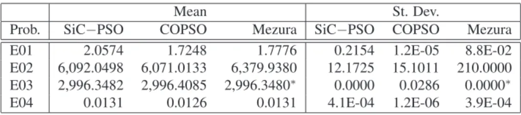
Our results were compared with respect to the best re-sults reported in the specialized literature. Those values were obtained by Hernandez Aguirre et al. [15] and Mezura et al. [22]. We reference those results into the tables shown next as “COPSO” and “Mezura”, respectively. It is impor-tant remark that COPSO and Mezura algorithms reached the best values after 30,000 fitness function evaluations, which is a larger value than that required by our algorithm. The best values are shown in Table 1 and, the mean and standard deviations over the 30 runs are shown in Table 2.
The three algorithms reached the best known values for E01. For E02, SiC-PSO and COPSO reached the best known, but Mezura reported a value with a precision of only 4 digits after the decimal point, and the exact value reached by them is not reported. For E03, SiC-PSO reached the best value, COPSO reached a value slightly worse than ours, and Mezura reached an infeasible value. SiC-PSO and COSiC-PSO reached the best value for E04, although Mezura reported a value that is worse than the best known. In general, COPSO obtained the best mean values, except
for E03 for which best mean was found by our algorithm. The lower standard deviation values for E01 and E04 was obtained by COPSO; for E02 and E03, our SiC-PSO found the minimum values.
Tables 3, 4, 5 and 6 show the solution vectors of the best solution reached by SiC-PSO as well as the values of the constraints, for each of the problems tested.
Best Solution
x1 0.205729
x2 3.470488
x3 9.036624
x4 0.205729
g1(~x) -1.819E-12
g2(~x) -0.003721
g3(~x) 0.000000
g4(~x) -3.432983
g5(~x) -0.080729
g6(~x) -0.235540
g7(~x) 0.000000
f(~x) 1.724852
Table 3: SiC-PSO Solution vector for E01 (welded beam).
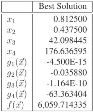
Best Solution
x1 0.812500
x2 0.437500
x3 42.098445
x4 176.636595
g1(~x) -4.500E-15
g2(~x) -0.035880
g3(~x) -1.164E-10
g4(~x) -63.363404
f(~x) 6,059.714335
Table 4: SiC-PSO Solution vector for E02 (pressure ves-sel).
5 Conclusions and Future Work
Prob. Optimal SiC−PSO COPSO Mezura
E01 1.724852 1.724852 1.724852 1.724852
E02 6,059.714335 6,059.714335 6,059.714335 6,059.7143 E03 NA 2,996.348165 2,996.372448 2,996.348094∗
E04 0.012665 0.012665 0.012665 0.012689
∗Infeasible solution. NA Not avaliable.
Table 1: Best results obtained by SiC-PSO, COPSO and Mezura.
Mean St. Dev.
Prob. SiC−PSO COPSO Mezura SiC−PSO COPSO Mezura
E01 2.0574 1.7248 1.7776 0.2154 1.2E-05 8.8E-02
E02 6,092.0498 6,071.0133 6,379.9380 12.1725 15.1011 210.0000 E03 2,996.3482 2,996.4085 2,996.3480∗ 0.0000 0.0286 0.0000∗
E04 0.0131 0.0126 0.0131 4.1E-04 1.2E-06 3.9E-04
∗Infeasible solution.
Table 2: Means and Standard Deviations for the results obtained.
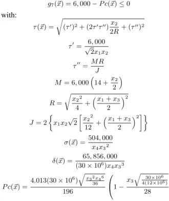
Best Solution
x1 3.500000
x2 0.700000
x3 17
x4 7.300000
x5 7.800000
x6 3.350214
x7 5.286683
g1(~x) -0.073915
g2(~x) -0.197998
g3(~x) -0.499172
g4(~x) -0.901471
g5(~x) 0.000000
g6(~x) -5.000E-16
g7(~x) -0.702500
g8(~x) -1.000E-16
g9(~x) -0.583333
g10(~x) -0.051325
g11(~x) -0.010852
f(~x) 2,996.348165
Table 5: SiC-PSO Solution vector for E03 (speed reducer).
other algorithms. Thus, we consider our approach to be a viable choice for solving constrained engineering optimiza-tion problems, due to its simplicity, speed and reliability. As part of our future work, we are interested in exploring other PSO models and in performing a more detailed statis-tical analysis of the performance of our proposed approach.
Appendix: Engineering problems
Formulating of the engineering design problems used to test the algorithm proposed.
Best Solution
x1 0.051583
x2 0.354190
x3 11.438675
g1(~x) -2.000E-16
g2(~x) -1.000E-16
g3(~x) -4.048765
g4(~x) -0.729483 f(~x) 0.012665
Table 6: SiC-PSO Solution vector for E04 (ten-sion/compression spring).
E01: Welded beam design optimization
problem
The problem is to design a welded beam for minimum cost, subject to some constraints [23]. Figure 1 shows the welded beam structure which consists of a beam A and the weld required to hold it to member B. The objective is to find the minimum fabrication cost, considerating four design variables: x1, x2, x3,x4 and constraints of shear
stressτ, bending stress in the beamσ, buckling load on the barPc, and end deflection on the beamδ. The optimization model is summarized in the next equation:
Minimize:
f(~x) = 1.10471x12x2+ 0.04811x3x4(14.0 +x2)
subject to:
g1(~x) =τ(~x)−13,600≤0
g2(~x) =σ(~x)−30,000≤0
g3(~x) =x1−x4≤0
g4(~x) = 0.10471(x12) + 0.04811x3x4(14 +x2)−5.0≤0
g5(~x) = 0.125−x1≤0
g7(~x) = 6,000−P c(~x)≤0
with:
τ(~x) = r
(τ0)2+ (2τ0τ00)x2
2R+ (τ00)2
τ0=√6,000
2x1x2
τ00= M R
J
M= 6,000 ³
14 +x2 2 ´
R= r
x22
4 +
³x
1+x3 2
´2
J= 2 ½
x1x2
√
2 ·
x22
12 +
³x
1+x3 2
´2¸¾
σ(~x) = 504,000
x4x32
δ(~x) = 65,856,000 (30×106)x
4x33
P c(~x) =4.013(30×10 6)
q
x32x46 36 196
1−x3 q
30×106 4(12×106)
28
with0.1≤x1, x4≤2.0, and0.1≤x2, x3≤10.0.
Best solution:
x∗= (0.205730,3.470489,9.036624,0.205729)
wheref(x∗) = 1.724852.
Figure 1: Weldem Beam.
E02: Pressure Vessel design optimization
problem
A compressed air storage tank with a working pressure of 3,000 psi and a minimum volume of 750 ft3. A cylindrical
vessel is capped at both ends by hemispherical heads (see Fig. 2). Using rolled steel plate, the shell is made in two halves that are joined by teo longitudinal welds to form a cylinder. The objective is minimize the total cost, including the cost of the materials forming the welding [24]. The de-sign variables are: thicknessx1, thickness of the headx2,
the inner radiusx3, and the length of the cylindrical section
of the vesselx4. The variablesx1andx2are discrete
val-ues which are integer multiples of 0.0625 inch. Then, the formal statement is:
Minimize:
f(~x) = 0.6224x1x3x4+ 1.7781x2x32+ 3.1661x12x4 + 19.84x12x3
subject to:
g1(~x) =−x1+ 0.0193x3≤0
g2(~x) =−x2+ 0.00954x3≤0
g3(~x) =−πx32x42−4 3πx3
3
+ 1,296,000≤0
g4(~x) =x4−240≤0
with1×0.0625≤x1, x2≤99×0.0625,10.0≤x3, and
x4≤200.0.
Best solution:
x∗= (0.8125,0.4375,42.098446,176.636596)
wheref(x∗) = 6,059.714335.
Figure 2: Pressure Vessel.
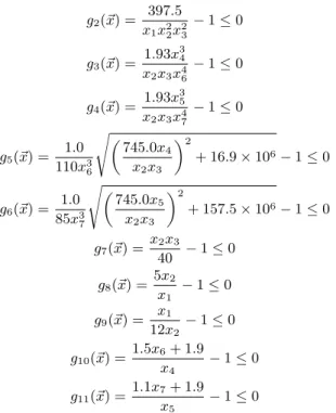
E03: Speed Reducer design optimization
problem
The design of the speed reducer [12] shown in Fig. 3, is considered with the face width x1, module of teeth x2,
number of teeth on pinion x3, length of the first shaft
between bearingsx4, length of the second shaft between
bearings x5, diameter of the first shaft x6, and diameter
of the first shaft x7 (all variables continuous except x3
that is integer). The weight of the speed reducer is to be minimized subject to constraints on bending stress of the gear teeth, surface stress, transverse deflections of the shafts and stresses in the shaft. The problem is:
Minimize:
f(~x) = 0.7854x1x22(3.3333x23+ 14.9334x3−43.0934)
−1.508x1(x26+x27) + 7.4777(x36+x37) + 0.7854(x4x26+x5x27)
subject to:
g1(~x) = 27
g2(~x) = 397.5
x1x22x23
−1≤0
g3(~x) = 1.93x 3 4
x2x3x46
−1≤0
g4(~x) = 1.93x 3 5
x2x3x47
−1≤0
g5(~x) = 1.0 110x3
6
sµ 745.0x4
x2x3
¶2
+ 16.9×10⁶−1≤0
g6(~x) = 1.0 85x3
7
sµ 745.0x5
x2x3
¶2
+ 157.5×10⁶−1≤0
g7(~x) = x2x3
40 −1≤0
g8(~x) =5x2
x1
−1≤0
g9(~x) = x1
12x2 −1≤0
g10(~x) = 1.5x6+ 1.9
x4 −1≤0
g11(~x) = 1.1x7+ 1.9
x5
−1≤0
with 2.6 ≤ x1 ≤ 3.6,0.7 ≤ x2 ≤ 0.8,17 ≤ x3 ≤
28,7.3 ≤x4 ≤8.3,7.8≤x5≤8.3,2.9≤x6≤3.9, and
5.0≤x7≤5.5.
Best solution:
x∗ = (3.500000,0.7,17,7.300000,7.800000,
3.350214,5.286683)
wheref(x∗) = 2,996.348165.
Figure 3:Speed Reducer.
5.1 E04: Tension/compression spring design
optimization problem
This problem [2] [3] minimizes the weight of a ten-sion/compression spring (Fig. 4), subject to constraints of minimum deflection, shear stress, surge frequency, and limits on outside diameter and on design variables. There are three design variables: the wire diameterx1, the mean
coil diameterx2, and the number of active coilsx3. The
mathematical formulation of this problem is:
Minimize:
f(~x) = (x3+ 2)x2x21
subject to:
g1(~x) = 1− x 3 2x3 7,178x4
1
≤0
g2(~x) = 4x 2 2−x1x2 12,566(x2x31)−x41
+ 1
5,108x2 1
−1≤0
g3(~x) = 1−140.45x1
x2
2x3 ≤0
g4(~x) = x2+x1
1.5 −1≤0
with 0.05 ≤ x1 ≤ 2.0,0.25 ≤ x2 ≤ 1.3, and
2.0≤x3≤15.0.
Best solution:
x∗= (0.051690,0.356750,11.287126)
wheref(x∗) = 0.012665.
Figure 4: Tension/Compression Spring.
Acknowledgment
The first and second author acknowledge support from the ANPCyT (National Agency to Promote Science and Tech-nology, PICT 2005 and Universidad Nacional de San Luis. The third author acknowledges support from CONACyT project no. 45683-Y.
References
[1] S. Akhtar, K. Tai and T. Ray. A Socio-behavioural Simulation Model for Engineering Design Optimiza-tion.Eng. Optimiz., 34(4):341–354, 2002.
[3] A. Belegundu. A Study of Mathematical Program-ming Methods for Structural Optimization. PhD the-sis, Department of Civil Environmental Engineering, University of Iowa, Iowa, 1982.
[4] H. Bernardino, H. Barbosa and A. Lemonge. A Hy-brid Genetic Algorithm for Constrained Optimization Problems in Mechanical Engineering. InProc. IEEE Congress on Evolutionary Computation (CEC 2007), Singapore, 2007, pages 646–653.
[5] L. Cagnina, S. Esquivel and C. Coello Coello. A Particle Swarm Optimizer for Constrained Numerical Optimization. InProc. 9th International Conference on Parallel Problem Solving from Nature (PPSN IX), Reykjavik, Iceland, 2006, pages 910–919.
[6] L. Cagnina, S. Esquivel and C. Coello Coello. A Bi-population PSO with a Shake-Mechanism for Solving Constrained Numerical Optimization. InProc. IEEE Congress on Evolutionary Computation (CEC2007), Singapore, 2007, pages 670–676.
[7] L. Cagnina, S. Esquivel and R. Gallard. Particle Swarm Optimization for Sequencing Problems: a Case Study. InProc. IEEE Congress on Evolutionary Computation (CEC 2004), Portland, Oregon, USA, 2004, pages 536–541.
[8] Y. Cao and Q. Wu. Mechanical Design Optimiza-tion by Mixed-variable EvoluOptimiza-tionary Programming. In1997 IEEE International Conference on Evolution-ary Computation, Indianapolis, Indiana, USA, 1997, pages 443–446.
[9] J. Cha and R. Mayne. Optimization with Discrete Variables via Recursive Quadratic Programming: part II.J. Mech. Transm.-T. ASME, 111(1):130–136, 1989.
[10] R. Eberhart and Y. Shi. A Modified Particle Swarm Optimizer. In Proc. IEEE International Conference on Evolutionary Computation, Anchorage, Alaska, USA, 1998, pages 69–73.
[11] J. Fu, R. Fenton and W. Cleghorn. A Mixed Integer-discrete-continuous Programming Method and its Applications to Engineering Design Optimization.
Eng. Optimiz., 17(4):263–280, 1991.
[12] J. Golinski. An Adaptive Optimization System Ap-plied to Machine Synthesis. Mech. Mach. Theory, 8(4):419 ˝U436, 1973.
[13] C. Guo, J. Hu, B. Ye and Y. Cao. Swarm Intelligence for Mixed-variable Design Optimization.J. Zheijiang University Science, 5(7):851–860, 1994.
[14] S. He, E. Prempain and Q. Wu. An Improved Particle Swarm Optimizer for Mechanical Design Optimiza-tion Problems.Eng. Optimiz., 36(5):585–605, 2004.
[15] A. Hernandez Aguirre, A. Muñoz Zavala, E. Villa Di-harce and S. Botello Rionda. COPSO: Constrained Optimization via PSO Algorithm. Technical report No. I-07-04/22-02-2007, Center for Research in Mathematics (CIMAT), 2007.
[16] X. Hu, R. Eberhart and Y. Shi. Engineering Opti-mization with Particle Swarm. InProc. IEEE Swarm Intelligence Symposium, Indianapolis, Indiana, USA, 2003, pages 53–57.
[17] J. Kennedy. Small World and Mega-Minds: Effects of Neighborhood Topologies on Particle Swarm Perfor-mance. InIEEE Congress on Evolutionary Computa-tion (CEC 1999), Washington, DC, USA, 1999, pages 1931–1938.
[18] J. Kennedy and R. Eberhart. Bores Bones Particle Swarm. In Proc. IEEE Swarm Intelligence Sympo-sium, Indianapolis, Indiana, USA, 2003, pages 80– 89.
[19] H. Li and T. Chou. A Global Approach of Nonlinear Mixed Discrete Programming in Design Optimiza-tion.Eng. Optimiz., 22(2):109–122, 1993.
[20] H. Loh and P. Papalambros. A Sequential Lineariza-tion Approach for Solving Mixed-discrete Nonlin-ear Design Optimization Problems.J. Mech. Des.-T. ASME, 113(3):325–334, 1991.
[21] M. Mahdavi, M. Fesanghary and E. Damangir. An Improved Harmony Search Algorithm for Solv-ing Optimization Problems. Appl. Math. Comput., 188(2):1567–1579, 2007.
[22] E. Mezura and C. Coello. Useful Infeasible Solutions in Engineering Optimization with Evolutionary Al-gorithms. Lect. Notes Comput. Sc., 3789:652–662, 2005.
[23] K. Ragsdell and D. Phillips. Optimal Design of a Class of Welded Structures using Geometric Pro-gramming.J. Eng. Ind., 98(3):1021–1025, 1976.
[24] E. Sandgren. Nonlinear Integer and Discrete Pro-gramming in Mechanical Design Optimization. J. Mech. Des.-T. ASME, 112(2):223–229, 1990.
[25] G. Thierauf and J. Cai. Evolution Strategies - Paral-lelization and Applications in Engineering Optimiza-tion. InParallel and Distributed Precessing for Com-putational Mechanics. B.H.V. Topping (ed.), Saxe-Coburg Publications, 2000, pages 329–349.